Heterodyne Near Field Speckles: from laser light to X-rays

ABSTRACT

A fascinating way of generating speckle patterns is by interfering the weak fields scattered by a disordered sample with the intense trans-illuminating beam. The resulting intensity fluctuations are known as Heterodyne Near Field Speckles. Thanks to the self-referencing layout, the intensity distribution allows direct assessment of the electric fields, thus preserving both amplitude and phase information. Originally observed with visible laser light, during the last years Heterodyne Near Field Speckles have been extended to partially coherent radiation and to X-ray beams. We give in this review a uniform argumentation of Heterodyne Near Field Speckles based on Fourier Optics, valid with both coherent and partially coherent illumination. Emphasis is given to the speckle size, a fundamental property of any speckle field and a basis for earlier and state-of-the-art development of the technique. We review the applications of Heterodyne Near Field Speckles in the fields of particle sizing, velocimetry, coherence measurements, X-ray wavefront sensing and X-ray phase-contrast imaging and tomography. Throughout the discussion, we also emphasize the common aspects shared with many different research areas, such as astronomical observations, holography and TEM imaging, thus evidencing the encompassing nature of the underlying physical principles.

Graphical abstract

KEYWORDS:

• Speckle and Moiré Pattern
• Fourier Optics
• Holography
• Coherence
• Synchrotron Radiation

PACS:

• 42.30.Ms
• 42.30.Kq
• 42.40.-i
• 42.25.Kb
• 41.60.Ap

1. Introduction

Within the realm of statistical optics, the granular noise-like intensity distributions observed when electromagnetic radiation interacts with objects that are rough on the scale of a wavelength are nowadays known as speckles. Speckles are ubiquitous whenever coherent radiation is used, the most common example being a laser beam reflected from a rough surface [1,2]. Indeed, the interest in speckle patterns experienced an incredible boost since the first lasers became available in the early 1960s. Nevertheless, earlier observations date back to the time of Newton [3]. Before the introduction of lasers, speckles have been primarily investigated in connection to scattering experiments from random media enlightened by poorly coherent sources such as candles [4–6]. Exceptionally, the speckle phenomenon has also been reproduced in famous paintings by artists looking at polychromatic light sources with the unaided eye [7,8].

Speckles arise due to the mutual interference among a number of randomly-phased scattered waves. Whether this superposition occurs coherently or incoherently strongly differentiates laser speckles from speckles in partially coherent light. Speckles in fully coherent light are described by the Van Cittert and Zernike theorem [1,2,9–11]. In free-space propagation conditions, it relates the autocorrelation function of laser speckle patterns, describing the average size and shape of speckles, to the Fourier transform of the source intensity distribution (objective speckles). In imaging geometry, the theorem still holds by replacing the light source with the entrance pupil of the optics (subjective speckles). On the other hand, polychromatic speckles have an elongated radial structure which ultimately results from the finite bandwidth of the light source, i.e. from the limited temporal coherence of the emitted radiation [1,12,13]. Partial spatial coherence basically reduces the speckle contrast and in some cases it results in an increased speckle size [1].

All the aforementioned cases are examples of so-called homodyne speckles arising from the mutual interference among the scattered waves only. The incident beam is either totally scattered or negligible with respect to the diffused light. Typically, speckles are observed in the far field of the sample or by imaging the scattering surface.

At the opposite case, a fascinating way of generating speckle patterns is by interfering the weak scattered fields with the strong trans-illuminating beam and by further observing the resulting intensity distribution close enough to the scattering sample. Such speckles are called Heterodyne (i.e. self-referencing) Near Field Speckles [14–16]. The self-referencing geometry and the near-field conditions allow direct measurements of the scattered field, thus preserving both amplitude and phase information. With coherent light, this provides direct access to the static and dynamic scattering information of the sample [14–24], as well as to velocimetry measurements [25–27]. Under partially coherent light, direct measurements of the spatial and temporal coherence properties of the illuminating beam are possible [28,29]. The fundamentals of Heterodyne Near Field Speckles are largely wavelength-independent, thus paving the way to analogous experiments with X-rays [30–40]. Furthermore, during the last years, X-ray Heterodyne Near Field Speckles have also been largely exploited for X-ray beam wavefront sensing [41–44], in-line at-wavelength metrology of X-ray optics [45–55], and X-ray phase-contrast imaging and tomography [56–83].

This paper provides an overview of the principles and the state-of-the-art of Heterodyne Near Field Speckles, guiding the reader through the historical development of the technique. The work is organized as follows. Starting with the case of visible laser light in Section 2, we deal with the origin of self-referencing speckles in Section 2.1. In Section 2.2 we introduce a formalism based on Fourier Optics [84] to describe their power spectrum and autocorrelation function. In Section 2.3 we focus on the peculiar Talbot oscillations appearing in the power spectrum, discussing their origin and the most common causes that make them vanish. We then give a review about earlier and recent results and applications with coherent radiation in Section 2.4. In Section 3 we extend the discussion and the mathematical framework to the case of partially coherent radiation. It represents the link with, and the background to, Section 4, where we show how self-referencing speckles naturally arise with X-rays. Sections 4.1, 4.2, 4.3 and 4.4 review the wide range of techniques developed in the last years at large-scale facilities such as synchrotrons and Free Electron Lasers (FELs). Finally, in Section 5 we show how the Fourier Optics approach, based on plane wave decomposition of the incident and the scattered fields, provides a unified description of Heterodyne Near Field Speckles common to all the applications and wavelength domains. Particular emphasis is given to the speckle size under various illumination conditions.

2. Heterodyne Near Field Speckles in coherent light

2.1. On the origin of heterodyne speckles

We start by considering a collimated laser beam with diameter $D$ and wavelength $\lambda$ impinging onto a water suspension of spherical particles with diameter $d$ (a colloidal suspension). Any other disordered ensemble of scattering centers would be just suitable, as for example membranes or a piece of sandpaper. However, colloidal suspensions play a central role in the development of Heterodyne Near Field Speckles, both from the historical and conceptual point of view. Furthermore, they offer several practical advantages over other systems, thus allowing a straightforward implementation of the technique. We refer the reader to the cited literature for further details.

Each particle scatters a weak spherical wave which interferes with the stronger transmitted beam. We will always consider the elastic scattering regime, where the incident beam and the scattered light have the same wavelength. The resulting intensity distribution is observed at a distance $z$ downstream the sample, as sketched in Figure 1. In case of a diverging illuminating wavefront from a point source at a distance $R$ from the sample, the same formalism can be applied by considering an effective propagation distance $z_{\mathrm{e}\mathrm{f}\mathrm{f}}=z(1+z/R)$ and a geometrical magnification $m=1+z/R$ at the observation plane (Fresnel scaling theorem [85]).

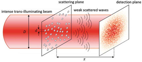
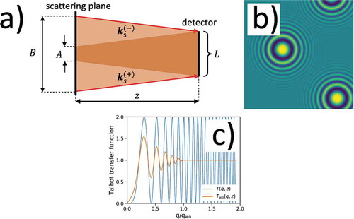
Figure 1. A sketch of the self-referencing (heterodyne) layout. The weak spherical waves scattered by a random ensemble of spheres with diameter $d$ interfere with the intense trans-illuminating beam having diameter $D$. The intensity distribution resulting from this self-referencing interference is observed at a distance $z$ downstream the sample

We will assume that the incident field $e_0$ traverses the sample almost undisturbed and that it accumulates a simple phase factor $exp(ikz)$ upon propagation, being $k=2\pi /\lambda$. This corresponds to the so-called plane-wave approximation, which holds for $z\ll D^2/\lambda$, namely the Fresnel region (near field) of the coherent beam [9,86]. For larger $z$, the wavefront acquires a finite curvature upon diffraction, as is the case of a laser beam waist past its Rayleigh range [87]. We would therefore describe the system in terms of an effective propagation distance, as previously discussed.

Let $e_t(\mathbf{x},z)=e_0(\mathbf{x})exp(ikz)$ and $e_s(\mathbf{x},z)={\sum }_{j=1}^N{e}_{s,j}(\mathbf{x},z)$ be the transmitted and total scattered field, respectively. Here $e_{s,j}$ represents the spherical wave scattered by the $j$-th particle, $N\gg 1$ is the total number of scattering centers and $\mathbf{x}$ denotes transverse coordinates. Under the so-called heterodyne conditions ($|e_s|\ll |e_t|$) [14–16], the resulting intensity distribution takes the form

(1) $i(\mathbf{x},z)\approx i_0(\mathbf{x})+e_t(\mathbf{x},z)e_s^{\ast }(\mathbf{x},z)+e_t^{\ast }(\mathbf{x},z)e_s(\mathbf{x},z)=i_0(\mathbf{x})+2\mathrm{\Re }\{e_t(\mathbf{x},z)e_s^{\ast }(\mathbf{x},z)\},$(1)

where $i_0=|e_t{|}^2=|e_0{|}^2$, $\mathrm{\Re }$ denotes the real part of complex quantities and the self-beating term $|e_s{|}^2$ of the scattered light has been neglected. In practice, heterodyne conditions are fulfilled by properly diluting the sample. Typical values of the volume fraction with particles some 100 nm in diameter are ${10}^{-5}$ at visible wavelengths, and ${10}^{-1}$ in the X-ray domain.

Under heterodyne conditions, the measured intensity distribution is directly proportional to the complex scattered field. The products $e_t{e}_s^{\ast }$ and $e_t^{\ast }{e}_s$ imply that the transmitted beam acts as a local oscillator that amplifies the weak fluctuating scattered signal. The so-called heterodyne term $2\mathrm{\Re }\{e_t{e}_s^{\ast }\}$ provides a direct measurement of the scattered field through the interference with the same illuminating beam. Information on both amplitude and phase is thus preserved.

By making explicit the scattered field, Equation 1(1) $i(\mathbf{x},z)\approx i_0(\mathbf{x})+e_t(\mathbf{x},z)e_s^{\ast }(\mathbf{x},z)+e_t^{\ast }(\mathbf{x},z)e_s(\mathbf{x},z)=i_0(\mathbf{x})+2\mathrm{\Re }\{e_t(\mathbf{x},z)e_s^{\ast }(\mathbf{x},z)\},$(1) takes the form

(2) $i(\mathbf{x},z)=i_0(\mathbf{x})+\sum _{j=1}^{N}2\mathrm{\Re }\{e_t(\mathbf{x},z)e_{s,j}^{\ast }(\mathbf{x},z)\}=i_0(\mathbf{x})+\sum _{j=1}^N{s}_j(\mathbf{x},z),$(2)

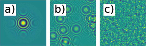
which shows how heterodyne speckles ultimately result from the sum of many independent single-particle contributions $s_j$, as depicted in Figure 2. Each single-particle contribution describes the self-referencing interference between the scattered spherical wave and the trans-illuminating beam. It exhibits circular fringes that become denser as the distance from the center of the pattern is increased, as sketched in Figure 2(a). These peculiar properties derive from probing the transmitted plane wave with a spherical wavefront [88] and they strongly rely on the mutual coherence between the two fields as ensured by the self-referencing scheme. Fringe visibility is progressively reduced by the angular distribution of the scattered light. The information on the complex scattered field is therefore conveyed by the amplitude and position of the interference fringes. Each single-particle interference image therefore represents the in-line hologram of the corresponding scattering particle.

Figure 2. Heterodyne speckles arise from the sum on an intensity basis of many equal single-particle interference patterns simply formed as in-line holograms of the scattering particles. Results of numerical computations obtained for (a) $N=1$, (b) $N=30$ and (c) $N={10}^5$

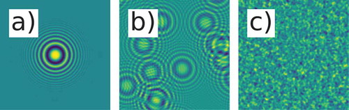
The self-referencing scheme is strongly reminiscent of in-line Gabor holography [84,89–91], originally proposed as a way to improve the resolution of the Transmission Electron Microscope (TEM) [92] and nowadays largely exploited in the visible range with laser light [93–96] or in the X-ray domain with coherent FEL beams [97–104]. The same self-referencing scheme is also at the basis of the Point Diffraction Interferometer (PDI) used in the X-ray community for phase-contrast imaging and wavefront characterization [99,105–109]. PDI also serves as a common-path interferometer for visible light applications [110–112].

2.2. Fourier-Optics-based theory of Heterodyne Near Field Speckles

Statistical analysis of Heterodyne Near Field Speckles is conveniently performed in the Fourier space [14–16], since the use of spatial power spectra allows to retrieve the interferometric information conveyed by the single-particle interferogram. As we will see, the power spectrum exhibits a well-defined appearance closely resembling the single-particle interference pattern itself, in contrast with the random look of the speckled intensity distribution. This will be particularly evident in Section 3 dealing with partially coherent radiation.

In Section 2.1 we have described the speckled intensity distribution as it would appear in a single frame. At variance, here we are interested in extracting the scattered signal $e_s$ from the static background $i_0$. By exploiting the continuous renewal of the sample ensured by the motion (either diffusive or collective) of the particles, this can be achieved without any additional blank measurement by subtracting two subsequent frames acquired at times $t$ and $t+\tau$, respectively (Double Frame Analysis, DFA [16]). The fluctuating differential heterodyne signal $\delta i(\mathbf{x},z,t,\tau )=i(\mathbf{x},z,t)-i(\mathbf{x},z,t+\tau )$ can thus be recovered and decomposed in its Fourier components (or plane waves). Adopting a common notation, quantities in the direct space and in the reciprocal space are labeled as $e(\mathbf{x})$ and $\hat{e}(\mathbf{q})$, respectively. Here we understand $\hat{e}(\mathbf{q})=\mathcal{F}\{e(\mathbf{x})\}(\mathbf{q})$, where $\mathcal{F}$ denotes a Fourier transform operation acting on $e(\mathbf{x})$ and $\mathbf{q}$ stands for the Fourier wave vectors, as opposed to the direct space variable $\mathbf{x}$. With reference to Figure 3, $\mathbf{q}$ is related to the scattering angle by $\mathbf{q}=k\theta$, as in standard interferometry [84].

Figure 3. (a) Scattering layout and (b) Fourier Optics approach to Heterodyne Near Field Speckles. Each Fourier component with wave vector q of heterodyne speckles arises from the interference of the intense trans-illuminating beam (thicker arrows) with the faint plane waves (thinner arrows) scattered by the sample along the symmetric wave vectors ±q

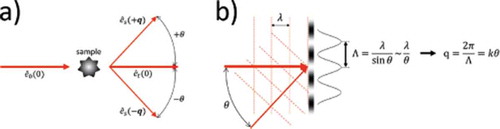
By recalling the convolution theorem of Fourier Optics, the Fourier transform of $\delta i$ takes the form:

(3) $\begin{array}{cc}\delta \hat{i}(\mathbf{q},z,t,\tau )& ={\hat{e}}_t(\mathbf{q})\otimes {\hat{e}}_s^{\ast }(-\mathbf{q},z,t)+{\hat{e}}_t^{\ast }(-\mathbf{q})\otimes {\hat{e}}_s(\mathbf{q},z,t)\\ \hspace{0.17em}& -{\hat{e}}_t(\mathbf{q})\otimes {\hat{e}}_s^{\ast }(-\mathbf{q},z,t+\tau )-{\hat{e}}_t^{\ast }(-\mathbf{q})\otimes {\hat{e}}_s(\mathbf{q},z,t+\tau ).\end{array}$(3)

Equation 3(3) $\begin{array}{cc}\delta \hat{i}(\mathbf{q},z,t,\tau )& ={\hat{e}}_t(\mathbf{q})\otimes {\hat{e}}_s^{\ast }(-\mathbf{q},z,t)+{\hat{e}}_t^{\ast }(-\mathbf{q})\otimes {\hat{e}}_s(\mathbf{q},z,t)\\ \hspace{0.17em}& -{\hat{e}}_t(\mathbf{q})\otimes {\hat{e}}_s^{\ast }(-\mathbf{q},z,t+\tau )-{\hat{e}}_t^{\ast }(-\mathbf{q})\otimes {\hat{e}}_s(\mathbf{q},z,t+\tau ).\end{array}$(3) and Figure 3 show that the Fourier components with wave vector $\mathbf{q}$ of heterodyne speckles arise from the interference between the transmitted beam and the three-dimensional plane waves scattered along the symmetric wave vectors ${\mathbf{k}}_s^{(+)}=(\mathbf{q},q_z)$ and ${\mathbf{k}}_s^{(-)}=(-\mathbf{q},q_z)$, where $q_z=(k^2-q^2{)}^{1/2}$ for elastic scattering and $q=|\mathbf{q}|$. Both waves contribute to the heterodyne signal [14–16].

Equation 3(3) $\begin{array}{cc}\delta \hat{i}(\mathbf{q},z,t,\tau )& ={\hat{e}}_t(\mathbf{q})\otimes {\hat{e}}_s^{\ast }(-\mathbf{q},z,t)+{\hat{e}}_t^{\ast }(-\mathbf{q})\otimes {\hat{e}}_s(\mathbf{q},z,t)\\ \hspace{0.17em}& -{\hat{e}}_t(\mathbf{q})\otimes {\hat{e}}_s^{\ast }(-\mathbf{q},z,t+\tau )-{\hat{e}}_t^{\ast }(-\mathbf{q})\otimes {\hat{e}}_s(\mathbf{q},z,t+\tau ).\end{array}$(3) also shows that $\delta \hat{i}$ conveys the information on the scattered field ${\hat{e}}_s$ through the convolution with ${\hat{e}}_t$. At variance, in the direct space, $e_t$ enters Equation 1(1) $i(\mathbf{x},z)\approx i_0(\mathbf{x})+e_t(\mathbf{x},z)e_s^{\ast }(\mathbf{x},z)+e_t^{\ast }(\mathbf{x},z)e_s(\mathbf{x},z)=i_0(\mathbf{x})+2\mathrm{\Re }\{e_t(\mathbf{x},z)e_s^{\ast }(\mathbf{x},z)\},$(1) through simple products between complex fields, namely as a local oscillator. The scattered field $e_s$ corresponds to fine-grain speckles, thus it exhibits spectral components over the whole range of spatial frequencies. Conversely, the transmitted incoming beam, which is endowed with a slowly-varying intensity distribution in the direct space, shows low-frequency components in the Fourier domain. We can therefore assume that the spectrum of the trans-illuminating beam ${\hat{e}}_t(\mathbf{q})$ is much narrower than the spectrum of the scattered light ${\hat{e}}_s(\mathbf{q})$. In the plane wave limit, where the field $e_t$ is uniform, ${\hat{e}}_t$ acts as a Dirac $\delta$-distribution in the convolution products. The power spectrum of the differential heterodyne signal $I=|\delta \hat{i}{|}^2$ then takes the form:

(4) $\begin{array}{cc}I(\mathbf{q},z,t,\tau )& =|{\hat{e}}_s^{\ast }(-\mathbf{q},z,t{)|}^2+|{\hat{e}}_s(\mathbf{q},z,t{)|}^2+|{\hat{e}}_s^{\ast }(-\mathbf{q},z,t+\tau {)|}^2+|{\hat{e}}_s(\mathbf{q},z,t+\tau {)|}^2\\ \hspace{0.17em}& -2\mathrm{\Re }\{{\hat{e}}_s(-\mathbf{q},z,t){\hat{e}}_s^{\ast }(-\mathbf{q},z,t+\tau )\}-2\mathrm{\Re }\{{\hat{e}}_s(\mathbf{q},z,t){\hat{e}}_s^{\ast }(\mathbf{q},z,t+\tau )\}\\ \hspace{0.17em}& +2\mathrm{\Re }\{{\hat{e}}_s(\mathbf{q},z,t){\hat{e}}_s(-\mathbf{q},z,t)\}+2\mathrm{\Re }\{{\hat{e}}_s(\mathbf{q},z,t+\tau ){\hat{e}}_s(-\mathbf{q},z,t+\tau )\}\\ \hspace{0.17em}& -2\mathrm{\Re }\{{\hat{e}}_s(-\mathbf{q},z,t){\hat{e}}_s(\mathbf{q},z,t+\tau )\}-2\mathrm{\Re }\{{\hat{e}}_s(\mathbf{q},z,t){\hat{e}}_s(-\mathbf{q},z,t+\tau )\}.\end{array}$(4)

Equation 4(4) $\begin{array}{cc}I(\mathbf{q},z,t,\tau )& =|{\hat{e}}_s^{\ast }(-\mathbf{q},z,t{)|}^2+|{\hat{e}}_s(\mathbf{q},z,t{)|}^2+|{\hat{e}}_s^{\ast }(-\mathbf{q},z,t+\tau {)|}^2+|{\hat{e}}_s(\mathbf{q},z,t+\tau {)|}^2\\ \hspace{0.17em}& -2\mathrm{\Re }\{{\hat{e}}_s(-\mathbf{q},z,t){\hat{e}}_s^{\ast }(-\mathbf{q},z,t+\tau )\}-2\mathrm{\Re }\{{\hat{e}}_s(\mathbf{q},z,t){\hat{e}}_s^{\ast }(\mathbf{q},z,t+\tau )\}\\ \hspace{0.17em}& +2\mathrm{\Re }\{{\hat{e}}_s(\mathbf{q},z,t){\hat{e}}_s(-\mathbf{q},z,t)\}+2\mathrm{\Re }\{{\hat{e}}_s(\mathbf{q},z,t+\tau ){\hat{e}}_s(-\mathbf{q},z,t+\tau )\}\\ \hspace{0.17em}& -2\mathrm{\Re }\{{\hat{e}}_s(-\mathbf{q},z,t){\hat{e}}_s(\mathbf{q},z,t+\tau )\}-2\mathrm{\Re }\{{\hat{e}}_s(\mathbf{q},z,t){\hat{e}}_s(-\mathbf{q},z,t+\tau )\}.\end{array}$(4) shows a remarkable symmetry. The first and the second lines involve products of conjugate fields scattered with the same wave vector (either $+\mathbf{q}$ or $-\mathbf{q}$), whereas the third and the fourth lines involve products of non-conjugate fields scattered at opposite wave vectors ($+\mathbf{q}$ and $-\mathbf{q}$). Furthermore, products between fields at the same time (either $t$ or $t+\tau$) appear in the first and in the third lines, whereas products of fields at different instants ($t$ and $t+\tau$) show in the second and in the fourth lines.

Interpretation of the four terms in the first line is straightforward. They represent products between conjugate fields at the same instant of time, thus by definition they convey the information on the scattered intensity distribution since the phases cancel. These terms are identical to each other for a stationary sample whose scattering properties do not vary in time. They are directly related to the particle form factor $S(\mathbf{q})$ under so-called deep Fresnel conditions (see Equation 5)(5) $z\ll \frac{Dd}{\lambda },$(5) .

Physical insight on the second, third and fourth lines comes by recalling some properties of the Fourier transform. Let $f(\mathbf{x})$ and $g(\mathbf{x})$ be two complex-valued functions and let us denote their Fourier transforms with $F(\mathbf{q})=\mathcal{F}\{f(\mathbf{x})\}(\mathbf{q})$ and $G(\mathbf{q})=\mathcal{F}\{g(\mathbf{x})\}(\mathbf{q})$, respectively. Following [84], the correlation (in real space) between $f(\mathbf{x})$ and $g(\mathbf{x})$ is the product $F(\mathbf{q})G^{\ast }(\mathbf{q})$ in Fourier space, whereas the convolution (in real space) between $f(\mathbf{x})$ and $g(\mathbf{x})$ is the product $F(\mathbf{q})G(\mathbf{q})$ in Fourier space. We notice that, in both cases, $F$ and $G$ are evaluated at the same $\mathbf{q}$, and that a complex conjugate appears in the case of correlations.

The terms in the second line are in the form $F(\mathbf{q})G^{\ast }(\mathbf{q})$, thus they describe correlations. Since in this case both $F$ and $G$ are equal to the Fourier transform of the complex scattered field ${\hat{e}}_s$, though at different times, they describe the effects of the spatial correlations between the two frames on the scattered intensity distribution. Interestingly, these terms carry the information on the dynamics of the system (see below).

Products appearing in the third and in the fourth lines are of the type $F(\mathbf{q})G(-\mathbf{q})$. Despite they might resemble the Fourier space representation of convolutions, they actually describe correlations due to the $-\mathbf{q}$ in $G$. Indeed, these products can be cast in the form $F(\mathbf{q})H^{\ast }(\mathbf{q})$ by means of the general relation $G(-\mathbf{q})=\mathcal{F}\{g(\mathbf{x})\}(-\mathbf{q})=[\mathcal{F}\{g^{\ast }(\mathbf{x})\}(\mathbf{q}){]}^{\ast }$ and by introducing $H(\mathbf{q})=\mathcal{F}\{g^{\ast }(\mathbf{x})\}(\mathbf{q})$. Therefore, they describe the correlations between the scattered field and its complex conjugate, namely between the fields scattered along, and coming from, opposite directions. These terms are responsible for deep oscillations in the low-q region of the spectrum, also known as Talbot oscillations. In terms of Fourier Optics, Talbot oscillations arise from the finite correlations between the plane waves scattered at $+\mathbf{q}$ and $-\mathbf{q}$ (see Section 2.3) and they vanish if the correlations are lost (see Sections 2.3.1 and 2.3.2). This is particularly evident from the terms in the third line, where the fields are evaluated at the same instant of time. The terms in the fourth line, involving fields at different times, describe how the amplitude of the Talbot oscillations is reduced by the finite correlations between subsequent frames.

To further develop Equation 4(4) $\begin{array}{cc}I(\mathbf{q},z,t,\tau )& =|{\hat{e}}_s^{\ast }(-\mathbf{q},z,t{)|}^2+|{\hat{e}}_s(\mathbf{q},z,t{)|}^2+|{\hat{e}}_s^{\ast }(-\mathbf{q},z,t+\tau {)|}^2+|{\hat{e}}_s(\mathbf{q},z,t+\tau {)|}^2\\ \hspace{0.17em}& -2\mathrm{\Re }\{{\hat{e}}_s(-\mathbf{q},z,t){\hat{e}}_s^{\ast }(-\mathbf{q},z,t+\tau )\}-2\mathrm{\Re }\{{\hat{e}}_s(\mathbf{q},z,t){\hat{e}}_s^{\ast }(\mathbf{q},z,t+\tau )\}\\ \hspace{0.17em}& +2\mathrm{\Re }\{{\hat{e}}_s(\mathbf{q},z,t){\hat{e}}_s(-\mathbf{q},z,t)\}+2\mathrm{\Re }\{{\hat{e}}_s(\mathbf{q},z,t+\tau ){\hat{e}}_s(-\mathbf{q},z,t+\tau )\}\\ \hspace{0.17em}& -2\mathrm{\Re }\{{\hat{e}}_s(-\mathbf{q},z,t){\hat{e}}_s(\mathbf{q},z,t+\tau )\}-2\mathrm{\Re }\{{\hat{e}}_s(\mathbf{q},z,t){\hat{e}}_s(-\mathbf{q},z,t+\tau )\}.\end{array}$(4) , we describe the scattering sample as a weak phase object with no absorption. To a first-order approximation [84], the complex field just downstream the sample is therefore given by $1+ia\mathrm{\Phi }(\mathbf{x},t)$ for the case of a uniform incident field with unitary amplitude. Notice how this expression is entirely equivalent to the heterodyne conditions. Here $a\mathrm{\Phi }(\mathbf{x},t)$, with $a\ll 1$, is the random phase modulation induced by the sample on the incident beam at time $t$. It is ultimately responsible for the scattered field $e_s$. The intensity at the observation plane is obtained by propagating the complex field just downstream the sample over a distance $z$. In the real space, propagation is described as the convolution with the propagator $exp[ik{x}^2/(2z)]$, namely a spherical wave. In the Fourier space, each Fourier component of the complex field with wave vector $q$ is therefore multiplied by $exp[-iz{q}^2/(2k)]$ [84]. It is then straightforward to derive an expression for the Fourier transform of the resulting intensity distribution at the observation plane at time $t$ as $\hat{i}(\mathbf{q},z,t)=\delta (\mathbf{q})+2sin[z{q}^2/(2k)]e_s(\mathbf{q},z,t)$. The oscillating function describes the Talbot oscillations introduced below Equation 4(4) $\begin{array}{cc}I(\mathbf{q},z,t,\tau )& =|{\hat{e}}_s^{\ast }(-\mathbf{q},z,t{)|}^2+|{\hat{e}}_s(\mathbf{q},z,t{)|}^2+|{\hat{e}}_s^{\ast }(-\mathbf{q},z,t+\tau {)|}^2+|{\hat{e}}_s(\mathbf{q},z,t+\tau {)|}^2\\ \hspace{0.17em}& -2\mathrm{\Re }\{{\hat{e}}_s(-\mathbf{q},z,t){\hat{e}}_s^{\ast }(-\mathbf{q},z,t+\tau )\}-2\mathrm{\Re }\{{\hat{e}}_s(\mathbf{q},z,t){\hat{e}}_s^{\ast }(\mathbf{q},z,t+\tau )\}\\ \hspace{0.17em}& +2\mathrm{\Re }\{{\hat{e}}_s(\mathbf{q},z,t){\hat{e}}_s(-\mathbf{q},z,t)\}+2\mathrm{\Re }\{{\hat{e}}_s(\mathbf{q},z,t+\tau ){\hat{e}}_s(-\mathbf{q},z,t+\tau )\}\\ \hspace{0.17em}& -2\mathrm{\Re }\{{\hat{e}}_s(-\mathbf{q},z,t){\hat{e}}_s(\mathbf{q},z,t+\tau )\}-2\mathrm{\Re }\{{\hat{e}}_s(\mathbf{q},z,t){\hat{e}}_s(-\mathbf{q},z,t+\tau )\}.\end{array}$(4) . It ultimately results from the Fourier transform of the near field propagator under heterodyne conditions, namely from the Fourier transform of the interference pattern generated by a spherical wave and a plane wavefront, as we will remark in Section 2.3.

In so-called deep near field conditions (or deep Fresnel regime) [113–114], given by

(5) $z\ll \frac{Dd}{\lambda },$(5)

the relation $|e_s(\mathbf{q},z,t){|}^2=S(\mathbf{q})$ is valid, thus yielding the following expression (equivalent to Equation 4)(4) $\begin{array}{cc}I(\mathbf{q},z,t,\tau )& =|{\hat{e}}_s^{\ast }(-\mathbf{q},z,t{)|}^2+|{\hat{e}}_s(\mathbf{q},z,t{)|}^2+|{\hat{e}}_s^{\ast }(-\mathbf{q},z,t+\tau {)|}^2+|{\hat{e}}_s(\mathbf{q},z,t+\tau {)|}^2\\ \hspace{0.17em}& -2\mathrm{\Re }\{{\hat{e}}_s(-\mathbf{q},z,t){\hat{e}}_s^{\ast }(-\mathbf{q},z,t+\tau )\}-2\mathrm{\Re }\{{\hat{e}}_s(\mathbf{q},z,t){\hat{e}}_s^{\ast }(\mathbf{q},z,t+\tau )\}\\ \hspace{0.17em}& +2\mathrm{\Re }\{{\hat{e}}_s(\mathbf{q},z,t){\hat{e}}_s(-\mathbf{q},z,t)\}+2\mathrm{\Re }\{{\hat{e}}_s(\mathbf{q},z,t+\tau ){\hat{e}}_s(-\mathbf{q},z,t+\tau )\}\\ \hspace{0.17em}& -2\mathrm{\Re }\{{\hat{e}}_s(-\mathbf{q},z,t){\hat{e}}_s(\mathbf{q},z,t+\tau )\}-2\mathrm{\Re }\{{\hat{e}}_s(\mathbf{q},z,t){\hat{e}}_s(-\mathbf{q},z,t+\tau )\}.\end{array}$(4) for the power spectrum of the differential heterodyne signal:

(6) $\begin{array}{cc}I(\mathbf{q},z,t,\tau )& =4\left[2{sin}^2\left(\frac{z{q}^2}{2k}\right)\right]\left[S(\mathbf{q})-\mathrm{\Re }\{e_s(\mathbf{q},z,t)e_s^{\ast }(\mathbf{q},z,t+\tau )\}\right]\\ \hspace{0.17em}& =4T(q,z)\left[S(\mathbf{q})-\mathrm{\Re }\{e_s(\mathbf{q},z,t)e_s^{\ast }(\mathbf{q},z,t+\tau )\}\right],\end{array}$(6)

where $T(q,z)$ describes the Talbot oscillations in the power spectrum and it is known as the Talbot transfer function. It ultimately describes how the phase difference between the two waves scattered at $+\mathbf{q}$ and $-\mathbf{q}$ changes as a function of $q$ and $z$ (see discussion below Equation 4)(4) $\begin{array}{cc}I(\mathbf{q},z,t,\tau )& =|{\hat{e}}_s^{\ast }(-\mathbf{q},z,t{)|}^2+|{\hat{e}}_s(\mathbf{q},z,t{)|}^2+|{\hat{e}}_s^{\ast }(-\mathbf{q},z,t+\tau {)|}^2+|{\hat{e}}_s(\mathbf{q},z,t+\tau {)|}^2\\ \hspace{0.17em}& -2\mathrm{\Re }\{{\hat{e}}_s(-\mathbf{q},z,t){\hat{e}}_s^{\ast }(-\mathbf{q},z,t+\tau )\}-2\mathrm{\Re }\{{\hat{e}}_s(\mathbf{q},z,t){\hat{e}}_s^{\ast }(\mathbf{q},z,t+\tau )\}\\ \hspace{0.17em}& +2\mathrm{\Re }\{{\hat{e}}_s(\mathbf{q},z,t){\hat{e}}_s(-\mathbf{q},z,t)\}+2\mathrm{\Re }\{{\hat{e}}_s(\mathbf{q},z,t+\tau ){\hat{e}}_s(-\mathbf{q},z,t+\tau )\}\\ \hspace{0.17em}& -2\mathrm{\Re }\{{\hat{e}}_s(-\mathbf{q},z,t){\hat{e}}_s(\mathbf{q},z,t+\tau )\}-2\mathrm{\Re }\{{\hat{e}}_s(\mathbf{q},z,t){\hat{e}}_s(-\mathbf{q},z,t+\tau )\}.\end{array}$(4) .

The quantity $I(\mathbf{q},z,t,\tau )$ is referred to as the intermediate scattering function [16,20]. If the frames are correlated, it brings the information on the sample dynamics, as the last product represents the spatio-temporal correlations of the scattered field. It yields invaluable information either on the sample dynamics (diffusive motion) or on collective motions (sedimentation, convection, forced flow). In the first case, dynamic light scattering measurements are possible (see Section 2.4.2). In the second case, speckle fields can be exploited to implement a velocimetry technique (see Section 2.4.3). The same principles can be applied to track speckle motions induced by changes in the incoming wavefront, with straightforward applications to wavefront sensing (see Section 4.3) and phase-contrast imaging (see Section 4.4).

Conversely, if the frames are uncorrelated, and in the absence of Talbot oscillations (see Section 2.3.1 and 2.3.2), the intermediate scattering function reduces to

(7) $I(\mathbf{q},z)=4S(\mathbf{q}),$(7)

thus enabling direct measurements of the particle form factor. Equations 5(5) $z\ll \frac{Dd}{\lambda },$(5) and 7(7) $I(\mathbf{q},z)=4S(\mathbf{q}),$(7) describe the Heterodyne Near Field Scattering (HNFS) regime introduced by Giglio and co-workers [14–16]. It allows to directly gauge the information on the scattering sample from deep near field speckles, regardless of the observation distance $z$. Notice how Equation 5(5) $z\ll \frac{Dd}{\lambda },$(5) is more stringent than the usual Fresnel conditions $z\ll D^2/\lambda$. The power spectrum of heterodyne speckles is independent on $z$ in deep Fresnel conditions and it equals the particle form factor. As a consequence, the speckle size is equal to the size of the scatterers and it is independent on the distance from the scattering sample and the wavelength, a remarkable property for an interference phenomenon [113,114]. Indeed, the speckle size can be estimated from the width of the field autocorrelation function. By means of the Wiener-Khinchin theorem of statistical optics [9–11], the latter is computed by Fourier transforming Equation 7(7) $I(\mathbf{q},z)=4S(\mathbf{q}),$(7) , thus $ACF(\mathbf{x},z)\propto \mathcal{F}\{S(\mathbf{q})\}(\mathrm{\Delta }\mathbf{x})$. It has a characteristic width given by $d_{sp}=2\pi /q^{\ast }=2\pi /(k{\theta }^{\ast })=d$ where $q^{\ast }$ represents the characteristic width of $S(\mathbf{q})$ and ${\theta }^{\ast }=\lambda /d$ is the scattering angle for particles with diameter $d$. Examples of Heterodyne Near Field Speckles from two different colloidal samples with diameter $d=5$ $\mu$m and $d=10$ $\mu$m, respectively, are shown in Figure 4.

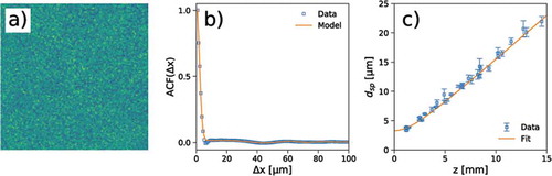
Figure 4. Heterodyne Near Field Speckles obtained with coherent light from ensembles of particles with average diameter (a,c) $d=5$ $\mu$m and (b,d) $d=10$ $\mu$m at two different distances (a,b) $z_1=1$ mm and (c,d) $z_2=2$ mm downstream the sample. Each square is 150 × 150 $\mu$m${ }^2$ in real space. The average speckle size does not vary with $z$ and it matches the size of the scatterers

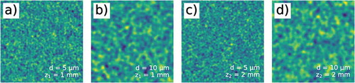
2.3. The Talbot oscillations

When the plane waves scattered at $+\mathbf{q}$ and $-\mathbf{q}$ are correlated, the power spectrum of Heterodyne Near Field Speckles exhibits deep Talbot oscillations [14–16]. For temporally uncorrelated frames, Equation 7(7) $I(\mathbf{q},z)=4S(\mathbf{q}),$(7) then takes the form:

(8) $I(\mathbf{q},z)=4T(q,z)S(\mathbf{q})=4\left[2{sin}^2\left(\frac{z{q}^2}{2k}\right)\right]S(\mathbf{q}).$(8)

Opposite to the HNFS regime of Equation 7(7) $I(\mathbf{q},z)=4S(\mathbf{q}),$(7) , the power spectrum in Equation 8(8) $I(\mathbf{q},z)=4T(q,z)S(\mathbf{q})=4\left[2{sin}^2\left(\frac{z{q}^2}{2k}\right)\right]S(\mathbf{q}).$(8) is affected by the rather complicate Talbot transfer function $T(q,z)$. In particular, a large minimum is present around $q=0$, as well as multiple zeros at higher wave vectors.

Equation 8(8) $I(\mathbf{q},z)=4T(q,z)S(\mathbf{q})=4\left[2{sin}^2\left(\frac{z{q}^2}{2k}\right)\right]S(\mathbf{q}).$(8) is typical of the Raman-Nath scattering regime, where ${\hat{e}}_s(\mathbf{q})$ and ${\hat{e}}_s(-\mathbf{q})$ are scattered by a weak, purely 2D (i.e. thin) sinusoidal phase grating [84]. For such a system, the interference of ${\hat{e}}_s(\mathbf{q})$ and ${\hat{e}}_s(-\mathbf{q})$ with the trans-illuminating beam in the near field is at the basis of the well-known Talbot self-imaging phenomenon, namely the appearance in the resulting intensity distribution of exact replica of the sinusoidal grating. The contrast of such self-images (equivalently, the corresponding power spectrum) varies as a function of $z$ and $q$ according to the Talbot transfer function $T(q,z)=2{sin}^2[z{q}^2/(2k)]$. In the general case of a random weak phase object, Talbot oscillations appear in the power spectrum of the resulting self-referencing speckles. Therefore, Talbot oscillations ultimately describe the modulations of the interference between the weak scattered waves and the trans-illuminating beam. It is the regime where quantitative shadowgraphy [115] and X-ray phase-contrast imaging [116–118] are operated. In the X-ray community, $T(q,z)$ is also referred to as the phase contrast trasfer function [118].

We emphasize that, in the Raman-Nath scattering regime, the Talbot transfer function is the Fourier-space representation of the interference between a plane wave and a spherical wavefront, namely the power spectrum of the hologram of a spherical wave [30]. Thus, Talbot oscillations in the power spectrum of heterodyne speckles are the peculiar signature of the interference pattern produced by a particle in the self-referencing scheme. Notice that such an interference pattern actually resembles the hologram of a spherical wave, but only for very small and optically soft particles, for which the scattered spherical wave is perfectly phased with the transmitted plane wavefront [119]. In the most general case, according to the Optical Theorem [119], the phase lag $\varphi$ of the scattered wave with respect to the incident wave transforms $T(q,z)$ into $T(q,z,\varphi )=2{sin}^2[z{q}^2/(2k)-\varphi ]$. This means that Talbot oscillations become sample-dependent, which in turns remarkably implies the possibility of simultaneously accessing both the modulus and the phase of the forward scattering amplitude [24,120].

In Equation 6(6) $\begin{array}{cc}I(\mathbf{q},z,t,\tau )& =4\left[2{sin}^2\left(\frac{z{q}^2}{2k}\right)\right]\left[S(\mathbf{q})-\mathrm{\Re }\{e_s(\mathbf{q},z,t)e_s^{\ast }(\mathbf{q},z,t+\tau )\}\right]\\ \hspace{0.17em}& =4T(q,z)\left[S(\mathbf{q})-\mathrm{\Re }\{e_s(\mathbf{q},z,t)e_s^{\ast }(\mathbf{q},z,t+\tau )\}\right],\end{array}$(6) , decorrelations between the fields scattered at $+\mathbf{q}$ and $-\mathbf{q}$ are induced by the dynamics of the sample, as evidenced by the interference-like products between fields at different times in Equation 4(4) $\begin{array}{cc}I(\mathbf{q},z,t,\tau )& =|{\hat{e}}_s^{\ast }(-\mathbf{q},z,t{)|}^2+|{\hat{e}}_s(\mathbf{q},z,t{)|}^2+|{\hat{e}}_s^{\ast }(-\mathbf{q},z,t+\tau {)|}^2+|{\hat{e}}_s(\mathbf{q},z,t+\tau {)|}^2\\ \hspace{0.17em}& -2\mathrm{\Re }\{{\hat{e}}_s(-\mathbf{q},z,t){\hat{e}}_s^{\ast }(-\mathbf{q},z,t+\tau )\}-2\mathrm{\Re }\{{\hat{e}}_s(\mathbf{q},z,t){\hat{e}}_s^{\ast }(\mathbf{q},z,t+\tau )\}\\ \hspace{0.17em}& +2\mathrm{\Re }\{{\hat{e}}_s(\mathbf{q},z,t){\hat{e}}_s(-\mathbf{q},z,t)\}+2\mathrm{\Re }\{{\hat{e}}_s(\mathbf{q},z,t+\tau ){\hat{e}}_s(-\mathbf{q},z,t+\tau )\}\\ \hspace{0.17em}& -2\mathrm{\Re }\{{\hat{e}}_s(-\mathbf{q},z,t){\hat{e}}_s(\mathbf{q},z,t+\tau )\}-2\mathrm{\Re }\{{\hat{e}}_s(\mathbf{q},z,t){\hat{e}}_s(-\mathbf{q},z,t+\tau )\}.\end{array}$(4) . Thus the refresh of the statistical ensemble affects the amplitude of Talbot oscillations in Equation 6(6) $\begin{array}{cc}I(\mathbf{q},z,t,\tau )& =4\left[2{sin}^2\left(\frac{z{q}^2}{2k}\right)\right]\left[S(\mathbf{q})-\mathrm{\Re }\{e_s(\mathbf{q},z,t)e_s^{\ast }(\mathbf{q},z,t+\tau )\}\right]\\ \hspace{0.17em}& =4T(q,z)\left[S(\mathbf{q})-\mathrm{\Re }\{e_s(\mathbf{q},z,t)e_s^{\ast }(\mathbf{q},z,t+\tau )\}\right],\end{array}$(6) . Here we would like to stress that the mutual correlation between the two symmetrically scattered waves ${\hat{e}}_s(\mathbf{q})$ and ${\hat{e}}_s(-\mathbf{q})$, responsible of the Talbot oscillations, might be reduced by other effects even for uncorrelated frames. As a result, the Talbot oscillations in power spectra eventually vanish, leading to Equation 7(7) $I(\mathbf{q},z)=4S(\mathbf{q}),$(7) . In the forthcoming sections, we will deal with the two most common effects: scattering from a 3D sample and the finite size of the detection screen.

2.3.1. The modified Talbot transfer function: 3D scattering

Let us consider the scattering from a three-dimensional object with thickness $l$. Density fluctuations occur within each thin layer of randomly displaced particles. For what concerns light scattering, each Fourier mode of such random fluctuations acts as a thin sinusoidal phase grating, thus scattering a pair of correlated waves at $+\mathbf{q}$ and $-\mathbf{q}$ in the Raman-Nath regime (see Section 2.3). The total fields ${\hat{e}}_s(\mathbf{q})$ and ${\hat{e}}_s(-\mathbf{q})$ emerging from the sample result from the superposition of such elementary contributions, as shown in Figure 5(a). Owing to the stochastic nature of the sample, the different phase gratings are generally randomly displaced one with respect to others. Thus, by virtue of the shift theorem of Fourier Optics [84], the elementary contributions from each thin layer add up with random phases and the correlation between ${\hat{e}}_s(\mathbf{q})$ and ${\hat{e}}_s(-\mathbf{q})$ vanishes. An alternative description comes by considering that scattering from a three-dimensional object can be interpreted as Bragg reflection. Only one wave is scattered, either at $+\mathbf{q}$ or $-\mathbf{q}$, and the Talbot oscillations do not form [15].

Figure 5. (a) Fourier Optics approach and (b) direct space approach to (c) the effects of Bragg-like scattering from a 3D sample on the Talbot oscillations. The Talbot oscillations are reported as a function of the reduced Fourier wave vector $q/q_{3D}$ (see text for a definition of $q_{3D}$). From plot (a), the density fluctuations occurring within each thin layer of randomly displaced particles are decomposed into Fourier modes. Each Fourier mode acts as a thin sinusoidal phase grating scattering a pair of correlated waves at $+\mathbf{q}$ and $-\mathbf{q}$. These elementary contributions from the different $n$ layers add up with random phases $exp[i{\varphi }_j^{(+)}]$ and $exp[i{\varphi }_j^{(-)}]$ for $j=1\cdots n$ along the $+\mathbf{q}$ and $-\mathbf{q}$ directions, respectively. Their incoherent sum is effective in reducing the correlation between the emerging waves ${\hat{e}}_s(\mathbf{q})$ and ${\hat{e}}_s(-\mathbf{q})$. Parameters of simulations: $\lambda =0.1$ nm, $z=50$ cm, $l=10$ cm

A description in real space is also possible. Particles located at different $z$ generate interference fringes with different spacings, as shown in Figure 5(b). The superposition of the corresponding Talbot oscillations in the power spectrum eventually results in partial or total cancellation [21]:

(9) $T_{3D}(q,z)=\frac{1}{l}{\int }_{z-l/2}^{z-l/2}T(q,z{ }^{\mathrm{\prime }})\mathrm{d}z{ }^{\mathrm{\prime }}=1-cos\left(\frac{z{q}^2}{k}\right)\mathrm{s}\mathrm{i}\mathrm{n}\mathrm{c}\left(\frac{l{q}^2}{2k}\right).$(9)

Talbot oscillations are highly suppressed for $q>q_{3D}=(2\pi k/l{)}^{1/2}$, as reported in Figure 5(c). Thus, below $q_{3D}$, the system can be regarded as a 2D object exhibiting Talbot oscillations, whereas it behaves as a 3D object for higher wave vectors.

2.3.2. The modified Talbot transfer function: walkoff effect

Decorrelation between ${\hat{e}}_s(\mathbf{q})$ and ${\hat{e}}_s(-\mathbf{q})$ might also occur due to the finite size $L$ of the detection screen [120]. In this case, the two scattered waves originate from two partially-overlapping regions on the scattering plane, obtained by geometrical back-projection of the finite screen along the ${\mathbf{k}}_s^{(+)}$ and ${\mathbf{k}}_s^{(-)}$ directions, as shown in Figure 6(a). Therefore, ${\hat{e}}_s(\mathbf{q})$ and ${\hat{e}}_s(-\mathbf{q})$ are not totally correlated due to the random contributions from non-overlapping regions of the sample.

Figure 6. (a) Fourier Optics approach and (b) direct space approach to (c) the effects of the finite sensor size on the Talbot oscillations. The Talbot oscillations are reported as a function of the reduced Fourier wave vector $q/q_{wo}$ (see text for a definition of $q_{wo}$). From plot (a), it can be seen that $\beta$ in Equation 10(10) $T_{wo}(q,z)=\left\{\begin{array}{cc}1+\beta (q,z)\left[T(q,z)-1\right]& q\le q_{wo}\\ 1& q>q_{wo}\end{array}\right.\beta (q,z)=\frac{L-2qz/k}{L+2qz/k},$(10) is given by $\beta =A/B$, namely the ratio between the volume of the sample that scatters correlated waves at $\pm \mathbf{q}$ and the total volume of the sample intercepted by back-propagating the sensor with finite size $L$ along the ${\mathbf{k}}_s^{(\pm )}$ directions. Parameters of simulations: $\lambda =0.1$ nm, $z=50$ cm, $L=33\mu$m

In the real-space, a finite screen collects mostly incomplete fringes [120], as depicted in Figure 6(b). One can show that incomplete fringes contribute to the power spectrum but do not generate Talbot oscillations [120]:

(10) $T_{wo}(q,z)=\left\{\begin{array}{cc}1+\beta (q,z)\left[T(q,z)-1\right]& q\le q_{wo}\\ 1& q>q_{wo}\end{array}\right.\beta (q,z)=\frac{L-2qz/k}{L+2qz/k},$(10)

with $q_{wo}=kL/(2z)$. As shown in Figure 6(c), Talbot oscillations are progressively tapered and they eventually vanish for $q>q_{wo}$.

2.4. Applications of Heterodyne Near Field Speckles

2.4.1. Static low-angle scattering

Recalling what stated in Section 2.2, Heterodyne Near Field Speckles can be exploited for particle sizing, as the speckle size equals the size of the scatterers in deep near field conditions. Different samples can therefore be compared by simple visual inspection of raw images [18], as also shown in Figure 4. Quantitative information on the scattered field, thus on the particles themselves, is directly extracted from the speckle autocorrelation function since the measured intensity is directly proportional to $e_s$. Notice how qualitative comparisons between different samples are also possible with homodyne speckles if the deep near field conditions are fulfilled [113,114]. However, a quantitative analysis based on speckle autocorrelation functions is not as straightforward as in the heterodyne case and particular processing techniques must be implemented, as thoroughly detailed in [114].

The particle form factor is directly accessed from the measured power spectrum in the HNFS regime of Equation 7(7) $I(\mathbf{q},z)=4S(\mathbf{q}),$(7) free from Talbot oscillations, the latter being removed by exploiting either the 3D scattering from a thick sample (see Section 2.3.1) or the walkoff effect induced by a finite sensor (see Section 2.3.2). Successful measurements have been performed on calibrated spherical colloids with diameter in the range 1 $\mu$m to 10 $\mu$m [14–16,18]. Data for monodisperse [14–16,18] as well as bimodal suspensions [15,16] have been reported. They agree remarkably well with Mie predictions [119] and with results from state-of-the-art Small-Angle Light Scattering (SALS) apparatus, though over an appreciably extended $q$ range. The accessible $q$ range typically spans two to three orders of magnitude from $q_{\mathrm{m}\mathrm{i}\mathrm{n}}=2\pi M/L$ to $q_{\mathrm{m}\mathrm{a}\mathrm{x}}=2\pi M/(2d_{\mathrm{p}\mathrm{x}\mathrm{l}})$ (Nyquist frequency), being $L=N{d}_{\mathrm{p}\mathrm{x}\mathrm{l}}$ the sensor size, $N$ the number of pixels, $d_{\mathrm{p}\mathrm{x}\mathrm{l}}$ the pixel size and $M$ the magnification of the relay optics. Typical values are $q_{\mathrm{m}\mathrm{i}\mathrm{n}}=0.025$ $\mu$m${ }^{-1}$ and $q_{\mathrm{m}\mathrm{a}\mathrm{x}}=12.5$ $\mu$m${ }^{-1}$ for $M=20$, $N=1000$ and $d_{\mathrm{p}\mathrm{x}\mathrm{l}}=5$ $\mu$m, though in practice $q_{\mathrm{m}\mathrm{a}\mathrm{x}}$ might be actually limited by e.g. the numerical aperture of the optics.

Polydispersity is easier to analyze with respect to the earlier Near Field Scattering (NFS) method based on homodyne speckles [113,114]. This capability derives from HNFS being linear in the scattered fields, at variance with the homodyne case where the analysis is complicated by cross terms in the homodyne spectrum.

A comparative study on the sensitivity of the technique against SALS experiments has also been performed [16]. Samples with progressively decreasing volume fractions from ${10}^{-5}$ to ${10}^{-8}$ were investigated, and the HNFS method proved more reliable in retrieving the particle form factor even at the lowest concentrations.

The HNFS technique has been exploited to characterize the power spectrum of large scale non-equilibrium fluctuations (on the millimeter scale, corresponding to a characteristic Fourier wave vector of $0.006$ $\mu$m${ }^{-1}$) during a free-diffusion process in binary mixtures [17]. To access such ultra-low scattering angles, a setup based on a Schlieren-like spatial filter has been designed to rigorously generate a flat transfer function over the entire $q$-range. At variance, quantitative shadowgraphy [115] suffers from deep modulations introduced by the Talbot transfer function.

The fast data analysis of the HNFS technique also allows quasi-real-time measurements. By continuously analyzing power spectra during the free diffusion process, the evolution of the roll-off wave vector was followed, which is known to yield valuable information on the temporal evolution of the concentration gradient [17,121]. The same analysis allows to monitor the kinetics of non-stationary systems, such as aggregating colloids forming fractal structures [16].

Recently, Heterodyne Near Field Speckles have been applied to characterize colloidal samples under forced flow [24]. The sample is illuminated by a thin light sheet perpendicular to the flow direction to minimize the transit times of the particles. Speckle contrast is also enhanced thanks to the intense illumination provided by the tight vertical focusing. Sensitivity to small signals is therefore highly improved. By properly choosing the sample thickness, the static form factor of spherical particles and colloidal aggregates was measured for $q>q_{3D}$ (refer to Equation 9(9) $T_{3D}(q,z)=\frac{1}{l}{\int }_{z-l/2}^{z-l/2}T(q,z{ }^{\mathrm{\prime }})\mathrm{d}z{ }^{\mathrm{\prime }}=1-cos\left(\frac{z{q}^2}{k}\right)\mathrm{s}\mathrm{i}\mathrm{n}\mathrm{c}\left(\frac{l{q}^2}{2k}\right).$(9) ), whereas Talbot oscillations at lower $q$ conveyed the information of the phase lag $\varphi$ of the zero-angle scattered wave [120].

We finally stress how the light sheet illumination adopted in ref [24]. poses interesting questions on the nature of the near field. Referring to Equation 5(5) $z\ll \frac{Dd}{\lambda },$(5) , far field conditions immediately set in along the focusing direction since $D$ is of the order of a few microns. Contrarily, deep near field conditions are fulfilled along the orthogonal direction thanks to the large beam diameter. At the sensor plane, degenerate far field speckles are registered along the focusing direction, while genuine deep Fresnel speckles develop along the orthogonal direction. We will encounter similar conditions in Section 4.1 and Section 4.2 with undulator X-ray beams endowed with elongated coherence areas. We will see how the arguments developed here and in Section 2.2 still apply with partially coherent radiation by replacing $D$, the diameter of the coherent wavefront, with ${\sigma }_{\mathrm{c}\mathrm{o}\mathrm{h}}$, the size of the coherence patches. This proves that the concept of near field is related to the coherent portion of the illuminating wavefront. In particular, equivalence is found between partially coherent radiation whose statistical properties (the coherence areas) are described by a given spatial coherence function and the case of a fully coherent wavefront with an intensity distribution determined by the very same function.

2.4.2. Dynamic low-angle scattering

The Heterodyne Near Field Speckle technique, originally conceived for static low-angle scattering measurements, also provides dynamic data through the intermediate scattering function of Equation (6)(6) $\begin{array}{cc}I(\mathbf{q},z,t,\tau )& =4\left[2{sin}^2\left(\frac{z{q}^2}{2k}\right)\right]\left[S(\mathbf{q})-\mathrm{\Re }\{e_s(\mathbf{q},z,t)e_s^{\ast }(\mathbf{q},z,t+\tau )\}\right]\\ \hspace{0.17em}& =4T(q,z)\left[S(\mathbf{q})-\mathrm{\Re }\{e_s(\mathbf{q},z,t)e_s^{\ast }(\mathbf{q},z,t+\tau )\}\right],\end{array}$(6) . It allows to gauge the temporal correlation function of the scattered field at all $q$ simultaneously, hence the diffusion coefficient of the scatterers [122]. For Brownian samples, the diameters of the particles can therefore be accurately recovered by means of the the Stokes-Einstein relation [20].

Remarkably, the possibility of performing simultaneous static and dynamic scattering measurements has been exploited in the Near Field Scattering unit of the Selectable Optical Diagnostic Instrument (SODI) on board the International Space Station (ISS) [21,22]. In microgravity conditions, aggregation of colloidal particles has been driven by critical Casimir forces, in absence of any convection and sedimentation [123–125]. By strongly suppressing any buoyancy-driven flow, the true Brownian and rotational motions of the growing aggregates have been probed for the first time [21,22,125]. By independently measuring the radius of gyration and the hydrodynamic radius, useful insight is gained on the structure and compactness of the fractal aggregates. Surprisingly, it has been evidenced that the mass is always evenly distributed in all objects [22]. This was also confirmed by holographic reconstruction of the clusters from the very same speckle images [22]. This possibility strongly relies on the linearity of the measured intensity with respect to the scattered field, allowing to gauge both amplitude and phase information.

Recently, the capability of HNFS of performing static and dynamic scattering measurements on turbid samples has been investigated [23]. A generalized version of Equation 6(6) $\begin{array}{cc}I(\mathbf{q},z,t,\tau )& =4\left[2{sin}^2\left(\frac{z{q}^2}{2k}\right)\right]\left[S(\mathbf{q})-\mathrm{\Re }\{e_s(\mathbf{q},z,t)e_s^{\ast }(\mathbf{q},z,t+\tau )\}\right]\\ \hspace{0.17em}& =4T(q,z)\left[S(\mathbf{q})-\mathrm{\Re }\{e_s(\mathbf{q},z,t)e_s^{\ast }(\mathbf{q},z,t+\tau )\}\right],\end{array}$(6) is derived to account for moderate multiple scattering in the intermediate scattering function. It is reported that reliable values of the particle size can be obtained for transmissions of the sample down to 0.7 (typically, the Heterodyne Near Field Speckle method is operated with transmissions larger than 0.9). It is also evidenced that this possibility is strongly connected to the small scattering wave vectors accessed by the technique [14–16]. Indeed, small $q$-values correspond to large length scales with relatively slow dynamics [122], therefore faster fluctuations caused by strong multiple scattering are not sensed.

The reader can refer to [126] on near field scattering techniques, discussing and reviewing earlier developments of the Heterodyne Near Field Speckle method aimed at static and dynamic light scattering measurements. Besides this, it also describes advanced near-field optical techniques linking the scattering and the imaging approaches, thus enabling local characterizations of the samples as well.

2.4.3. Velocimetry

Heterodyne Near Field Speckles can also be exploited for velocimetry measurements if particles undergo collective motions. The technique enables 2D velocity mapping and it has been named Heterodyne Speckle Velocimetry (HSV) [25–27]. Within a small area in the scattering plane, all the particles approximately move with the same velocity $\mathbf{v}$. On the detection plane, the corresponding scattered field in $\mathbf{x}+\mathrm{\Delta }\mathbf{x}$ at time $t+\mathrm{\Delta }t$ is related by a simple shift to the field in $\mathbf{x}$ at time $t$, where $\mathrm{\Delta }\mathbf{x}=\mathbf{v}\mathrm{\Delta }t$ [127]. By applying the shift theorem of Fourier Optics [84], the second term in Equation 6(6) $\begin{array}{cc}I(\mathbf{q},z,t,\tau )& =4\left[2{sin}^2\left(\frac{z{q}^2}{2k}\right)\right]\left[S(\mathbf{q})-\mathrm{\Re }\{e_s(\mathbf{q},z,t)e_s^{\ast }(\mathbf{q},z,t+\tau )\}\right]\\ \hspace{0.17em}& =4T(q,z)\left[S(\mathbf{q})-\mathrm{\Re }\{e_s(\mathbf{q},z,t)e_s^{\ast }(\mathbf{q},z,t+\tau )\}\right],\end{array}$(6) results in parallel fringes developing perpendicularly to $\mathbf{v}$, with a spacing that scales as $|\mathbf{v}{|}^{-1}$. Information on the direction of motion can always be retrieved from the cross-correlation function between the two frames, the latter being equal to the shifted autocorrelation function of the speckles.

Results have been reported for static diffusers mounted on rigid translators [25], for a real fluid fluxed inside a small funnel [25] or flown past an obstacle [26], and for the Poiseuille flow between parallel walls [27]. The technique has also been applied to characterize the convective motions of polystyrene particles in pure water [26].

In case of a velocity distribution, the cross-correlation shows elongated streams given by the convolution integral between the speckle autocorrelation function and the distribution of displacements $\mathrm{\Delta }\mathbf{x}=\mathbf{v}\mathrm{\Delta }t$. In turn, this implies that the resolution of the technique is somewhat limited by the size of the speckles. The quantitative characterization of the velocity distribution also relies on the linearity of the detected intensity with respect to the scattered fields, which makes the amplitude of the cross-correlation function directly proportional to the fraction of the fluid that moves by $\mathrm{\Delta }\mathbf{x}$ during $\mathrm{\Delta }t$.

It is worth noting how the same underlying principles are at the basis of the recently developed Ghost Particle Velocimetry technique [128]. It has been exploited to study the onset of intermittent turbulence in the flow of dense bacterial suspensions [129] and to map the spatial changes of the local viscosity and local shear rates of non-Newtonian fluids flown past disordered porous geometries [130].

2.4.4. Astronomy

An interesting and somewhat unexpected example of Heterodyne Near Field Speckles is found in astronomical observation through the Earth atmosphere [131]. Due to the random fluctuations of the refractive index, the instantaneous intensity distribution incident on a ground telescope under the illumination of a distant star (regarded as a coherent point source) exhibits irregular patches. It has been demonstrated [132] that the power spectrum of such patches is directly proportional to the power spectrum of the refractive index fluctuations, similarly to the Heterodyne Near Field Speckle case. Scintillation, which arises from the refractive index fluctuations, also lacks of color dependence [133], in analogy with deep near field speckles.

Furthermore, if the turbulence is not severe, the power spectrum of the intensity patches onto the telescope is modulated by the Talbot transfer function [132]. The presence of Talbot oscillations in the power spectrum implies that the atmosphere behaves as a weakly-scattering phase object for which the three-wave interference phenomenon takes place. It also explains why scintillation increases at larger zenith angles, especially for lower spatial frequencies [133,134]. The result follows directly from Equation 8(8) $I(\mathbf{q},z)=4T(q,z)S(\mathbf{q})=4\left[2{sin}^2\left(\frac{z{q}^2}{2k}\right)\right]S(\mathbf{q}).$(8) by considering that $T(q,z)\sim z{q}^2/(2k)$ for small wave vectors and that larger zenith angles correspond to larger distances $z$ from the turbulent cells.

Finally, the speed and direction of motion of the patches onto the telescope have been compared with wind velocities at various altitudes. In most cases, the velocities of the patches matched the wind velocity in correspondence of the tropopause, i.e. the velocity of the turbulent cells undergoing rigid motions [134–137].

2.4.5. Transmission Electron Microscopy

Exact analogs of optical Heterodyne Near Field Speckles are well known in the field of TEM. For most TEM applications, the specimen is modeled as a weak phase object [92]. Heterodyne conditions are easily fulfilled and defocused images of amorphous materials are nothing else than heterodyne speckle fields.

In Fourier space, the transfer function is highly oscillatory and it is more complicated with respect to Equation 8(8) $I(\mathbf{q},z)=4T(q,z)S(\mathbf{q})=4\left[2{sin}^2\left(\frac{z{q}^2}{2k}\right)\right]S(\mathbf{q}).$(8) . It results from the combined effect of defocus (generating Talbot oscillations) and spherical aberration of the objective lens [138]. The transfer function is optimized by working at the so-called Scherzer defocus [139]. Under this condition, it is almost flat up to its first zero and this ensures the best imaging performances of the microscope.

The dependence of the transfer function on both defocus and spherical aberration allows to control its overall shape [138]. In so-called dark-field focus conditions, the contrast is minimized and the resulting image is almost featureless. This focus setting is easily reached by simple visual inspection of TEM images and it provides a reference for the optimal Scherzer defocus. By imaging the sample at different out-of-focus planes, pass-bands in the transfer functions can also be exploited to access higher spatial frequencies, thus finer details in real space. For the scattering from perfect crystals along Bragg reflections at well-known spatial frequencies, the transfer function can be adjusted in such a way that zeros do not occur in correspondence of Bragg peaks [140].

Finally, the transfer function can be accurately characterized by taking advantage of a specimen that is known to scatter uniformly over the whole spatial frequency range, as is the case of amorphous films made of germanium or carbon [141]. Such measurements are performed to easily correct for astigmatism, since circularly symmetric oscillations are expected from a perfectly stigmated image, and to further assess the spherical aberration and defocus of the objective lens. Similar experiments have been reproduced at X-ray wavelengths to characterize the response of scintillating screens [30,142].

3. Heterodyne Near Field Speckles in partially coherent light

3.1. The single-particle case

Opposite to the case of coherent laser light exhibiting a well-defined phase distribution across the wavefront, the phase of a partially coherent beam fluctuates stochastically both in space and time. The theory of partial coherence deals with the correlations of the random field fluctuations in both space (spatial coherence) and time (temporal coherence) [9–11].

The instantaneous electric field distribution of partially coherent light can be described as a disordered ensemble of many patches (coherence areas) where the phase of the electric field is stationary, as shown in Figure 7(a). The average size ${\sigma }_{\mathrm{c}\mathrm{o}\mathrm{h}}$ of the coherence areas is known as the transverse coherence length. Similarly, the temporal evolution of the electric field at a fixed point in space resembles a collection of spikes at random times, as depicted in Figure 7(f). The average width ${\tau }_{\mathrm{c}\mathrm{o}\mathrm{h}}$ of the temporal spikes defines the coherence time, while the distance $l_{\mathrm{c}\mathrm{o}\mathrm{h}}=c{\tau }_{\mathrm{c}\mathrm{o}\mathrm{h}}$ is known as the longitudinal coherence length.

Figure 7. The phase of a partially coherent beam exhibits random (a) spatial and (f) temporal fluctuations. In (a), coherence areas elongated along the vertical direction mimic the case typically encountered with X-ray undulator radiation. (b) The instantaneous single-particle interferogram exhibits distorted fringes due to the warped phase of the incoming beam. (g) In the temporal coherence case, fringes are only radially distorted due to the azymuthal symmetry of the scattered spherical wave. At variance, the ensemble-averaged single-particle interferograms show circularly symmetric fringes whose visibility reduces according to (c) the 2D transverse coherence properties or (h) the temporal coherence properties of the incoming beam. In the former case, this implies that (d) the resulting Heterodyne Near Field Speckles are smaller along the direction of larger coherence. In the latter case, (i) speckles are rigorously isotropic. In both cases, (e,l) the corresponding power spectrum closely resembles the single-particle interference image. In particular, the envelope of the Talbot oscillations allows to access either (e) the 2D transverse coherence properties or (l) the temporal coherence properties of the incoming radiation

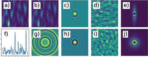
The random phase fluctuations in the incoming beam affect the instantaneous single-particle interference images as shown in Figure 7(b) and 7(g). In the spatial coherence case of Figure 7(b), interference fringes are distorted due to the warped phase of $e_0$. In the temporal coherence case of Figure 7(g), fringes are radially distorted while retaining circular symmetry. This comes from the scattered spherical wavefront which introduces the same temporal delays irrespective of the azymuthal angle.

Due to the rapid fluctuations of the electric field, the instantaneous single-particle interferogram continuously changes from instant to instant and only the average over many statistical realization of the incoming beam is accessible. Here comes the beauty of the self-referencing scheme. Though being hard to grasp by simple visual inspection of Figure 7(b) and 7(g), the instantaneous single-particle interference fringes are basically of two different types. Central fringes are always the interference between the spherical wave generated by a coherence patch (or spike) with the same transmitted coherence patch (or spike). They exhibit small shot-to-shot variations and are reinforced by the averaging process. Contrarily, outermost fringes have no definite phase relations thus they are canceled by the averaging process. The resulting interference pattern is given by

(11) $s_j(\mathbf{x},z)=\frac{2}{kz}\left|\mathrm{\Gamma }\left(\mathbf{x},{\mathbf{x}}_j,t-\frac{z}{c},t-\frac{z}{c}-\frac{|\mathrm{\Delta }{\mathbf{x}}_j{|}^2}{2zc}\right)\right|\cdot |S({\theta }_j)|\cdot cos\left(\frac{k|\mathrm{\Delta }{\mathbf{x}}_j{|}^2}{2z}\right),$(11)

where ${\mathbf{x}}_j$ denotes the position of the $j$-th particle in the scattering plane, $\mathrm{\Delta }{\mathbf{x}}_j=\mathbf{x}-{\mathbf{x}}_j$, ${\theta }_j\sim |\mathrm{\Delta }{\mathbf{x}}_j|/z$ under paraxial conditions and $\mathrm{\Gamma }({\mathbf{x}}_1,{\mathbf{x}}_2,t_1,t_2)=⟨e_0({\mathbf{x}}_1,t_1)e_0^{\ast }({\mathbf{x}}_2,t_2)⟩$ is the Mutual Coherence Function (MCF) describing the spatio-temporal coherence properties of the incoming beam [9–11]. We have also assumed that the scattered wave is phased with the transmitted field. The general case with a finite phase lag is straightforward.

Equation 11(11) $s_j(\mathbf{x},z)=\frac{2}{kz}\left|\mathrm{\Gamma }\left(\mathbf{x},{\mathbf{x}}_j,t-\frac{z}{c},t-\frac{z}{c}-\frac{|\mathrm{\Delta }{\mathbf{x}}_j{|}^2}{2zc}\right)\right|\cdot |S({\theta }_j)|\cdot cos\left(\frac{k|\mathrm{\Delta }{\mathbf{x}}_j{|}^2}{2z}\right),$(11) is valid if the coherence areas propagate as plane wavefronts from the scattering plane to the observation plane. By the same arguments adopted in Section 2.1 [86], this requires $z\ll {\sigma }_{\mathrm{c}\mathrm{o}\mathrm{h}}^2/\lambda$, namely the near field of the coherent portion of the incoming wavefront. Notice the similarity with the coherent case, as also discussed at the end of Section 2.4.1. However, fulfilling the plane wave approximation is now much more crucial. In the coherent case, at larger $z$ it is sufficient to introduce an effective distance, or an effective magnification, to account for the curvature acquired by the coherent wavefront. Conversely, with partially coherent radiation an additional effect comes into play. Adjacent coherence areas mix as they diffract past their near field. Since by definition there is no phase relation between different patches, this eventually cancels any information conveyed by the single-particle interference pattern.

Examples of Equation 11(11) $s_j(\mathbf{x},z)=\frac{2}{kz}\left|\mathrm{\Gamma }\left(\mathbf{x},{\mathbf{x}}_j,t-\frac{z}{c},t-\frac{z}{c}-\frac{|\mathrm{\Delta }{\mathbf{x}}_j{|}^2}{2zc}\right)\right|\cdot |S({\theta }_j)|\cdot cos\left(\frac{k|\mathrm{\Delta }{\mathbf{x}}_j{|}^2}{2z}\right),$(11) are shown in Figure 7(c) and 7(h) for the case of spatial and temporal coherence, respectively. In both cases, circular interference fringes develop as in the coherent case, in spite of the fact that instantaneous fringes are distorted. Their visibility decreases according to the particle form factor and the coherence properties of the incoming beam. Thanks to heterodyne, interference fringes at $\mathbf{x}$ convey the information on the spatio-temporal correlations of the incident field between two points separated by $\mathrm{\Delta }{\mathbf{x}}_j$ and for a delay time $|\mathrm{\Delta }{\mathbf{x}}_j{|}^2/(2zc)$. We can therefore regard the single-particle interference scheme as a continuous two-dimensional wavefront division interferometer and, simultaneously, as a continuous amplitude division interferometer. As a consequence, the single-particle interferogram in Figure 7(c) is elongated along the direction of larger transverse coherence, at variance with Figure 7(h) where the optical path differences are independent on the azymuthal angle.

An equivalent description comes by considering that coherence is the ability of writing stable high-frequency interference fringes [9–11]. We can therefore interpret Equation 11(11) $s_j(\mathbf{x},z)=\frac{2}{kz}\left|\mathrm{\Gamma }\left(\mathbf{x},{\mathbf{x}}_j,t-\frac{z}{c},t-\frac{z}{c}-\frac{|\mathrm{\Delta }{\mathbf{x}}_j{|}^2}{2zc}\right)\right|\cdot |S({\theta }_j)|\cdot cos\left(\frac{k|\mathrm{\Delta }{\mathbf{x}}_j{|}^2}{2z}\right),$(11) as the low-pass filtered hologram of the scattering particle. In this regard, applications to digital holographic microscopy are worth mentioning, where partially coherent illumination effectively suppresses the coherent speckled noise inherent in laser sources, as well as multiple reflection fringes [143–152]. This is definitely an asset for applications such as improved three-dimensional imaging [143], pattern recognition [144], three-dimensional particle flow analysis [146], characterization of deformable objects [147] and studies of vesicle suspensions in shear flow [150], to name a few. Digital holographic microscopy with partially coherent illumination has been originally demonstrated with filtered white LEDs [143]. To cope with the low signals, an intense partially coherent light source has been designed by focusing a laser beam onto a rotating ground glass [145]. Quantitative assessment of noise reduction by theoretical models and experiments has been recently reported [151,152].

3.2. The speckle case: spatial coherence

For the ease of derivation, we consider a sample that scatters light isotropically, thus $S({\theta }_j)\sim S(0)$ in Equation 11(11) $s_j(\mathbf{x},z)=\frac{2}{kz}\left|\mathrm{\Gamma }\left(\mathbf{x},{\mathbf{x}}_j,t-\frac{z}{c},t-\frac{z}{c}-\frac{|\mathrm{\Delta }{\mathbf{x}}_j{|}^2}{2zc}\right)\right|\cdot |S({\theta }_j)|\cdot cos\left(\frac{k|\mathrm{\Delta }{\mathbf{x}}_j{|}^2}{2z}\right),$(11) . Neglecting temporal coherence effects, the MCF reduces to the Mutual Intensity Function (MIF) $J(\mathbf{x},{\mathbf{x}}_j)=⟨e_0(\mathbf{x})e_0^{\ast }({\mathbf{x}}_j)⟩$ describing the spatial coherence properties of the incoming radiation [9–11]. It generally depends on both $\mathbf{x}$ and ${\mathbf{x}}_j$ separately. Here we make the assumption that $J(\mathbf{x},{\mathbf{x}}_j)=J(\mathrm{\Delta }{\mathbf{x}}_j)$. Then, substituting Equation 11(11) $s_j(\mathbf{x},z)=\frac{2}{kz}\left|\mathrm{\Gamma }\left(\mathbf{x},{\mathbf{x}}_j,t-\frac{z}{c},t-\frac{z}{c}-\frac{|\mathrm{\Delta }{\mathbf{x}}_j{|}^2}{2zc}\right)\right|\cdot |S({\theta }_j)|\cdot cos\left(\frac{k|\mathrm{\Delta }{\mathbf{x}}_j{|}^2}{2z}\right),$(11) into Equation 2(2) $i(\mathbf{x},z)=i_0(\mathbf{x})+\sum _{j=1}^{N}2\mathrm{\Re }\{e_t(\mathbf{x},z)e_{s,j}^{\ast }(\mathbf{x},z)\}=i_0(\mathbf{x})+\sum _{j=1}^N{s}_j(\mathbf{x},z),$(2) , the heterodyne signal $2\mathrm{\Re }\{e_0{e}_s^{\ast }\}$ is expressed as a sum of many identical single-particle interferograms, apart from rigid translations. By means of the shift theorem of Fourier Optics [84], the power spectrum of heterodyne speckle reduces to the convolution integral of the radiation MIF with a quadratic phase factor. Under the so-called quasi-stationary phase approximation [153], the convolution integral can be simplified as a simple product. The conditions for the quasi-stationary phase approximation read $z\ll {\sigma }_{\mathrm{c}\mathrm{o}\mathrm{h}}^2/\lambda$, which is automatically fulfilled under the plane-wave approximation. The power spectrum takes the following form, apart from inessential multiplicative factors [32,33,38]:

(12) $I(\mathbf{q},z)={\left|J\left(z\frac{\mathbf{q}}{k}\right)\right|}^{2}T(q,z).$(12)

Equation 12(12) $I(\mathbf{q},z)={\left|J\left(z\frac{\mathbf{q}}{k}\right)\right|}^{2}T(q,z).$(12) shows that the power spectrum of heterodyne speckles exhibits Talbot oscillations enveloped by the squared modulus of the two-dimensional MIF of the incoming radiation, as sketched in Figure 7(d) and 7(e). Furthermore, the relation

(13) $\mathrm{\Delta }\mathbf{x}=z\frac{\mathbf{q}}{k}$(13)

allows to express the radiation MIF as a function of transverse displacements $\mathrm{\Delta }\mathbf{x}$. Equation 13(13) $\mathrm{\Delta }\mathbf{x}=z\frac{\mathbf{q}}{k}$(13) is known as the spatial scaling [32,33,38]. It results from the self-referencing interference between a plane wave and a spherical wavefront, since high-frequency interference fringes are far from the center of the interference pattern. This allows to directly map spatial frequencies $\mathbf{q}$ into lateral displacements $\mathrm{\Delta }\mathbf{x}$. It is an example of the well-known concept of local spatial frequencies in Fourier Optics [84].

Equation 13(13) $\mathrm{\Delta }\mathbf{x}=z\frac{\mathbf{q}}{k}$(13) shows that, in principle, larger distances are required to properly probe larger coherence areas. Furthermore, since the radiation MIF is measured at the plane of the particles, measurements at different $z$ must give the same result. 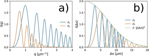The envelopes of the Talbot oscillations indeed fit a unique master curve upon the spatial scaling, in spite of the fact the raw power spectra $I(\mathbf{q},z)$ describe different curves. This effect, which we refer to as the spatial master curve criterion [32,33,38], is depicted in Figure 8.

Figure 8. (a) Simulated power spectra with partially spatially coherent radiation for two different sample-detector distances. (b) The envelopes of the Talbot oscillations fit a unique master curve upon the spatial scaling

An interesting interpretation of the spatial scaling comes by considering that, at a given $\mathrm{\Delta }\mathbf{x}=z\mathbf{q}/k$, data oscillate due to the contributions from different $z$. Maxima of these oscillations describe the radiation MIF. This is entirely equivalent to the method adopted by Pfeiffer et al. [154] with a shearing grating interferometer to extract the visibility curves of partially coherent X-ray radiation.

By recalling the Wiener-Khinchin theorem [9–11], the autocorrelation function of heterodyne speckles takes the following form under the quasi-stationary phase approximation:

(14) $ACF(\mathrm{\Delta }\mathbf{x},z)=\left\{\int {\left|J\left(z\frac{\mathbf{q}}{k}\right)\right|}^2{e}^{-i\mathbf{q}\cdot \mathrm{\Delta }\mathbf{x}}\mathrm{d}\mathbf{q}\right\}-\left\{\frac{k\pi }{z}{\left|J\left(\frac{\mathrm{\Delta }\mathbf{x}}{2}\right)\right|}^{2}sin\left[\frac{k|\mathrm{\Delta }\mathbf{x}{|}^2}{4z}\right]\right\}.$(14)

The first term in Equation 14(14) $ACF(\mathrm{\Delta }\mathbf{x},z)=\left\{\int {\left|J\left(z\frac{\mathbf{q}}{k}\right)\right|}^2{e}^{-i\mathbf{q}\cdot \mathrm{\Delta }\mathbf{x}}\mathrm{d}\mathbf{q}\right\}-\left\{\frac{k\pi }{z}{\left|J\left(\frac{\mathrm{\Delta }\mathbf{x}}{2}\right)\right|}^{2}sin\left[\frac{k|\mathrm{\Delta }\mathbf{x}{|}^2}{4z}\right]\right\}.$(14) describes the effects of partial spatial coherence on the size and shape of Heterodyne Near Field Speckles, as shown in Figure 7(d). By Fourier Optics argument, it has a characteristic width given by

(15) $d_{\mathrm{s}\mathrm{p},\mathrm{s}\mathrm{p}\mathrm{a}\mathrm{t}}=\frac{\lambda z}{{\sigma }_{\mathrm{c}\mathrm{o}\mathrm{h}}}.$(15)

The second term in Equation 14(14) $ACF(\mathrm{\Delta }\mathbf{x},z)=\left\{\int {\left|J\left(z\frac{\mathbf{q}}{k}\right)\right|}^2{e}^{-i\mathbf{q}\cdot \mathrm{\Delta }\mathbf{x}}\mathrm{d}\mathbf{q}\right\}-\left\{\frac{k\pi }{z}{\left|J\left(\frac{\mathrm{\Delta }\mathbf{x}}{2}\right)\right|}^{2}sin\left[\frac{k|\mathrm{\Delta }\mathbf{x}{|}^2}{4z}\right]\right\}.$(14) stems from the Talbot oscillations in the power spectrum of heterodyne speckles. It therefore vanishes in presence of the walkoff effect or for 3D scattering (see Sections 2.3.1 and 2.3.2).

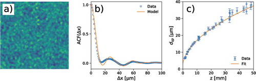
An example of self-referencing speckles for the case of partial spatial coherence is reported in Figure 9(a). Speckles are generated by a filtered white LED with the setup described in [28,29]. The corresponding autocorrelation function is plotted in Figure 9(b), where the expected curve based on Equation 14(14) $ACF(\mathrm{\Delta }\mathbf{x},z)=\left\{\int {\left|J\left(z\frac{\mathbf{q}}{k}\right)\right|}^2{e}^{-i\mathbf{q}\cdot \mathrm{\Delta }\mathbf{x}}\mathrm{d}\mathbf{q}\right\}-\left\{\frac{k\pi }{z}{\left|J\left(\frac{\mathrm{\Delta }\mathbf{x}}{2}\right)\right|}^{2}sin\left[\frac{k|\mathrm{\Delta }\mathbf{x}{|}^2}{4z}\right]\right\}.$(14) is also shown for comparison. Oscillations at larger $\mathrm{\Delta }x$ stem from the Talbot oscillations in the corresponding power spectrum, as discussed above. The measured speckle size as a function of the sample-detector distance is reported in Figure 9(c). The linear behavior at larger $z$ is in agreement with Equation 15(15) $d_{\mathrm{s}\mathrm{p},\mathrm{s}\mathrm{p}\mathrm{a}\mathrm{t}}=\frac{\lambda z}{{\sigma }_{\mathrm{c}\mathrm{o}\mathrm{h}}}.$(15) .

Figure 9. (a) Heterodyne Near Field Speckles, (b) radial profile of the corresponding autocorrelation functions and (c) speckle size as a function of the sample-detector distance for the case of limited spatial coherence. Plots (a) and (b) refer to z = 5 mm. The expected curve based on Equation 14 is also reported for comparison in (b). The fitted curve in (c) is obtained from Equation 15 by also including the effects from the finite size of the scatterers

Equation 12(12) $I(\mathbf{q},z)={\left|J\left(z\frac{\mathbf{q}}{k}\right)\right|}^{2}T(q,z).$(12) is generalized as follows to include the effects of the particle form factor $S(\mathbf{q})$ and the response of the optical system $H(\mathbf{q})$:

(16) $I(\mathbf{q},z)=S(\mathbf{q}){\left|J\left(z\frac{\mathbf{q}}{k}\right)\right|}^{2}T(q,z)H(\mathbf{q}).$(16)

Equation 16(16) $I(\mathbf{q},z)=S(\mathbf{q}){\left|J\left(z\frac{\mathbf{q}}{k}\right)\right|}^{2}T(q,z)H(\mathbf{q}).$(16) is quite common in the X-ray domain, where it is the square of the field relation used in X-ray phase-contrast imaging [116–118,155,156] and X-ray Talbot interferometry [154,157–163]. It is also well known in TEM imaging [92,138], where it describes electron scattering by amorphous films. In the TEM context, the product $J\cdot T\cdot H$ is referred to as the effective transfer function, whereas $J$ and $H$ are called envelope damping functions. Equation 16(16) $I(\mathbf{q},z)=S(\mathbf{q}){\left|J\left(z\frac{\mathbf{q}}{k}\right)\right|}^{2}T(q,z)H(\mathbf{q}).$(16) basically states that resolution in direct space is limited by the spatial coherence of the source and the quality of the relay optics.

3.3. The speckle case: temporal coherence

Neglecting spatial coherence effects, the MCF reduces to the Self Coherence Function (SCF) $\mathrm{\Gamma }(t_1,t_2)=⟨e_0(t_1)e_0^{\ast }(t_2)⟩$ describing the temporal coherence properties of the incoming radiation [9–11]. Similarly to the spatial coherence case, we make the assumption that $\mathrm{\Gamma }(t_1,t_2)=\mathrm{\Gamma }(t_1-t_2)$. At variance with the spatial coherence case, however, it is worth noting how the heterodyne signal $2\mathrm{\Re }\{e_0{e}_s^{\ast }\}$ already involves many identical contributions. Dropping inessential multiplicative factors, under the quasi-stationary phase approximation [153] the power spectrum of heterodyne speckles takes the form [28,38]

(17) $I(\mathbf{q},z)={\left|\mathrm{\Gamma }\left(\frac{z{q}^2}{2k^{2}c}\right)\right|}^{2}T(q,z).$(17)

The quasi-stationary phase approximation for the temporal coherence case reads $l_{\mathrm{c}\mathrm{o}\mathrm{h}}\gg \lambda /2$, which is always fulfilled for standard light sources. The plane-wave approximation still requires to operate the technique in the near field of the coherence areas.

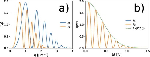
Notice how the power spectrum for the temporal coherence is circularly symmetric, as shown in Figure 7(i) and 7(j), whereas the power spectrum for the spatial coherence is elongated along the direction of larger coherence. In both cases, the power spectrum of heterodyne speckles echoes the single-particle fringe visibility, as it can be seen by comparing Figure 7(e) with Figure 7(c), and Figure 7(j) with Figure 7(h). Indeed, a remarkable aspect of the self-referencing layout lies in the fact that, when moving from a single particle to speckles, the information about the visibility of a certain fringe is transferred into the amplitude of a certain spatial frequency. The correspondence between fringes and spatial frequencies is made quantitative by the spatial scaling of Equation 13(13) $\mathrm{\Delta }\mathbf{x}=z\frac{\mathbf{q}}{k}$(13) for transverse coherence, and by the following temporal scaling for temporal coherence [28,38]:

(18) $\mathrm{\Delta }t=\frac{z{q}^2}{2k^{2}c}.$(18)

Equation 18(18) $\mathrm{\Delta }t=\frac{z{q}^2}{2k^{2}c}.$(18) maps Fourier wave vectors into temporal delays, allowing to measure the SCF of the incident beam from the envelope of Talbot oscillations. As for the spatial scaling, it comes from the spatial frequency localization, since outermost fringes with high spatial frequencies are generated by larger delays of the spherical wave with respect to the plane wavefront of the coherence areas. Notice that the square law of Equation 18(18) $\mathrm{\Delta }t=\frac{z{q}^2}{2k^{2}c}.$(18) is a direct consequence of the spherical wavefront of the scattered wave. Upon the temporal scaling, the envelopes of the Talbot oscillations fit a unique master curve, while the Talbot oscillations themselves overlap. We refer to this peculiar feature as the temporal master curve criterion [38], and an example based on simulations is reported in Figure 10.

Figure 10. (a) Simulated power spectra with partially temporally coherent radiation for two different sample- detector distances. (b) The envelopes of the Talbot oscillations fit a unique master curve upon the temporal scaling. Notice how Talbot oscillations actually overlap in this case, at variance with Figure 8

The autocorrelation function of heterodyne speckles with partial temporal coherence exhibits similar features to the spatial coherence case:

(19) $ACF(\mathrm{\Delta }\mathbf{x},z)=\left\{\int {\left|\mathrm{\Gamma }\left(\frac{z{q}^2}{2k^{2}c}\right)\right|}^2{e}^{-i\mathbf{q}\cdot \mathrm{\Delta }\mathbf{x}}\mathrm{d}\mathbf{q}\right\}-\left\{\frac{k\pi }{z}{\left|\mathrm{\Gamma }\left(\frac{|\mathrm{\Delta }\mathbf{x}{|}^2}{8cz}\right)\right|}^{2}sin\left[\frac{k|\mathrm{\Delta }\mathbf{x}{|}^2}{4z}\right]\right\}.$(19)

In particular, the first term in Equation 19(19) $ACF(\mathrm{\Delta }\mathbf{x},z)=\left\{\int {\left|\mathrm{\Gamma }\left(\frac{z{q}^2}{2k^{2}c}\right)\right|}^2{e}^{-i\mathbf{q}\cdot \mathrm{\Delta }\mathbf{x}}\mathrm{d}\mathbf{q}\right\}-\left\{\frac{k\pi }{z}{\left|\mathrm{\Gamma }\left(\frac{|\mathrm{\Delta }\mathbf{x}{|}^2}{8cz}\right)\right|}^{2}sin\left[\frac{k|\mathrm{\Delta }\mathbf{x}{|}^2}{4z}\right]\right\}.$(19) describes the size and shape of heterodyne speckles under partially temporally coherent light. Opposite to the spatial coherence case, speckles are isotropic as shown in Figure 7(i) and they have a characteristic width given by

(20) $d_{\mathrm{s}\mathrm{p},\mathrm{t}\mathrm{e}\mathrm{m}\mathrm{p}}=\sqrt{\frac{{\lambda }^{2}z}{2c{\tau }_{\mathrm{c}\mathrm{o}\mathrm{h}}}}=\sqrt{\frac{{\lambda }^{2}z}{2l_{\mathrm{c}\mathrm{o}\mathrm{h}}}}.$(20)

An example of self-referencing speckles for the case of partial temporal coherence is reported in Figure 11(a), and the corresponding autocorrelation function is plotted in Figure 11(b) alongside with the expected curve given by Equation 19(19) $ACF(\mathrm{\Delta }\mathbf{x},z)=\left\{\int {\left|\mathrm{\Gamma }\left(\frac{z{q}^2}{2k^{2}c}\right)\right|}^2{e}^{-i\mathbf{q}\cdot \mathrm{\Delta }\mathbf{x}}\mathrm{d}\mathbf{q}\right\}-\left\{\frac{k\pi }{z}{\left|\mathrm{\Gamma }\left(\frac{|\mathrm{\Delta }\mathbf{x}{|}^2}{8cz}\right)\right|}^{2}sin\left[\frac{k|\mathrm{\Delta }\mathbf{x}{|}^2}{4z}\right]\right\}.$(19) . The same setup of Figure 9 has been used, but with the band-pass filter removed. Notice how the speckles become larger as the coherence properties are reduced. The measured speckle size as a function of the sample-detector distance exhibits the expected power-law behavior from Equation 20(20) $d_{\mathrm{s}\mathrm{p},\mathrm{t}\mathrm{e}\mathrm{m}\mathrm{p}}=\sqrt{\frac{{\lambda }^{2}z}{2c{\tau }_{\mathrm{c}\mathrm{o}\mathrm{h}}}}=\sqrt{\frac{{\lambda }^{2}z}{2l_{\mathrm{c}\mathrm{o}\mathrm{h}}}}.$(20) , as shown in Figure 11(c).

Figure 11. (a) Heterodyne Near Field Speckles, (b) radial profile of the corresponding autocorrelation functions and (c) speckle size as a function of the sample-detector distance for the case of limited temporal coherence. Plots (a) and (b) refer to the same z = 5 mm as in Figure 9. Notice how speckles become larger as the coherence properties are reduced. The expected curve based on Equation 19 is also reported for comparison in (b). The fitted curve in (c) is obtained from Equation 20 by also including the effects from the finite size of the scatterers

4. X-ray Heterodyne Near Field Speckles

The interaction of X-rays with matter is described in terms of the complex refractive index $n=1-\delta +i\beta$. Here $\delta$ is responsible for phase shifts in the incoming beam due to elastic scattering, while $\beta$ gives rise to absorption due to the photoelectric effect and inelastic Compton scattering. For most light materials in the hard X-ray region of the spectrum, and away from absorption edges, both $\delta$ and $\beta$ are significantly smaller than unity, with $\delta \sim {10}^{-5}÷{10}^{-6}$ being typically three orders of magnitude larger than $\beta \sim {10}^{-8}÷{10}^{-9}$ . This accounts for the fact that X-ray phase-contrast imaging yields superior results with respect to conventional X-ray absorption imaging.

Owing to the low interaction of X-rays with matter, heterodyne conditions are easily fulfilled. Most samples behave as weakly-interacting phase objects [164] that generate a weak scattered field while simultaneously letting the intense incident beam pass. With random media, this naturally leads to the formation of heterodyne speckles. We have discussed similar conditions for the TEM in Section 2.4.5.

As far as spatial coherence is concerned, X-rays from third-generation synchrotron light sources are more similar to standard light sources such as bulbs and LEDs than to a laser. Therefore the formalism of Section 3 applies. One of the advantages of operating Heterodyne Near Field Speckles with X-rays is that the near field regime extends to distances as large as 1 m for a modest transverse coherence length of 10 $\mu$m at a photon energy of 12 keV ($\lambda =0.1$ nm), thus making the experimental layout more flexible. However, the short wavelength also implies that the Talbot transfer function is sensibly different from unity in the entire $q$ range. Thus, the Talbot effect generally plays an important role with X-ray radiation. By contrast, the Talbot transfer function is easily made flat in the visible range [15,17].

4.1. Static and dynamic X-ray scattering measurements

Applications to static and dynamic X-ray scattering studies have been described in the original work by Cerbino et al. [30], followed a few years later by the analysis by Lu et al. [31].

In the first work by Cerbino et al. [30], the authors show how to obtain absolute static and dynamic scattering data in spite of the limited transverse coherence of X-ray synchrotron radiation. As for the fully coherent case, it is only required that the Fourier components of the scattered field interfering with the reference beam be determined solely by the angular distribution of the scattered light. This implies that the edge of the coherence patches is not sensed and the deep near field conditions accordingly read as $z\ll {\sigma }_{\mathrm{c}\mathrm{o}\mathrm{h}}d/\lambda$. Notice how this condition can be considered as a generalization of Equation 5(5) $z\ll \frac{Dd}{\lambda },$(5) by taking $D$ as the diameter of the coherent portion of the incoming wavefront (also refer to the discussion at the end of Section 2.4.1). Whilst being much more stringent than the near field of the coherence areas, the deep near field conditions allow to neglect $|J{|}^2$ in Equation 16(16) $I(\mathbf{q},z)=S(\mathbf{q}){\left|J\left(z\frac{\mathbf{q}}{k}\right)\right|}^{2}T(q,z)H(\mathbf{q}).$(16) . Furthermore, both the plane-wave approximation and the quasi-stationary phase approximation hold.

Absolute static scattering data have been reported for a static cellulose acetate membrane with nominal pore size 0.45 $\mu$m [30] and for a colloidal suspension of polystyrene spheres 4 $\mu$m in diameter [31]. For the case of the static membrane, measurements with the speckle method at previously inaccessible wave vectors evidenced a peak in the form factor due to the quasi-spinodal structure of alternating voids typical of membranes [165].

Similarly to the cases discussed in Section 2.4.2, analysis of the intermediate scattering function allows to extract low-angle dynamic scattering data. For small particles undergoing pure Brownian motions, agreement is found with conventional far-field X-ray Photon Correlation Spectroscopy data and with theoretical predictions. For larger particles, shorter relaxation times are measured since sedimentation leads to denser samples with faster dynamics [31]. At higher volume fractions, multiple scattering is evidenced from the faster relaxation times and the tapering induced on Talbot oscillations [31]. Similar effects had already been reported in the optical domain [120]. Recently, a theoretical model has been proposed to quantitatively assess the effects of multiple scattering on the technique [23].

Reference [30] also provides the first X-ray Heterodyne Near Field Speckle measurements of the uneven frequency response of scintillators typically used for the detection of X-ray photons (the term $H$ in Equation 16)(16) $I(\mathbf{q},z)=S(\mathbf{q}){\left|J\left(z\frac{\mathbf{q}}{k}\right)\right|}^{2}T(q,z)H(\mathbf{q}).$(16) . Further contributions generally arise from the relay optics, as thoroughly discussed in [31]. The speckle method allows to accurately characterize the response of the system by taking advantage of the uniform scattering from small samples, without changing the experimental setup. This is entirely equivalent to feed the system with white noise as commonly done in electronics. It is only required to perform measurements close enough to the scattering sample, where $J\sim 1$ in Equation 16(16) $I(\mathbf{q},z)=S(\mathbf{q}){\left|J\left(z\frac{\mathbf{q}}{k}\right)\right|}^{2}T(q,z)H(\mathbf{q}).$(16) for $z\mathbf{q}/k\to 0$ [30–32,35].

4.2. Coherence characterization and beam size diagnostics

In ref. [30], it is discussed how the effects of partial coherence become relevant at larger detector distances. The shorter horizontal coherence length is first sensed, far field conditions set in and the speckle size increases along the horizontal direction [142]. The effect is particularly evident for undulator X-ray beams due to the much larger vertical coherence length [39,40]. Analogous observations in the optical domain with strongly astigmatic laser beams [24] prove that the near field is intimately related to the illumination conditions, as discussed at the end of Section 2.4.1.

The first measurements of transverse coherence with X-ray Heterodyne Near Field Speckles have been reported by Alaimo et al. [32] and Manfredda [166]. By means of an imaging geometry, the 2D transverse coherence of the X-ray beam from an undulator was probed at the source position. In particular, the size of the coherence patches in the vertical direction is close to the source size, implying that the strongly elongated undulator source is almost coherent in the vertical direction. Despite the optical aberrations introduced by the focusing optics, the transverse coherence length is preserved thanks to the fully-developed circular Gaussian statistics of the coherence patches [9–11].

The method has then been applied to characterize the two dimensional transverse coherence of a SASE FEL [33], a typical case where the transverse coherence length is comparable to the photon beam size and, additionally, the radiation footprint exhibits a high shot-to-shot variability. Single-shot performances of the technique are achieved by high-pass filtering each individual image. Measurements were performed with the sensor collecting the entire radiation wavefront in order to evaluate the beam autocorrelation function. The latter provides the proper normalization to the measured power spectra of heterodyne speckles to account for the stochastic intensity changes across the beam [33]. In other approaches, the transverse coherence of FEL radiation is measured from the properties of homodyne speckles [167–169], which however prevent to access the beam intensity autocorrelation function. The heterodyne speckle approach allows to directly estimate the number of transverse modes in the radiation beam from the simultaneous measurements of the beam width and the transverse coherence length. The number of longitudinal modes can then be retrieved from the first order statistics of the beam intensity fluctuations [33,167–169].

Recently [35], coherence measurements with Heterodyne Near Field Speckles have been extended to the radiation emitted by a bending dipole with lower bandwidth requirements of $\mathrm{\Delta }E/E\sim {10}^{-2}$ compared with the typical value of $\mathrm{\Delta }E/E\sim {10}^{-4}$ of undulator beamlines. At variance with the original layout [32], measurements were performed at a single distance by raster scanning a phase membrane. The measured power spectrum is then fitted to Equation 16(16) $I(\mathbf{q},z)=S(\mathbf{q}){\left|J\left(z\frac{\mathbf{q}}{k}\right)\right|}^{2}T(q,z)H(\mathbf{q}).$(16) by assuming a Gaussian coherence factor. The method was tested under different coherence conditions and results were in agreement with independent grating-based measurements [154]. While the Gaussian assumption certainly holds for the synchrotron radiation from a bending dipole, it fails to describe the transverse coherence of undulator X-ray beams, especially for next-generation, nearly diffraction-limited sources [170,171]. In this view, we stress how the Heterodyne Near Field Speckle technique is intrinsically model independent and additional information can be gauged from the measured curves, as shown by Alaimo et al. [30].

The main recent advances of coherence measurements with the Heterodyne Near Field Speckle technique concern the characterization of temporal coherence of broadband synchrotron radiation [37,38] and applications to particle beam diagnostics [39,40].

The first Heterodyne Near Field Speckle measurements of temporal coherence of synchrotron radiation have been reported by Siano et al. [38] for the visible light emitted by a bending dipole. The authors show how the temporal coherence of the emitted synchrotron radiation is probed in the actual operating conditions of the beamline. In particular, besides conveying the information on the single particle spectrum, measurements are affected by beamline characteristics as well as by experimentally-related parameters, mainly the spectral response of the sample, the CCD sensor, the band-pass filters. Since these contributions are known, they can be modeled as a single effective band-pass filter acting on the incoming radiation spectrum. This allows to introduce a spectral calibration function to characterize the beamline performances alone [38].

The possibility offered by Heterodyne Near Field Speckles of accessing the 2D transverse coherence of a light source [32,33,35] is of great interest to the accelerator community for non-invasive, 2D transverse beam profile diagnostics. The technique has been developed during the last years at an undulator beamline [39]. The first experimental results from a proof of principle test by changing the beam coupling of the storage ring have been recently reported [40]. Free-space propagation conditions were obtained by removing slits and focusing elements to avoid degradation of the coherence properties by optical components along the beamline. Discrepancies arising along the vertical direction with respect to the predictions based on the Van Cittert and Zernike theorem [40] prove that the radiation source cannot be modeled as quasi-homogeneous [170,171]. Complete simulations based on the refurbished Fourier-Optics-based theory as proposed by Geloni et al. [170], extended to include higher undulator harmonics and the finite energy spread of the electron beam [172], match with preliminary results within the experimental uncertainties. This confirms that the Van Cittert and Zernike theorem fails in presence of small emittances. It is here important to notice how similar conclusions from earlier experiments on a nearly diffraction-limited undulator source have been reported independently [173].

4.3. X-ray wavefront sensing and X-ray optics metrology

Heterodyne Near Field Speckles also provide a very efficient approach to quantitatively characterize the wavefront of a partially coherent X-ray beam. The technique is known as X-ray Speckle Tracking (XST) [41,56] and it provides the 2D phase gradient of the wavefront with the same or higher accuracy compared to state-of-the-art grating-based instruments or Hartmann sensors.

The X-ray beam falling onto a static diffuser as a piece of abrasive paper [56] or a random phase membrane [41] generates stochastic speckles. In deep near field conditions, the speckle size is controlled by the size of the scatterers [113,114]. Distortions in the speckle pattern are caused only by phase changes in the incoming beam. In particular, speckles are laterally displaced according to the local phase gradient of the wavefront, therefore acting as high-frequency markers for sensing the beam phase. By tracking the distortions between similar speckle signals, the differential phase of the incoming wavefront is obtained from the trajectory of the corresponding geometrical rays.

In an absolute configuration, two speckle images are taken at two different distances from the scattering sample. This allows to characterize the incident wavefront including the effects of all optical elements upstream of the diffuser. It is therefore suitable for quantitative wavefront sensing (absolute metrology) [41–44]. This configuration is also adopted to optimize adaptive optics for beam shaping [45,48–52], since the wavefront from a whole series of optical components is of interest. At variance, a differential configuration is used to perform in-line at-wavelength metrology of individual optical elements [46,47,53]. The two speckle images are acquired at the same distance from the scattering sample. The first image acts as a reference and it is obtained with the optical element out from the beam. The second image is obtained with the optics inserted along the beam path.

The tracking of speckle displacements is performed on small sub-regions (windows) by cross-correlating the two acquired frames [41,56,57] or by least square minimization with respect to a physical model [60]. It can be shown that such recipes are indeed equivalent [54]. In both cases, a larger window results in higher accuracy, though at the expense of spatial resolution. The method takes inspiration from mechanics and particle image velocimetry, where such correlation algorithms are extensively adopted to infer mechanical deformations and fluid flows. It is also worth noting the strong similarity arising with HSV [25–27], where changes in the speckle pattern mirror the movement of the particles and the the cross-correlation analysis yields information on the tracer trajectories. In the XST technique, speckle changes arise from wavefront distortions and the cross-correlation analysis allows to retrieve the trajectory of the beam rays.

The main drawback of the XST implementation stems from the poor spatial resolution since the analysis window must be necessarily larger than the speckle size. To overcome such limitation, different acquisition schemes and data analysis procedures have been conceived, based on 2D and 1D scans [57,74]. In X-ray Speckle Scanning (XSS), the two data sets are generated by scanning the scatterer using a fine 2D mesh. The cross-correlation is then computed pixel-wise for different positions of the speckle generator. In this regard, the technique can be considered as a generalized version, to a random intensity modulation, of X-ray grating interferometry in the phase-stepping mode [59,68]. The sensitivity is directly proportional to the mesh step, which is typically in the range of the pixel size or smaller. Combined with the pixel-wise analysis, this enables a much higher resolution compared to XST. In XSS-1D, the two data sets come from a 1D scan combined with an asymmetric analysis window [72]. This scheme is equivalent to XSS in the direction of the scan and to XST in the orthogonal direction. In XSS self-correlation mode [52], a single scan of the speckle generator is performed, either 1D or 2D. The cross-correlation is computed between nearby pixels for different scatterer positions. Indeed, different pixels in the detector plane measure the same signals for different positions of the diffuser. It can be shown that the local wavefront curvature is directly accessed from such delayed, or shear, signals [57]. The XSS self-correlation mode is exploited to characterize strongly focusing optics and systems that are projected along the orthogonal directions, e.g. Kirkpatrick-Baez mirrors. It is interesting to note how the principles of the technique are equivalent to those of the Asymmetric Lateral Coherence, a novel scanning interferometric technique originally introduced for coherence measurements of laser-driven and undulator-based sources [174–176] and recently extended to wavefront sensing in the visible range [177]. By properly scanning an array of double-slits with different spacings, the shear displacement of a reference fringe allows to measure the Laplacian of the phase distribution, namely the wavefront curvature [177]. By further exploiting the peculiar intrinsic curvature properties of vortex beams, the method has recently succeeded in providing a strictly local measurement of the topological charge in single-shot conditions [178–182]. The analogy with the XSS self-correlation mode can be made explicit by the correspondence between the double-slit scan with the shear displacement of the reference fringe and the diffuser scan with the shear of the maximum of the cross-correlation function.

Recently, the X-ray Speckle Vector Tracking (XSVT) [71,76] and the Unified Modulated Pattern Analysis (UMPA) [78] approaches have been proposed to further reduce the number of acquired speckle images. In XSVT, two data sets of $N$ images are acquired at different positions of the speckle generator. The redundant information coming from different image couples gives higher sensitivity with respect to XST. In the original work, XSVT was proposed with a unitary window to perform pixel-wise analysis. To increase the accuracy and to reduce the number of acquired images, later implementations have introduced small analysis windows at the cost of spatial resolution, thus realizing an hybrid XST-XSVT [76]. In this latter case, if the data processing is based on least-square minimization rather than on cross-correlations, the technique is commonly referred to as UMPA [53,78]. It has been shown to be applicable also to periodic patterns such as the Talbot self-images by a phase grating [53,78].

Metrology demands for high sensitivity and quantitative accuracy, and scan time is generally not an issue. XST has the lowest spatial resolution among the aforementioned methods, determined by the size of the analysis window and ultimately limited by the speckle size. Nonetheless, it allows to perform single pulse wavefront metrology [42], with potential applications at FELs [44] where the beam properties vary shot-by-shot. To this aim, an absolute configuration should be adopted where the two speckle images are acquired simultaneously by two subsequent detectors, the first one being a semitransparent screen [42]. XSVT provides a resolution ultimately limited by the detector, while XST-XSVT and UMPA have a lower resolution due to the finite analysis window, though still higher with respect to XST. Although XSS is the slowest implementation, it provides the highest angular sensitivity. It has been reported that the angular sensitivity of XST, XSVT, XST-XSVT and UMPA is directly proportional to the effective pixel size, while it is proportional to the diffuser step size for XSS [79]. In any case, to achieve accuracy on the wavefront gradient of a few nanoradians, nano-positioners are required [43,49,51].

The method has found huge applications at synchrotron radiation facilities, for the characterization of the wavefront curvature [41], aberrations and beam astigmatism [52]. By tracking a large pixel subset, horizontal and vertical beam drifts and tilts can be followed [52], with straightforward applications to beamline design and optimization. Inline mirror metrology has also been demonstrated [45,47–51,53]. The methods can also be used for adaptive optics optimization, with potential applications to beam focusing and shaping and to reduce optical aberrations [45,48]. As an example, optimization of the optics to generate top-hat beams with uniform intensity profiles is important to reduce radiation damage in specimen [49]. Further results relate to the determination of mirror slope errors and mirror alignment with a nanoradian accuracy [43,49,51]. Weakly refractive optics such as 2D compound refractive lenses [46] and 1D parabolic lenses made from berillium or polymer materials [53] have been characterized. Recently, the principles of the XST technique have also been successfully extended to the visible range [183].

The key of the technique stems from the near field conditions. Similarly to the HSV technique [25–27], they allow to introduce a one-to-one mapping between speckles and portions of the wavefront. Notice how the technique is not limited to the deep near field regime, but can be operated within the near field of the coherence areas [41]. In this case, the speckle size may be influenced by the transverse coherence length of the X-ray beam (see Section 3). Furthermore, in the absolute configuration, the two data sets should be acquired at a longitudinal distance not exceeding $d_{sp}^2/\lambda$, namely the length of individual speckles as predicted by Fourier Optics [184,185].

4.4. X-ray imaging

The same schemes and data processing algorithms can also be implemented for efficient phase-contrast imaging. By tracking the lateral displacements of X-ray Heterodyne Near Field Speckles induced by a phase object, the decrement $\delta$ of the real part of refractive index can be determined [56].

In addition, multimodal imaging is possible [57,63,72]. Indeed, when a sample intercepts the X-ray beam, it modulates the speckle pattern in three ways: i) speckles are displaced due to refraction in the specimen, ii) their mean intensity changes due to absorption and iii) the visibility of the speckle pattern is reduced due to small-angle scattering by unresolved features such as cracks and nanopores. The overall reduction in intensity allows to obtain absorption maps of the object under investigation, hence the imaginary part $\beta$ of the refractive index of the sample. The reduction in speckle contrast allows to gauge the so-called dark-field images of the sample [60,64,70,77], which deliver valuable complementary information on the small-scale structures.

The principles of multimodal imaging apply to other imaging techniques as well, especially to X-ray grating interferometry [75]. Indeed, it has been shown both theoretically and experimentally how grating-based imaging in phase-stepping modality can be considered as a special case of scanning speckle-based imaging [59,68]. Compared to the grating-based approach, speckle-based imaging does not suffer from the phase wrapping limitation arising with periodic interference patterns, and it does not require precise alignments. The position of the observation plane is not limited to the fractional Talbot distances as in grating-based layouts and it can lie anywhere within the near field conditions. Speckle-based imaging also allows to extract two orthogonal phase gradients even for 1D scans, since speckles are inherently 2D. It is customarily accepted that speckle-based imaging can be advantageously operated over grating-based imaging at synchrotron light sources, while the opposite holds for laboratory-based X-ray sources. In this regard, the two methods are expected to be complementary in their applications.

Opposite to metrology and wavefront sensing, the context of phase imaging typically demands for the lowest number of acquisitions, especially with biological samples. The XST implementation of the technique is therefore particularly suitable to this aim being highly dose efficient [80,82], though intrinsically endowed with poor spatial resolutions. The XSS scheme can be implemented for high-resolution applications, and XSS-1D also provides high acquisition speeds. The hybrid XST-XSVT and recently introduced UMPA approaches [78] significantly reduce the number of acquired frames. In these cases, the analysis window is typically a few pixels wide, providing good resolutions. Furthermore, the number of acquired frame and the width of the analysis windows are typically correlated, thus making these approaches highly tailored for specific needs [74].

The first demonstrations of speckle-based phase-contrast imaging were reported at synchrotron radiation facilities [56–59]. Nonetheless, the low requirements on spatial and temporal coherence make speckle-based multimodal imaging appealing for laboratory sources as well [60]. Transmission, differential phase and dark-field images have indeed been obtained for several samples with polychromatic, low-brilliance X-ray sources [60,62,81].

By combining speckle-based multimodal imaging with tomographic reconstruction algorithms, 3D volume rendering of samples can be achieved [65]. The complementary 3D absorption, phase-contrast and dark-field information allow to retrieve the 3D distribution of the complex refractive index of the specimen, as well as its 3D scattering properties [66]. Qualitative as well as quantitative transmission and phase-contrast tomography has been demonstrated [65,66,71,76].

With polychromatic X-rays, the beam hardening effects should be taken into account for quantitative assessment of the optical properties of a specimen [60]. This effect, arising from the propagation of broadband X-rays through the sample, is somewhat similar to the spectral calibration function discussed in Section 4.2. Beam hardening artifacts have also been extensively investigated by numerical simulations [67,69]. It is also shown that, in the ideal case of monochromatic X-rays, the speckle contrast is modulated according to the Talbot transfer function of the heterodyne regime. Recently, the influence of the diffuser grain size on the speckle-based imaging techniques has been numerically investigated [83]. It has been demonstrated that smaller grain sizes are required to achieve higher resolutions, since they preserve the high-frequency information thanks to a broader form factor, in agreement with Equation 16(16) $I(\mathbf{q},z)=S(\mathbf{q}){\left|J\left(z\frac{\mathbf{q}}{k}\right)\right|}^{2}T(q,z)H(\mathbf{q}).$(16) .

For a more complete description of the X-ray speckle-based techniques, with rigorous mathematical derivations and practical examples, the recent reviews by Zdora [79] and Berujon et al. [54,55] are highly recommended.

5. Unified Fourier Optics approach to Heterodyne Near Field Speckles

Heterodyne Near Field Speckles in both coherent and partially coherent light arise from the superposition of many independent single-particle contributions, as shown in Section 2.1, 3.2 and 3.3. Generalizing the discussion at the end of Section 3.1, each single-particle interference image can be regarded as the low-pass filtered hologram of a spherical wave. This implies that the space-bandwidth product of the intensity distribution is limited and speckles with a finite size arise because higher spatial frequencies are suppressed. In terms of Fourier Optics, the angular spectrum of the scattered plane waves interfering with the trans-illuminating beam in the self-referencing geometry is therefore limited. Setting the Talbot oscillations issue aside, the power spectrum of heterodyne speckles takes the general form $I(\mathbf{q},z)=\tilde{S}(\mathbf{q},z)$, where $\tilde{S}(\mathbf{q},z)=4S(\mathbf{q})$ in Section 2.2, $\tilde{S}(\mathbf{q},z)=|J(z\mathbf{q}/k){|}^2$ in Section 3.2 and $\tilde{S}(\mathbf{q},z)=|\mathrm{\Gamma }(z{q}^2/(2k^{2}c)){|}^2$ in Section 3.3. Accordingly, $\tilde{S}$ extends up to a characteristic wave vector $q_{\mathrm{m}\mathrm{a}\mathrm{x}}=k{\theta }_{\mathrm{m}\mathrm{a}\mathrm{x}}$, where ${\theta }_{\mathrm{m}\mathrm{a}\mathrm{x}}$ is the most limiting angle among the following:

i) the scattering angle of the particles $\lambda /d$;

ii) the angle subtended by the coherence areas ${\sigma }_{\mathrm{c}\mathrm{o}\mathrm{h}}/z$;

iii) the angle that introduces an optical path difference equal to the longitudinal coherence length $(2l_{\mathrm{c}\mathrm{o}\mathrm{h}}/z{)}^{1/2}$.

A pictorial representation is reported in Figure 12, where case i) has been considered for illustrative purposes only.

Figure 12. The three main angles that might limit the power spectrum of self-referencing speckles, hence the speckle size: the scattering angle of the particles ($\lambda /d$, blue), the angle subtended by the coherence areas (${\sigma }_{\mathrm{c}\mathrm{o}\mathrm{h}}/z$, green), the angle at which the optical path difference equals the longitudinal coherence length ($(2l_{\mathrm{c}\mathrm{o}\mathrm{h}}/z{)}^{1/2}$, red). These three cases ultimately lay the foundation of Section 2.2, Section 3.2 and Section 3.3, respectively

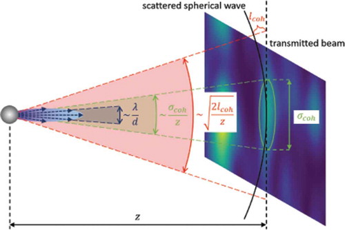
The staggered interference between the main beam and the randomly-phased plane waves with angular distribution $\tilde{S}$ generates the stochastic intensity distribution of heterodyne speckles. The characteristic length scale of such intensity fluctuations (the speckle size) is therefore given by:

(21) $d_{sp}(z)=\frac{2\pi }{q_{\mathrm{m}\mathrm{a}\mathrm{x}}(z)}=\frac{\lambda }{{\theta }_{\mathrm{m}\mathrm{a}\mathrm{x}}(z)}{\theta }_{\mathrm{m}\mathrm{a}\mathrm{x}}(z)=min\left\{\frac{\lambda }{d},\frac{{\sigma }_{\mathrm{c}\mathrm{o}\mathrm{h}}}{z},\sqrt{\frac{2l_{\mathrm{c}\mathrm{o}\mathrm{h}}}{z}}\right\}.$(21)

A summary is reported in Table 1, and effects on power spectra from the published literature are evidenced.

Table 1. Summary of the size of Heterodyne Near Field Speckles under different illumination conditions. The corresponding effects on power spectra are evidenced, as well as relevant examples from the published literature

	${\theta }_{\mathrm{m}\mathrm{a}\mathrm{x}}=\lambda /d$	${\theta }_{\mathrm{m}\mathrm{a}\mathrm{x}}={\sigma }_{\mathrm{c}\mathrm{o}\mathrm{h}}/z$	${\theta }_{\mathrm{m}\mathrm{a}\mathrm{x}}=(2l_{\mathrm{c}\mathrm{o}\mathrm{h}}/z{)}^{1/2}$
Speckle size	$d_{sp}=d$	$d_{sp}=\lambda z/{\sigma }_{\mathrm{c}\mathrm{o}\mathrm{h}}$	$d_{sp}=[{\lambda }^{2}z/(2l_{\mathrm{c}\mathrm{o}\mathrm{h}}){]}^{1/2}$
Scaling of power spectrum	None	$\mathrm{\Delta }\mathbf{x}=z\mathbf{q}/k$	$\mathrm{\Delta }t=z{q}^2/(2k^{2}c)$
Applications^a	Particle sizing	Spatial coherence	Temporal coherence
References	[14–24,30,31]	[28,29,32–36,39,40]	[28,29,36–38]

^aIn [25–27] (velocimetry), the speckle size is actually limited by the numerical aperture $NA$ of the collection optics. Thus, subjective speckles arise and ${\theta }_{\mathrm{m}\mathrm{a}\mathrm{x}}\sim NA$ in Equation 21(21) $d_{sp}(z)=\frac{2\pi }{q_{\mathrm{m}\mathrm{a}\mathrm{x}}(z)}=\frac{\lambda }{{\theta }_{\mathrm{m}\mathrm{a}\mathrm{x}}(z)}{\theta }_{\mathrm{m}\mathrm{a}\mathrm{x}}(z)=min\left\{\frac{\lambda }{d},\frac{{\sigma }_{\mathrm{c}\mathrm{o}\mathrm{h}}}{z},\sqrt{\frac{2l_{\mathrm{c}\mathrm{o}\mathrm{h}}}{z}}\right\}.$(21) . In [41–83] (X-ray wavefront sensing and X-ray phase-contrast imaging), both the size of the scatterers and the finite extent of the coherence areas might simultaneously play a role.

6. Conclusions

Heterodyne Near Field Speckles arise from the peculiar self-referencing interference between the faint, randomly-phased spherical waves scattered by a disordered sample and the intense trans-illuminating beam. With coherent light, the self-referencing layout allows to preserve phase information, thus paving the way to direct assessment of the scattered field. With partially coherent light, it proves of utmost importance to probe the coherence properties of the incoming wavefront.

Originally introduced in the optical domain, the fundamentals of the technique are largely wavelength independent, thus making the method appealing for large-scale facilities such as synchrotrons and FELs.

Starting from a basic description for the case of coherent laser light, we have developed a formalism based on Fourier Optics to quantitatively describe the power spectrum and the autocorrelation function of Heterodyne Near Field Speckles. Extension to the case of partially coherent radiation has been discussed, and emphasis has been given to the speckle size under different illumination conditions.

We have reviewed earlier and state-of-the-art development of Heterodyne Near Field Speckles, such as low-angle static and dynamic scattering measurements either in the visible range or at X-ray wavelengths. In the optical domain, the method can be applied to velocimetry measurements as well. At X-ray wavelengths, the same principles are exploited for X-ray wavefront sensing and X-ray phase contrast imaging. Applications to both transverse and longitudinal coherence characterization of synchrotron radiation beams have also been discussed. Thus, an important resource of Heterodyne Near Field Speckles is the wealth of information available to investigate a variety of physical and chemical systems, as well as to perform wavefront diagnostics of synchrotron and FEL beams.

In spite of the wide range of applications and wavelength domains, we have evidenced the equivalence between the coherent case and the partially coherent case in terms of illumination conditions. More in general, we have provided a unified and simple description of Heterodyne Near Field Speckles based on Fourier Optics.

Finally, it is important to emphasize how Heterodyne Near Field Speckles share many common aspects with different research areas, such as astronomical observations, holography and TEM imaging, thus proving the encompassing nature of the underlying physical principles.

Acknowledgments

The authors gratefully acknowledge the anonymous referee for the interest shown towards this work, for the enormous investment of time in carefully reading the manuscript, and for the useful comments and suggestions provided. The authors also acknowledge support from the University of Milan through the APC initiative.

Disclosure statement

No potential conflict of interest was reported by the authors.

References

- Dainty JC. Laser speckle and related phenomena. New York: Springer-Verlag Berlin Heidelberg; 1975.
- Goodman JW. Speckle Phenomena in Optics. Englewood: Ben Roberts & Company; 2007.
- Newton I. Optiks. New York: reprinted by Dover Press; 1952.
- Exner K, Sitzungsber. Kaiserl. Akad. Wiss. 1877;76:522.
- Exner K, Wiedemanns. Ann. Physik. 1880;9:239.
- Von Laue M, Sitzungsber. Akad. Wiss. 44 (1914), p. 1144.
- See, for example, La Mort de Casagemas by Picasso, Pablo (oil on wood, 1901, Musée Picasso, Paris), Il Sole by Pellizza da Volpedo, Giuseppe (oil on canvas, 1904, Galleria Nazionale d’Arte Moderna, Rome), Sole Nascente sul Fiume by Olivero, Matteo (oil on canvas, 1907-1910), Lampada ad Arco by Balla, Giacomo (oil on canvas, 1909-1911, Museum of Modern Art, New York).
- Interestingly, the eye of the observer itself provides the random medium in these cases. To support this statement, one can perform some convincing experiments. By looking at sunlight through a dense foliage, elongated white light speckles can be observed. Taking pictures of such speckles with a reflex camera is likely to fail, unless e.g. moisture is breathed on the front lens to make its surface irregular.
- Born M, Wolf E. Priciples of Optics. Oxford: Pergamon Press; 1970.
- Mandel L, Wolf E. Optical coherence and quantum optics. Cambridge: Cambridge University Press; 1995.
- Goodman JW. Statistical Optics. New York: John Wiley & Sons, Inc; 2000.
- De Haas WJ, Koninklighe. Acad. van Wetenschager. 1918;20:1278.
- Parry G, Some effects of surface roughness on the appearance of speckle in polychromatic light. Opt. Commun. 1974;12:75–46.
- Brogioli D, Vailati A, Giglio M. Heterodyne near-field scattering. Appl. Phys. Lett. 2002;81:4109–4111.
- Giglio M, Brogioli D, Potenza MAC, et al. Near field scattering. Phys Chem Chem Phys. 2004;6:1547–1550.
- Ferri F, Magatti D, Pescini D, et al., Heterodyne near-field scattering: A technique for complex fluids. Phys. Rev. E. 2004;70:041404.
- Brogioli D, Vailati A, Giglio M. A schlieren method for ultra-low–angle light scattering measurements. Europhys. Lett. 2003;63:220–225.
- Potenza MAC, Magatti D, Pescini D, et al., Proc. of SPIE Bellingham, WA.2004;5249: 461–470.
- Potenza MAC, Pescini D, Magatti D, et al. A new particle sizing technique based on near field scattering. Nuclear Physics B (Proc. Suppl.). 2006;150: 334–338.
- Magatti D, Alaimo MD, Potenza MAC, et al. Dynamic heterodyne near field scattering. Appl Phys Lett. 2008;92:241101.
- Mazzoni S, Potenza MAC, Alaimo MD, et al. SODI-COLLOID: a combination of static and dynamic light scattering on board the International Space Station. Rev Sci Instrum. 2013;84:043704.
- Potenza MAC, Manca A, Veen SJ, et al., EPL. 2014;106:68005.
- Escobedo-Sanchez MA, Rojas-Ochoa LF, Laurati M, et al. Investigation of moderately turbid suspensions by heterodyne near field scattering. Soft Matter. 2017;13:5961–5969.
- Cremonesi L, Siano M, Paroli B, et al. Near field scattering for samples under forced flow. Rev Sci Instrum. 2020;91:075108.
- Alaimo MD, Magatti D, Ferri F, et al. Heterodyne speckle velocimetry. Appl Phys Lett. 2006;88:191101.
- Potenza MAC, Alaimo MD, Pescini D, et al. A new technique for fluid velocimetry based on near field scattering. Opt. Laser Eng. 2006;44:722–731.
- Alaimo MD, Potenza MAC, Magatti D, et al. Heterodyne speckle velocimetry of Poiseuille flow. J Appl Phys. 2007;102:073113.
- Siano M, Paroli B, Chiadroni E, et al. Measurement of power spectral density of broad-spectrum visible light with heterodyne near field scattering and its scalability to betatron radiation. Opt Express. 2015;23:32888–32896.
- Siano M, Paroli B, Chiadroni E, et al., Note: Nanosecond LED-based source for optical modeling of scintillators illuminated by partially coherent X-ray radiation. Rev. Sci. Instrum. 87 (2016), p.126104.
- Cerbino R, Peverini L, Potenza MAC, et al. X-ray-scattering information obtained from near-field speckle. Nat. Phys. 2008;4:238–243.
- Lu X, Mochrie SGJ, Narayanan S, et al. X-ray near-field speckle: implementation and critical analysis. J. Synchrotron Rad. 2011;18:823–834.
- Alaimo MD, Potenza MAC, Manfredda M, et al. Probing the transverse coherence of an undulator X-ray beam using brownian particles. Phys Rev Lett. 2009;103:194805.
- Alaimo MD, Anania MP, Artioli M, et al. Mapping the transverse coherence of the self amplified spontaneous emission of a free-electron laser with the heterodyne speckle method. Opt Express. 2014;22:30013–30023.
- Manfredda M, Alaimo MD, Giglio M, et al. Probing transverse coherence with the heterodyne speckle approach: overview and perspectives. Phys Procedia. 2015;62:59–64.
- Kashyap Y, Wang H, Sawhney K, Phys. Rev. A. 2015;92:033842.
- Siano M, Paroli B, Manfredda M, et al., Proc. of SPIE. Prague, Czech Republic, 2015.
- Siano M, Paroli B, Potenza MAC, et al., Proc. of IBIC. IBIC, Barcelona, Spain, 2016.
- Siano M, Paroli B, Potenza MAC, et al. Characterizing temporal coherence of visible synchrotron radiation with heterodyne near field speckles. Phys. Rev. Accel. Beams. 2017;20: 110702.
- Mazzoni S, Roncarolo F, Trad G, et al., Proc. of IBIC. Shanghai, China, 2018.
- Siano M, Paroli B, Potenza MAC, et al., Proc. of IBIC. Malmo, Sweden, 2019.
- Berujon S, Ziegler E, Cerbino R, et al. Two-dimensional X-ray beam phase sensing. Phys Rev Lett. 2012;108:158102.
- Berujon S, Ziegler E, Cloetens P. X-ray pulse wavefront metrology using speckle tracking. J. Synchrotron Rad. 2015;22:886–894.
- Wang H, Kashyap Y, Sawhney K. Speckle based X-ray wavefront sensing with nanoradian angular sensitivity. Opt Express. 2015;23:23310–23317.
- Seaberg M, Cojocaru R, Berujon S, et al. Wavefront sensing at X-ray free-electron lasers. J. Synchrotron Rad. 2019;26:1115–1126.
- Sawhney K, Alcock S, Sutter J, et al. Characterisation of a novel super-polished bimorph mirror. J. Phys. Conf. Ser. 2013;425:052026.
- Berujon S, Wang H, Sawhney KJS. At-wavelength metrology using the X-ray speckle tracking technique: case study of a X-ray compound refractive lens. J. Phys. Conf. Ser. 2013;425:052020.
- Berujon S, Wang H, Alcock S, et al. At-wavelength metrology of hard X-ray mirror using near field speckle. Opt Express. 2014;22:6438–6446.
- Wang H, Kashyap Y, Laundy D, et al. J. Synchrotron Rad. 2015;22:925–929.
- Wang H, Sutter J, Sawhney K. Advanced in situ metrology for x-ray beam shaping with super precision. Opt Express. 2015;23:1605–1614.
- Kashyap Y, Wang H, Sawhney K. J. Synchrotron Rad. 2016;23:1131–1136.
- Kashyap Y, Wang H, Sawhney K. Speckle-based at-wavelength metrology of X-ray mirrors with super accuracy. Rev. Sci. Instrum. 2016;87:052001.
- Wang H, Zhou T, Kashyap Y, et al., Speckle-based at-wavelength metrology of X-ray optics at Diamond Light Source. Proc. of SPIE. 2017;10388:103880I.
- Zdora M-C, Zanette I, Zhou T, et al. At-wavelength optics characterisation via X-ray speckle- and grating-based unified modulated pattern analysis. Opt Express. 2018;26:4989–5004.
- Berujon S, Cojocaru R, Piault P, et al. X-ray optics and beam characterization using random modulation: theory. J. Synchrotron Rad. 2020;27:284–292.
- Berujon S, Cojocaru R, Piault P, et al. X-ray optics and beam characterization using random modulation: experiments. J. Synchrotron Rad. 2020;27:293–304.
- Morgan KS, Paganin DM, Siu KKW. X-ray phase imaging with a paper analyzer. Appl Phys Lett. 2012;100:124102.
- Berujon S, Wang H, Sawhney K, Phys. Rev. A. 2012;86:063813.
- Berujon S, Wang H, Pape I, et al. X-ray phase microscopy using the speckle tracking technique. Appl Phys Lett. 2013;102:154105.
- Wang H, Berujon S, Pape I, et al. X-ray microscopy using two phase contrast imaging techniques: two dimensional grating interferometry and speckle tracking. J Phys Conf Ser. 2013;463:012042.
- Zanette I, Zhou T, Burvall A, et al. Speckle-Based X-ray phase-contrast and dark-field imaging with a laboratory source. Phys Rev Lett. 2014;112:253903.
- Aloision IA, Paganin DM, Wright CA, et al. Exploring experimental parameter choice for rapid speckle-tracking phase-contrast X-ray imaging with a paper analyzer. J. Synchrotron Rad. 2015;22:1279–1288.
- Zhou T, Zanette I, Zdora M-C, et al. Speckle-based x-ray phase-contrast imaging with a laboratory source and the scanning technique. Opt. Lett. 2015;40:2822–2825.
- Berujon S, Ziegler E, Phys. Rev A. 2015;92:013837.
- Wang H, Kashyap Y, Sawhney K. Hard-X-ray directional dark-field imaging using the speckle scanning technique. Phys Rev Lett. 2015;114:103901.
- Wang H, Berujon S, Herzen J, et al. X-ray phase contrast tomography by tracking near field speckle. Sci Rep. 2015;5:8762.
- Zanette I, Zdora M-C, Zhou T, et al., PNAS 2015;112:12569–12573.
- Zdora M-C, Thibault P, Pfeiffer F, et al. Simulations of x-ray speckle-based dark-field and phase-contrast imaging with a polychromatic beam. J Appl Phys. 2015;118:113105.
- Kashyap Y, Wang H, Sawhney K. Experimental comparison between speckle and grating-based imaging technique using synchrotron radiation X-rays. Opt Express. 2016;24:18664–18673.
- Zdora M-C, Thibault P, Herzen J, et al., AIP Conf. Proc. 2016;1696:020016.
- Wang H, Kashyap Y, Sawhney K. Quantitative X-ray dark-field and phase tomography using single directional speckle scanning technique. Appl Phys Lett. 2016;108:124102.
- Berujon S, Ziegler E. X-ray multimodal tomography using speckle-vector tracking. Phys. Rev. Appl. 2016;5: 044014.
- Wang H, Kashyap Y, Sawhney K. From synchrotron radiation to lab source: advanced speckle-based X-ray imaging using abrasive paper. Sci Rep. 2016;6:20476.
- Wang F, Wang Y, Wei G, et al. Speckle-tracking X-ray phase-contrast imaging for samples with obvious edge-enhancement effect. Appl Phys Lett. 2017;111:174101.
- Zdora M, Thibault P, Rau C, et al. Characterisation of speckle-based X-ray phase-contrast imaging. J. Phys. Conf. Ser. 2017;849:012024.
- Romell J, Zhou T, Zdora M, et al. Comparison of laboratory grating-based and speckle-tracking x-ray phase-contrast imaging. J Phys Conf Ser. 2017;849:012035.
- Berujon S, Ziegler E, Phys. Rev. A. 2017;95:063822.
- Vittoria FA, Endrizzi M, Olivo A. Retrieving the ultrasmall-angle X-ray scattering signal with polychromatic radiation in speckle-tracking and beam-tracking phase-contrast Imaging. Phys. Rev. Appl. 2017;7: 034024.
- Zdora M-C, Thibault P, Zhou T, et al., Phys. Rev. Lett. 2017;118:203903.
- Zdora M-C. State of the Art of X-ray speckle-based phase-contrast and dark-field imaging. J Imaging. 2018;4:60.
- Paganin DM, Labriet H, Brun E, et al., Phys. Rev. A. 2018;98:053813.
- Zdora M-C, Zanette I, Walker T, et al. X-ray phase imaging with the unified modulated pattern analysis of near-field speckles at a laboratory source. Appl. Opt. 2020;59:2270–2275.
- Pavlov KM, Paganin DM, Rouge-Labriet H, et al.. Single-shot X-Ray speckle-based imaging of a single-material object. Phys. Rev. Appl. 13:2020; 054023.
- Tian N, Jiang H, Li A, et al. Influence of diffuser grain size on the speckle tracking technique. J. Synchrotron Rad. 2020;27:146–157.
- Goodman JW. Introduction to Fourier Optics. Englewood: Ben Roberts & Company; 2007.
- Paganin DM. Coherent X-ray Optics. Oxford: Oxford University Press; 2006.
- By virtue of the Huygens-Fresnel principle, et(x, z)= ∫e0(x’) h(x – x’, z) dx’, where h(x,z) = exp(ikz) exp[ik|x|2/(2z)] in paraxial conditions. The convolution kernel h becomes highly oscillatory for |x|>(λz)1/2, thus making the convolution integral vanish. If D≫(λz)1/2, h acts as a Dirac δ-distribution and et(x, z) = e0(x)exp(ikz).
- Saleh BEA, Teich MC. Fundamentals of Photonics. New York: John Wiley & Sons, Inc; 1991.
- At variance, the superposition of two laterally-displaced spherical waves as in the Young double-pinhole experiment generates parallel fringes with a fixed spacing. It is equivalent to the interference between two tilted plane waves.
- Gabor D. A new microscopic principle. Nature. 1948;161:777.
- Gabor D, Proc. Roy. Soc. London. 1949;197:454.
- Gabor D, Microscopy by Reconstructed Wave Fronts: II. Proc. Phys. Soc. 1951;64:449.
- Williams DB, Carter CB. Transmission electron microscopy. New York: Plenum Press; 1996.
- Kim MK. Principles and techniques of digital holographic microscopy. SPIE Review. 2010;1:018005.
- Vu X, Hong J, Liu C, et al. Review of digital holographic microscopy for three-dimensional profiling and tracking. Opt Eng. 2014;53:112306.
- Tahara T, Quan X, Otami R, et al. Digital holography and its multidimensional imaging applications: a review. Microscopy. 2018;67:55–67.
- Shao Y, Lu X, Konijnenberg S, et al. Spatial coherence measurement and partially coherent diffractive imaging using self-referencing holography. Opt Express. 2018;26:4479–4490.
- McNulty I, Nucl. Instrum. Methods. Phys. Res. A. 347 (1994), p.170.
- Eisebitt S, Luning J, Schlotter WF, et al. Lensless imaging of magnetic nanostructures by X-ray spectro-holography. Nature. 2004;432:885–888.
- Momose A. Recent Advances in X-ray Phase Imaging. Jpn. J. Appl. Phys. 2005;44:6355–6367.
- Marchesini S, Boutet S, Sakdinawat AE, et al. Massively parallel X-ray holography. Nat Photonics. 2008;2:560–563.
- Chapman HN, Nugent KA. Coherent lensless X-ray imaging. Nat Photonics. 2010;4:833–839.
- Gorniak T, Heine R, Mancuso AP, et al. X-ray holographic microscopy with zone plates applied to biological samples in the water window using 3rd harmonic radiation from the free-electron laser FLASH. Opt Express. 2011;19:11059–11070.
- Martin AV, D’Alfonso AJ, Wang F, et al. X-ray holography with a customizable reference. Nat Commun. 2014;5:4661.
- Gorkhover T, Ulmer A, Ferguson K, et al. Femtosecond X-ray Fourier holography imaging of free-flying nanoparticles. Nat Photonics. 2018;12:150–153.
- Medecki H, Tejnil E, Goldberg KA, et al. Phase-shifting point diffraction interferometer. Opt. Lett. 1996;21:1526–1528.
- Momose A. Phase-sensitive imaging and phase tomography using X-ray interferometers. Opt Express. 2003;11:2303–2314.
- Leitenberger W, Wendrock H, Bischoff L, et al. Pinhole interferometry with coherent hard X-rays. J. Synchrotron Rad. 2004;11:190–197.
- Homer P, Rus B, Polan J, Measurements of x-ray laser wavefront profile using PDI technique. Proc. of SPIE. 2007;6702:670211.
- Malyshev IV, Chkhalo NI, Akhsahalian AD, et al. Surface shape measurement of mirrors in the form of rotation figures by using point diffraction interferometer. J. Mod. Opt. 2017;64:413–421.
- Takeuchi S, Kakuchi O, Yamazoe K, et al., Visible light point-diffraction interferometer for testing of EUVL optics. Proc. of SPIE 2006;6151:61510E.
- Wang D, Wang F, Zou H, et al. Analysis of diffraction wavefront in visible-light point-diffraction interferometer. Appl. Opt. 2013;52:7602–7608.
- Gao F, O’Donoghue T, Wang W. Full-field analysis of wavefront errors in point diffraction interferometer with misaligned Gaussian incidence. Appl. Opt. 2020;59:210–216.
- Giglio M, Carpineti M, Vailati A. pace Intensity Correlations in the Near Field of the Scattered Light: A Direct Measurement of the Density Correlation Function g(r). Phys Rev Lett. 2000;85:1416–1419.
- Giglio M, Carpineti M, Vailati A, et al. Near-field intensity correlations of scattered light. Appl. Opt. 2001;40:4036–4040.
- Trainoff SP, Cannell DS. Physical optics treatment of the shadowgraph. Phys. Fluids. 2002;14: 1340–1363.
- Cloetens P, Ludwig W, Baruchel J, et al. Holotomography: quantitative phase tomography with micrometer resolution using hard synchrotron radiation x rays. Appl. Phys. Lett. 1999;75:2912–2914.
- Zabler S, Cloetens P, Guigay J-P, et al. Optimization of phase contrast imaging using hard x rays. Rev Sci Instrum. 2005;76:073705.
- Salditt T, Giewekemeyer K, Fuhse C, et al. Projection phase contrast microscopy with a hard x-ray nanofocused beam: defocus and contrast transfer. Phys Rev B. 2009;79:184112.
- Van De Hulst HC. Light scattering by small particles. New York: Dover Publications, Inc; 1981.
- Potenza MAC, Sabareesh KPV, Carpineti M, et al. How to measure the optical thickness of scattering particles from the phase delay of scattered waves: application to turbid samples. Phys Rev Lett. 2010;105:193901.
- Li WB, Segrè PN, Gammon RW, et al., Physica A 204 (1994), p.399.
- Berne BJ, Pecora R. Dynamic light scattering. New York: Dover Publications, Inc; 2000.
- Guo H, Narayanan T, Sztuchi M, et al. Reversible phase transition of colloids in a binary liquid solvent. Phys Rev Lett. 2008;100:188303.
- Bonn D, Otwinowski J, Sacanna S, et al., Direct Observation of Colloidal Aggregation by Critical Casimir Forces. Phys. Rev. Lett. 2009;103:156101.
- Veen SJ, Antoniuk O, Weber B, et al. Colloidal aggregation in microgravity by critical casimir forces. Phys. Rev. Lett. 2012;109:248302.
- Cerbino R, Vailati A. Near-field scattering techniques: novel instrumentation and results from time and spatially resolved investigations of soft matter systems. Curr. Opin. Colloid Interface Sci. 2009;14:416–425.
- In the far zone, the speckles do not move upon particle motions, but simply fluctuate stochastically in time. This is due to the fact that each speckle in the far field is the result of contributions from the entire illuminated sample, and therefore no correspondence between speckles and particles is possible.
- Buzzaccaro S, Secchi E, Piazza R. Ghost particle velocimetry: accurate 3D flow visualization using standard lab equipment. Phys Rev Lett. 2013;111:048101.
- Secchi E, Rusconi R, Buzzaccaro S, et al., Intermittent turbulence in flowing bacterial suspensions. J. R. Soc. Interface. 2016;13:20160175.
- Eberhard U, Seybold HJ, Secchi E, et al. Mapping the local viscosity of non-Newtonian fluids flowing through disordered porous structures. Sci. Rep. 2020;10:11733.
- Kuiper GP, Middlehurst BM. Telescopes. Chicago: The University of Chicago Press; 1960.
- Keller G, Protheroe WM, Barnhart PE, et al., Reprint No. 39. Perkins Observatory, Delaware, 1956.
- Mikesell AH, Hoag AA, Hall JS. The scintillation of starlight*. J. Opt. Soc. America. 1951;41: 689.
- Protheroe WM, Contr. Perkins Obs. No. II-4, Delaware, 1955.
- Gifford F, Mikesell AH, Weather. 19538:195.
- Mikesell AH, Pub. U. S. Naval Obs. 195517:139.
- Barnhart PE, Keller G, Mitchell WE, Report TR59-291, Air Force Cambridge Research Center: Bedford, Mass, 1959.
- Spence JCH. Experimental high-resolution electron microscopy. Oxford: Oxford University Press; 1988.
- Scherzer O. The theoretical resolution limit of the electron microscope. J. Appl. Phys. 1949;20:20–29.
- Hashimoto H, Endoh H. Electron Diffraction 1927-1977. Bristol and London: The Institute of Physics; 1978.
- Krivanek OL. A method for determining the coefficient of spherical aberration from a single electron micrograph. Optik. 1976;45:97.
- Cerbino R, Peverini L, Potenza MAC, et al. X-ray-scattering information obtained from near-field speckle. Nat. Phys. 2008;4:238–243. [Suppl. Mat].
- Dubois F, Joannes L, Legros J-C. Improved three-dimensional imaging with a digital holography microscope with a source of partial spatial coherence. Appl. Opt. 1999;38:7085–7094.
- Dubois F, Minetti C, Monnom O, et al. Pattern recognition with a digital holographic microscope working in partially coherent illumination. Appl. Opt. 2002;41:4108–4119.
- Dubois F, Novella Requena M-L, Minetti C, et al. Partial spatial coherence effects in digital holographic microscopy with a laser source. Appl. Opt. 2004;43:1131–1139.
- Dubois F, Callens N, Yourassowsky C, et al. Digital holographic microscopy with reduced spatial coherence for three-dimensional particle flow analysis. Appl. Opt. 2006;45:864–871.
- Minetti C, Callens N, Coupier G, et al. Fast measurements of concentration profiles inside deformable objects in microflows with reduced spatial coherence digital holography. Appl. Opt. 2008;47:5305–5314.
- Dubois F, Yourassowsky C, Callens N, et al. Applications of digital holographic microscopes with partially spatial coherence sources. J. Phys. Conf. Ser. 2008;139:012027.
- Dubois F, Yourassowsky C, Off-axis multispectral digital holographic microscope with partially coherent illumination. Proc. of SPIE. 20128429:84291E.
- Minetti C, Podgorski T, Coupuier G, et al., Dynamics of vesicle suspension in shear flow between walls by digital holographic microscopy with a spatially reduced coherent source. Proc. of SPIE. 20128429 :84291I.
- Dohet-Eraly J, Yourassowsky C, El Mallahi A, et al. Quantitative assessment of noise reduction with partial spatial coherence illumination in digital holographic microscopy. Opt. Lett. 2016;41:111–114.
- Dohet-Eraly J, Yourassowsky C, El Mallahi A, et al., Partial spatial coherence illumination in digital holographic microscopy: quantitative analysis of the resulting noise reduction. Proc. of SPIE. 2016;9890:989004.
- Manfredda M, Siano M, Paroli B, et al., in preparation.
- Pfeiffer F, Bunk O, Schulze-Briese C, et al. Shearing interferometer for quantifying the coherence of hard X-ray beams. Phys Rev Lett. 2005;94:164801.
- Weitkamp T, Diaz A, David C, et al. X-ray phase imaging with a grating interferometer. Opt Express. 2005;12:6296–6304.
- Pfeiffer F, Bech M, Bunk O, et al. Hard-X-ray dark-field imaging using a grating interferometer. Nat Mater. 2008;7:134–137.
- Cloetens P, Guigay JP, De Martino C, et al. Fractional Talbot imaging of phase gratings with hard x rays. Opt. Lett. 1997;22:1059–1061.
- Momose A, Kawamoto S, Koyama I, et al. Demonstration of X-Ray Talbot Interferometry. Jpn. J. Appl. Phys. 2003;42:L866–L868.
- Guigay J-P, Zabler S, Cloetens P, et al. The partial Talbot effect and its use in measuring the coherence of synchrotron X-rays. J. Synchrotron Rad. 2004;11:476–482.
- Engelhardt M, Kottler C, Bunk O, et al. The fractional Talbot effect in differential x-ray phase-contrast imaging for extended and polychromatic x-ray sources. J. Microsc. 2008;232:145–157.
- Momose A, Yashiro W, Maikusa H, et al. High-speed X-ray phase imaging and X-ray phase tomography with Talbot interferometer and white synchrotron radiation. Opt Express. 2009;17:12540–12545.
- Yashiro W, Terui Y, Kawabata K, et al. On the origin of visibility contrast in x-ray Talbot interferometry. Opt Express. 2010;18:16890–16901.
- Salditt T, Kalbfleisch S, Osterhoff M, et al. Partially coherent nano-focused x-ray radiation characterized by Talbot interferometry. Opt Express. 2011;19:9656–9675.
- Nugent KA. Coherent methods in the X-ray sciences. Adv Phys. 2010;59:1–99.
- Cipelletti L, Carpineti M, Giglio M. Fractal morphology, spatial order, and pore structure in microporous membrane filters. Langmuir. 1996;12:6446–6451.
- Manfredda M, Probing synchrotron radiation coherence: the heterodyne speckle approach, Ph.D. thesis, Milan, 2012, https://air.unimi.it/handle/2434/172631
- Gutt C, Wochner P, Fisher B, et al. Single shot spatial and temporal coherence properties of the SLAC linac coherent light source in the hard X-ray regime. Phys Rev Lett. 2012;108:024801.
- Lee S, Roseker W, Gutt C, et al. Single shot speckle and coherence analysis of the hard X-ray free electron laser LCLS. Opt Express. 2013;21:24647–24664.
- Lehmkuhler F, Gutt C, Fischer B, et al. Single shot coherence properties of the free-electron laser SACLA in the hard X-ray Regime. Sci Rep. 2014;4:5234.
- Geloni G, Saldin E, Schneidmiller E, et al. Transverse coherence properties of X-ray beams in third-generation synchrotron radiation sources. Nucl Instrum Methods Phys Res A. 2008;588:463–493.
- Paroli B, Potenza MAC, Advances in Physics. X 2(2017), p.978–1004.
- Geloni G, Serkez S, Khubbutdinov R, et al. Effects of energy spread on brightness and coherence of undulator sources. J. Synchrotron Rad. 2018;25:1335–1345.
- Thomas C, Dudin P, Hoesch M. Coherence of a near diffraction limited undulator synchrotron radiation source. Opt. Commun. 2016;359:171–176.
- Paroli B, Chiadroni E, Ferrario M, et al., Asymmetric lateral coherence of betatron radiation emitted in laser-driven light sources. EPL 2015;111::44003.
- Paroli B, Chiadroni E, Ferrario M, et al. A systematic study of the asymmetric lateral coherence of radiation emitted by ultra-relativistic particles in laser-driven accelerators. Nucl Instrum Methods Phys Res A. 2016;839:1–5.
- Paroli B, Bravin E, Mazzoni S, et al., A modified two-slit interferometer for characterizing the asymmetric lateral coherence of undulator radiation. EPL 2016;115:14004.
- Paroli B, Siano M, Potenza MAC. A symmetric lateral coherence allows precise wavefront characterization. EPL. 2018;122:44001.
- Paroli B, Cirella A, Debrot I, et al. Asymmetric lateral coherence of OAM radiation reveals topological charge and local curvature. J Opt. 2018;20:075605.
- Paroli B, Siano M, Potenza MAC. The local intrinsic curvature of wavefronts allows to detect optical vortices. Opt Express. 2019;27:17550–17560.
- Paroli B, Siano M, Teruzzi L, et al. Single-shot measurement of phase and topological properties of orbital angular momentum radiation through asymmetric lateral coherence. Phys. Rev. Accel. Beams. 2019;22: 032901.
- Paroli B, Siano M, Potenza M. Measuring the topological charge of orbital angular momentum radiation in single-shot by means of the wavefront intrinsic curvature. Appl. Opt. 2020;59:5258–5264.
- Paroli B, Siano M, Potenza MAC. A composite beam of radiation with orbital angular momentum allows effective local, single-shot measurement of topological charge. Opt Commun. 2020;459:125049.
- Berto P, Rigneault H, Guillon M. Wavefront sensing with a thin diffuser. Opt. Lett. 2017;42:5117–5120.
- Gatti A, Magatti D, Ferri F .Three-dimensional coherence of light speckles: theory. Phys Rev. 2008;78:063806. doi:https://doi.org/10.1103/PhysRevA.78.063806.
- Magatti D, Gatti A, Ferri F .Three-dimensional coherence of light speckles: experiment. Phys Rev.2009;79:053831. doi:https://doi.org/10.1103/PhysRevA.79.053831.