Combining recorded failures and expert opinion in the development of ANN pipe failure prediction models

ABSTRACT

Buried pipes comprise a significant portion of assets of a water utility. With time, these pipes inevitably fail. Failure prediction enables infrastructure managers to estimate long-term failure trends for budgetary planning purposes and identify critical pipes for preventive intervention planning. For short-term prioritization, machine learning based algorithms appear to have superior predictive performance compared to traditional survival analysis based models. These models are typically stratified by material resulting in the exclusion of newer pipe materials such as polyethylene and corrosion-protected ductile iron, despite their prevalence in modern networks. In this paper, an application of an existing methodology is presented to estimate time to next failure using artificial neural networks (ANNs). The novelties of the approach are 1) including material as an input parameter instead of training several material-specialized models and, 2) addressing right-censored data by combining soft and hard deterioration data. The model is intended for use in short-term prioritization.

KEYWORDS:

• Artificial neural networks
• failure prediction
• water distribution networks

1. Introduction

Water distribution networks are underground networks of pipes that transport drinking quality water at sufficient pressure and quantity at all times to the public. These pipes inevitably fail for a number of reasons, such as frost heave, corrosion, and poor installation. The exact mechanisms are not fully understood, and thus failures are very difficult to predict (Balvant Rajani & Kleiner, 2001).

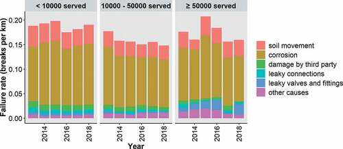
Researchers have identified numerous contributing factors to pipe deterioration. These can be conveniently divided into physical factors, operational factors, and environmental factors (Al-Barqawi & Zayed, 2006; Infraguide, 2002). Physical factors are related to the pipe itself (e.g., age, material, diameter, etc.). Operational factors describe the operational characteristics of the pipe in the distribution network (internal pressure, pressure fluctuations, water characteristics, etc.) and environmental factors relate to the pipe’s environment (e.g., soil type, groundwater levels, etc.). As noted by Folkman (2018), water main failure rates are the most important indicator of pipe structural condition. His survey of North American water utilities found that the presence of corrosive soils was a major contributing factor to pipe failure. In addition, smaller utilities (less than 320 km of installed water mains) reported twice the failure rate of larger ones (more than 1600 km of installed water mains), which was attributed to differences in funding levels and resulting asset management practices. Figure 1 shows the overall pipe failure rate for water utilities in Switzerland by the size of the served population and reported cause excluding service lines (SVGW, 2014, 2015b, 2016, 2017, 2018, 2019). Corrosion and soil movement consistently account for the majority of pipe failures with relatively minor differences in failure rate for Swiss utilities of different sizes. A direct comparison with Folkman (2018) is not possible as Swiss utilities are smaller. The largest network contains 1265 km of water mains, and only eight utilities manage networks with more than 320 km of buried water mains (SVGW, 2015a, 2019). Overall, the failure rate has fluctuated between 0.15 and 0.20 breaks/km/year in recent years, which is considered moderate (DVGW, 2006; SVGW, 2012).

Figure 1. Failure rate by utility size and reported cause in Switzerland.

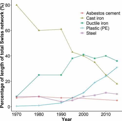
Beginning with Shamir and Howard (1979), a large number of pipe failure prediction models have been developed over the last 40 years, and several comprehensive reviews have been published summarizing the approaches (Kleiner & Rajani, 2001; Balvant Rajani & Kleiner, 2001; Scheidegger et al., 2015; Wilson et al., 2017; Yuan, 2016). These models have two primary objectives: estimating long-term failure rates associated with a given management strategy for budgetary planning purposes and identifying pipes that are likely to fail in the near future for prioritization (Lin & Yuan, 2019; Yuan, 2016). Recently, several independent research groups have observed that failure prediction models based on machine learning algorithms (MLAs) appear to perform better in identifying critical pipes in the short term and models based on survival analysis are better able to predict long-term failure trends (Caradot et al., 2018; Snider & McBean, 2019; Tscheikner-Gratl et al., 2019). Snider and McBean (2019) attributed this observation to the ability of survival analysis based models to correct for data that is left-truncated (i.e., failure data is only available from the point when recording began) or right-censored (i.e., future failures are unknown). Such models adjust the likelihood function used to calculate distribution parameters (Mailhot et al., 2000). Other approaches also exist such as simulating missing failure history data (Lin & Yuan, 2019), pooling data from multiple utilities to increase the data available for model calibration (Grigg, 2009; Renaud et al., 2009) and combining recorded failures with expert opinion using Bayesian inference (Scholten et al., 2013). MLA based models typically do not correct for left truncation and right censorship (Harvey et al., 2014; Sattar et al., 2019; Snider & McBean, 2019; Winkler et al., 2018). Snider and McBean (2019) investigated the effect of right censorship on model accuracy and found that its influence on results decreased as more pipes of a certain cohort failed. This indicates that right censorship is less of a concern for the failure prediction of older materials (e.g., cast iron) than new materials (e.g., polyethylene (PE)). This fact and the lack of recorded failure data often leads researchers to exclude newer pipe materials from deterioration modeling. This is problematic as these newer materials now account for a significant portion of water distribution networks. Figure 2 shows the material composition of Swiss water distribution networks over the last 50 years.

Figure 2. Pipe materials used in Swiss water distribution networks (SVGW, 2016).

In this study, the term newer materials refers to third-generation ductile iron (DI3) and PE. Ductile iron can be divided into two or three categories by level of corrosion protection. Based on the participating utility’s data, ductile iron is subdivided into three types: DI1 pipes, installed between 1955–1980, have no corrosion protection; DI2 pipes, installed between 1981–1993, have improved external corrosion protection; and DI3 (1985 – present) have extensive external and internal corrosion protection. PE can similarly be subdivided into different generations by creep rupture strength: PE50/PE63 were installed between 1957 and 1977; PE80 was installed between 1978 and 1990; and PE100/PE100 RC have been installed from 1991 to the present (Gressmann, 2020). Pipe manufacturers advertise an expected service life of 140 years for DI3 (vonRoll, 2020) and a minimum service life of 100 years for PE80/PE100/PE100 RC pipes based on material performance tests that investigated stress cracking and thermal aging (Gressmann, 2020; Hessel, 2007). A study commissioned by the German association of gas and water utilities (DVGW) in 2010 investigated the creep rupture curves and thermo-oxidative degradation of PE50/PE63 pipes after 30 years of operation and estimated a minimum remaining service life of 25 years (Wüst et al., 2010). Wallerath and Wehr (2014) estimated the technical service life to be 160 years for DI pipes (installed from 1980 onwards) and 154 years for PE pipes (installed from 1973 onwards) based on available water utility failure data from Germany. A two-parameter Weibull model was used in the analysis and the technical service life was defined as the time needed to reach a failure rate of 0.3 failures/km/year.

Although the failure rate of such materials is expected to remain low for decades, pipes made of newer materials are also prone to failure as conceptualized by the bathtub model (Kleiner & Rajani, 2001; Lin & Yuan, 2019; Rogers & Grigg, 2009; Scheidegger et al., 2015). This model expects an initial moderate failure rate for a pipe cohort due to failures caused by poor installation. Failure rate then decreases sharply and gradually rises with time due to deterioration. At the pipe level, once a pipe has failed, it is more likely to fail again, either due to the stress of the repair (Hu & Hubble, 2007; Scheidegger et al., 2015), the quality of the repair (i.e., repair work done in freezing weather will affect the quality of backfill and soil compaction (Hu & Hubble, 2007)) or continued deterioration. This is reflected in the literature, as failure prediction models have consistently found that failure history is the most important predictive attribute (Christodoulou et al., 2003; Harvey et al., 2014; Lin & Yuan, 2019; Sattar et al., 2019; Snider & McBean, 2019).

1.1. Artificial neural networks

Models based on artificial neural networks (ANNs) have been discussed in the scientific literature on failure prediction for over 20 years (see Table 1). Their use extends to a number of other Civil Engineering applications such as improving preliminary estimates of material quantities in construction projects (García de Soto et al., 2017) and predicting road accident frequency on a road network (García de Soto et al., 2018).

Table 1. Literature on the use of ANN for municipal pipe networks.

Reference	Inputs^1	Output	Models^2	ANN development	Performance comparison	Case study
Sacluti (1999)	11, 12	Area failure density	CI	MLP (1 hidden layer) with BEP. Coefficient of determination (R^2) used as performance criteria.	Number and data form of inputs varied.	22-yr dataset from Edmonton, CAN
Christodoulou et al. (2003); Christodoulou and Deligianni (2010)	1, 2, 4, 5, 33	Time to failure (days)	G	MLP (1 hidden layer). ANN integrated into a neuro-fuzzy decision framework.	1 vs. 2 hidden layers compared	10-yr dataset from New York City and Limassol, Cyprus
Ahn et al. (2005)	4, 11, 12, 13, 14	Network pipe failures	G	MLP (2 hidden layers) with BEP. Mean absolute error (MAE) used as performance criteria.	Not included	9-yr dataset from Seoul, South Korea
Najafi and Kulandaivel (2005)	1, 2, 4, 7, 15, 16, 17	Sewer pipe condition scale	G	MLP (1 hidden layer) with BEP. Root mean squared error (RMSE) used as performance criteria.	Number of nodes in hidden layer altered	Dataset from Atlanta, USA
Al-Barqawi and Zayed (2006)	1, 4, 6, 7, 15, 18, 19, 20,	Water pipe condition scale	G	MLP (1 hidden layer) with BEP. MAE, RMSE, average invalidity percent (AIP), and average validity percent (AVP) used as performance criteria	Not done	Dataset from three Canadian municipalities (Moncton, NB; Longueuil, QC; London, ON)
Achim et al. (2007)	1, 2, 3, 7, 21	Failure rate	G	MLP (2 hidden layers) with BEP. Coefficient of determination (R^2) used as performance criteria.	Inputs varied, number of hidden nodes varied	5-yr dataset from Victoria, Australia
Geem et al. (2007)	1, 4, 6, 7, 10, 15, 21, 22, 23, 30	Pipe condition index	G	MLP (1 hidden layer) with BEP. Coefficient of determination (R^2) used as performance criteria.	Not done	Data from water utility in South Korea
Tabesh et al. (2009)	1, 2, 7, 10, 15	Failure rate	G	MLP (1 and 2 hidden layers) with BEP. Index of agreement (IOA) and RMSE used as performance criteria.	Number of nodes in hidden layer	Data from city in Iran
Amaitik and Amaitik (2010)	7, 10, 15, 24, 25, 26, 27	Number of broken wires in PCCP	PCCP	MLP (2 hidden layers) with BEP. Coefficient of determination (R^2) used as performance criteria.	Not done	10-yr dataset of monitoring data from non-destructive techniques (NDT) of Libyan water network
Jafar, Shahrour, & Juran, (2007, 2010)	1, 2, 5, 6, 7, 8, 9, 31	Number of failures	P, AC, M, NoF, G	MLP (1 hidden layer). Coefficient of determination (R^2) and average squared error (ASE) used as performance criteria.	Not done	14-yr dataset of medium-sized city in Northern France.
Asnaashari et al. (2013)	1, 2, 4, 5, 6, 7, 29, 30	Failure rate	G	MLP (1 hidden layer). Coefficient of determination (R^2) and average squared error (ASE) used as performance criteria. 50:25:25 data split used.	Neurons in hidden layer. ANN compared to multiple linear regression (MLR)	20-yr dataset from Etobicoke, CAN.
Harvey et al. (2014)	1, 2, 3, 5, 6, 29, 30	Time to failure	AS, CI, DI	MLP (1 hidden layer). Correlation coefficient (R) and sum squared error (SSE) used as performance criteria. 70:15:15 data split used.	Initial weights and neurons in hidden layer	43-yr dataset from Scarborough, CAN.
Kutyłowska, (2015, 2017)	1, 2, 3, 4, 5, 17,32	Network failure rate per pipe type	DP, SL, G	Radial Basis Functions ANN (7-4-3) and MLP ANN (7–14-3) compared. 50:25:25 data split used in training phases. Absolute relative error and correlation coefficient used for performance.	Activation functions and ANN types	14 yr dataset from a city in Poland
Kerwin et al. (2018)	1, 3, 4, 5, 6, 10, 34	Time to failure	G, CI, DI	MLP (1 hidden layer) with BEP. 80:10:10 split	Material-specific compared to generalized model with MSE.	48-yr dataset from medium-sized utility (over 1000 km buried pipe)
Snider and McBean (2018)	1, 2, 3, 5, 6, 10, 28, 29, 34	Time to failure	DI	Developed in R using nnet package. 10-fold cross-validation repeated 3x.	Decision-tree based models (gradient boosting, random forest) compared to ANN	57-yr dataset from large North American utility
Sattar et al. (2019)	1, 2, 3, 5, 6, 28, 29	Failure rate	AC, CI, DI	MLP (one hidden layer) with extreme learning machine training algorithm instead of BEP	Four training algorithms compared	59-yr dataset from Scarborough, CAN

1. 1 – Diameter, 2 – Length, 3 – Construction year, 4 – Material, 5 – Number of previous failures, 6 – Soil type, 7 – Age at failure, 8 – Location underground, 9 – Pressure variation, 10 – Pressure head, 11 – Various air temperature measurements, 12 – Various water temperature measurements, 13 – Various soil temperature measurements, 14- Ratio of metered water, 15- Burial depth, 16 – Pipe slope (sewer), 17 – Pipe type, 18 – Road surface, 19 – Pipe failure rate, 20 – Hazen Williams coefficient, 21 – Geographical coordinates, 21 – Electric recharge, 22 – Bedding condition, 23 – Number of road lanes, 24 – Time between failures, 25 – Soil resistivity, 26 – Soil density, 27 – Wire characteristics, 28 – Cathodic protection, 29 – Cement mortar lining, 30 – Presence of pipe surface coating, 31 – Pipe thickness, 32 – Number of service lines, 33 – Various traffic parameters, 34 – Zoning

2. AC – Asbestos cement, CI – Cast iron, DI – Ductile iron, DP – Distribution pipes, G – Global/general, M – Metallic, NoF – Number of failures (high/low), P – plastic, PCCP – Pre-stressed concrete cylinder pipe (PCCP), SL – Service lines

ANNs are based on the structure of the human brain, where a dense network of neurons exchanges information via synapses. There are several types of ANNs, but the multi-layer perceptron (MLP) is the most common structure found in the literature on pipe failure prediction (see Table 1). An MLP is composed of an input layer, typically one hidden layer and an output layer. Each layer contains one or more perceptrons that process the weighted inputs and convert them to an output via an activation function. The ANN is taught through a process of supervised learning to perform a specific task. The algorithm used in this study is feed-forward backward error propagation (BEP), where the ANN is taught through an iterative process to predict the desired target value. The difference between the outputs and the target values is used to adjust the weights of the links between the layers. One complete instance of feed-forward backward error propagation is known as an epoch. The training process can take many epochs to complete, which happens when a tolerance value has been achieved, or a maximum number of epochs have been iterated. To avoid overtraining, the dataset is divided into a training set to train the ANN, a validation set to prevent overfitting, and a testing set to evaluate the ANN’s performance. For a more detailed explanation of ANNs, the reader is referred to Bishop (2007) or Mitchell (1997). Figure 3 illustrates the structure of an MLP and how a perceptron processes inputs.

Figure 3. (a) Schematic of a multi-layer perceptron (García de Soto et al., 2014); (b) Data conversion process in a perceptron (Adey et al., 2017).

When designing an ANN model, it is necessary to investigate the effects of model parameters on model performance. Such parameters include ANN architecture (i.e., the number of nodes in the different layers), initial weighting, data scaling, activation functions, training algorithms, the modeling of input parameters, etc. Table 1 provides an overview of the development of ANN models used for failure prediction in municipal pipe networks.

To summarize, researchers have developed ANN models for predicting pipe condition state, failure rate, total number of failures, and time to failure. The published examples are based on large databases containing decades of failure events, and most approaches opted for material-specialized ANNs instead of using material as an input parameter to a generalized model. Kerwin et al. (2018) found the performance of a generalized ANN to be comparable to material-specialized ANNs. Data stratification by material limits the data available for training, and arguably, attributes such as the number of previous failures and construction year are more important than material in predicting failure. The advantage of developing a generalized model is that more training data is available, and thus, newer materials can be included in deterioration modeling sooner. The alternative is to wait until a sufficient number of failure events has been recorded for each pipe material in use and then develop material-specialized failure prediction models.

Other MLAs (e.g., decision tree based models) have also been investigated (Sattar et al., 2019; Snider & McBean, 2018, 2019; Winkler et al., 2018) and have occasionally reported superior predictive performance compared to ANN. Although it is advisable to investigate and compare the performance of multiple algorithms when developing a failure prediction model, it is not yet possible to draw broad conclusions about which MLAs are best suited in general as these comparisons are based on one dataset and thus cannot capture the variability that exists between water utilities. In addition, model performance depends on many factors such as data availability, quality, the model development and training process, and the performance metrics used in the comparison.

1.2. Combining soft and hard data

As described by Yuan (2016), deterioration data includes the hard data of recorded failures and pipe inspections as well as soft data gleaned from the expert opinion of utility workers, industry publications, and the recommendations of pipe manufacturers. Although hard data is preferable, often, a lack of available information results in a reliance on soft data. When collecting such data, proper methods are needed to avoid common pitfalls, such as anchoring effects and availability biases (Tversky & Kahneman, 1974). For example, a well-designed questioning protocol is needed when conducting an expert elicitation survey (Cooke, 1991).

Combining data from multiple sources to obtain improved information is known as data fusion (Castanedo, 2013; Kabir et al., 2015a). There exists a myriad of data fusion techniques, and many approaches are based on Bayesian statistics. A clear advantage of Bayesian approaches is the ability to characterize and quantify different uncertainties from different sources in the same framework (Castanedo, 2013; Kabir, 2016; Yuan, 2016), which is of particular interest when making long-term failure predictions. Specific examples in pipe failure prediction include Scholten et al. (2013), who used Bayesian inference to estimate posterior distribution parameters for different survival-analysis models by combining recorded failures with prior distributions that were elicited and aggregated from multiple experts. Kabir et al. (2015b) integrated the level of confidence of the decision-maker regarding the input parameters for a pipe failure prediction model by using ordered weighted average operators in a Bayesian linear regression framework.

When selecting a modeling framework, it is essential to keep in mind the principles of deterioration modeling as described by Yuan (2016), the first of which is all models are wrong; some are useful. In other words, it is impossible to perfectly capture the real-world complexity of a process like pipe deterioration in any model. It can, however, provide the decision-maker with useful information. This requires careful consideration of how the model’s output will fit into the decision-making process. For short-term prioritization, infrastructure managers often must coordinate interventions with other networks as water mains are typically buried close to other utility networks and under roads. This results in two possible decision-making processes depending on the number of involved actors (van Riel et al., 2016). In the rational process, a single decision-maker follows a series of data-driven steps from problem identification, generation, and evaluation of solution alternatives before making the final decision. In the political process, multiple actors with different objectives engage in a circular process of negotiation and compromise until a perceived solution or ‘window of opportunity’ emerges. Interviews with infrastructure managers (van Riel et al., 2016) have shown that considerations such as the priorities of other utilities, budgetary concerns, or economies of scale (Kleiner et al., 2010) often supersede deterioration information in the political process. The water utility that provided the failure data for this study coordinates, on average, 80% of pipe interventions with at least one other utility (i.e., using the political process). Based on results from a serious game, simulating decision-making involving multiple municipal infrastructure networks, reseachers  concluded that information quality (i.e., the certainty of the information on pipe condition) had little influence on decision-makers (van Riel et al., 2017).

The status quo is, of course, not necessarily indicative of how future decisions should be made. Drivers such as digitalization are expected to continue to have profound effects on decision processes. Specific examples include the rise of algorithms and the disappearance of data silos between utilities and other stakeholders. One day these developments may render the political process a relic of the past.

Nonetheless, utilities need failure prediction models for the current circumstances. For short-term prioritization, these models must consider all pipes, make reasonably accurate predictions, and present predictions in a format that reflects the underlying uncertainty. Thus, this paper proposes a failure prediction model that fits within this decision context. The model is based on a generalized ANN that includes newer pipe materials such as PE and DI3. Right-censored data is offset by simulating failure data based on a distribution derived from an expert elicitation procedure carried out by Scholten et al. (2013). The effect of combining generated failures with observed failures on model performance is quantified and discussed using data from a real network.

2. Methodology

The methodology consists of five steps, as shown in Figure 4. The process diagram standard Business Process Model and Notation is used (Allweyer, 2016).

Figure 4. Methodology for development of ANN failure prediction model.

2.1. Step 1: process data

In many cities, the water pipe network has been in service for over 100 years. Often pipe managers do not have information on all the attributes of the installed pipes. This is because the infrastructure management field was not as developed, and practitioners did not always keep well-maintained databases. Furthermore, there was less oversight and no guidelines available on how large quantities of data should be collected and stored. As a result, incomplete and inaccurate data entries are very common in municipal pipe databases (Le Gat & Eisenbeis, 2000; Mailhot et al., 2000; Pelletier et al., 2003). Data quality tests can be done to ensure that data is reasonable (e.g., verifying the failure date occurred later than the installation date, checking for double entries of failures, etc.). Moreover, data can be cleaned by removing entries with missing data, or missing entries can be filled using data-imputation techniques developed for water distribution utilities (Kabir et al., 2019).

2.2. Step 2: choose target and input parameters

The target parameter of the ANN model depends on the time scale of interest (i.e., weekly, monthly, annually), the level of abstraction (e.g., network-vs pipe-level failure prediction) and the intended use of the model results (e.g., determination of long-term strategies vs. planning of short-term interventions). Input parameters are determined by consulting the available scientific literature on pipe failure and by considering several factors such as the target parameter, data availability, and data quality. The modeler must then decide how to feed the inputs into the ANN model. One hot encoding is used for categorical inputs, where a binary string is used to represent the input using a single 1. The string length is equal to the number of possible categories. This method is a common technique in machine learning to ensure no prior relationship is introduced between inputs and the output and has also been used in other failure prediction studies (Snider & McBean, 2018). Continuous data can be modeled in a number of ways and depends on the level of detail required. For instance, weekly precipitation can be modeled as a continuous parameter with three decimal places of precision or data entries can be grouped into categories (e.g., 0–5 mm, 5–10 mm, etc.) or modeled as a binary variable (i.e., did it rain during that week or not). Next, the failure data is divided into a training set to train the ANN, a validation set to prevent overfitting, and a testing set to evaluate the ANN’s performance. In this study, a data split of 80 – 10 – 10 is used.

2.3. Step 3: develop ANN architecture

The ANN architecture (i.e., the number of nodes in the hidden layer) and the initial weights used for the links influence model performance, and thus require optimization. It has been established that one hidden layer is sufficient to model any non-linear function (Hornik et al., 1989), and so only one hidden layer is used in this study. There is no universally agreed-upon method for determining the optimal architecture. In this study, an iterative process is used, similar to Harvey et al. (2014). A double-looped structure is used where 25 different random initial weights are evaluated for an increasing number of nodes in the hidden layer. Architectures up to 25 nodes are examined, resulting in 625 examined ANNs. The architectures are evaluated using MSE, and the development of the ANNs is done in MATLAB using the Neural Network Toolbox (MATLAB, 2018).

2.4. Step 4: compare scaling method, activation functions, and training algorithm

Next, the scaling method, activation functions, and training algorithm are altered to examine their effect on ANN performance. Scaling transforms the input values to a specific range using a defined function and is used to ensure that all features contribute to the objective function proportionally. The activation function transforms the input variables from one layer to the next and introduces non-linearity to the model. The training algorithm is used to adjust the weight matrices of the ANN so that the squared difference between prediction and target values is minimized. These parameters are adjusted until the best performing ANN model has been determined.

2.5. Step 5: evaluate model performance

Performance is evaluated using the mean squared error (MSE) (see Equation (1)(1) $MSE=\frac{1}{n}\sum _{i=1}^n(Y_i-{\hat{Y}}_i{)}^2$(1) ) between predicted and target values. Previous pipe failure prediction studies that used machine learning based approaches (Harvey et al., 2014; Snider & McBean, 2019) have included other performance metrics such as the coefficient of correlation (see Equation (2)(2) $R=\frac{cov(Y,\hat{Y})}{{\sigma }_Y{\sigma }_{\hat{Y}}}$(2) ). All correlation coefficients found in this paper are in the positive direction and have been included solely for comparison purposes and not as a criterion for model selection. The relative importance of the input parameters of the ANN model can be estimated by considering the link weights of the input parameters. This is done using the connected weights approach (Olden & Jackson, 2002). Equations (1)(1) $MSE=\frac{1}{n}\sum _{i=1}^n(Y_i-{\hat{Y}}_i{)}^2$(1) and (2(2) $R=\frac{cov(Y,\hat{Y})}{{\sigma }_Y{\sigma }_{\hat{Y}}}$(2) ) are used to calculate the MSE and coefficient of correlation where Y is the set of predictor values, Ŷ is the set of target values, n is the number of instances, cov(Y, Ŷ) is the covariance of the two datasets and σ is the standard deviation of the respective dataset.

(1) $MSE=\frac{1}{n}\sum _{i=1}^n(Y_i-{\hat{Y}}_i{)}^2$(1)

(2) $R=\frac{cov(Y,\hat{Y})}{{\sigma }_Y{\sigma }_{\hat{Y}}}$(2)

3. Case study

The case study is a large water distribution network that produces about 160ʹ000 m³ of water per day to meet the needs of approximately half a million people. The network has an average pipe age of 33 years and is over 1ʹ000 km in length. The vast majority of the network is composed of cast iron (CI), ductile iron (DI), and high-density polyethylene (PE). In order to have the same level of granularity as the study by Scholten et al. (2013), in which the expert-elicited distribution parameters were derived, this study considers PE as a single group. PE was not differentiated in that study due to a lack of failure data. The ANN failure prediction models are developed using data from the entire network and then applied to a subnetwork consisting of 411.2 km of buried pipe.

3.1. Step 1: process data

Three databases are used in this study: a database of pipes in current use henceforth referred to as the pipe database and a database of pipe failures, henceforth referred to as the failure database and a Geographic Information System (GIS) database of zoning and soil type information corresponding to recorded pipe failures, henceforth referred to as the GIS database. Pipe entries were removed from the pipe database following replacement, but the corresponding failures were not removed from the failure database. GIS data is obtained using the failure addresses recorded in the failure database. These addresses are geocoded using Google’s geocoding application to produce a point shapefile of failures. Next, all shapefiles of interest are downloaded from the web-based GIS database. A spatial intersect is then done with the failure shapefile and all other shapefiles to obtain the desired parameters. This is done using the open-source software QGIS. Table 2 shows the contents of the databases. A summary of the pipe and failure databases is provided in Tables 3 and 4.

Table 2. Parameters found in databases.

Parameters	Pipe database	Failure database	GIS database
Unique ID	●	●
Material type	●	●
Diameter	●	●
Construction year	●	●
Length	●
Number of previous failures	●
Failure date		●
Failure type		●
Closest address to failure		●
Zoning			●
Soil type			●

Table 3. Pipe database summarizing table.

Parameter	Pipe material
	CI	DI1	DI2	DI3	PE	Steel	AC
Number of pipes	1570	1957	1258	1152	15190	1002	625
Build year	1903–1969	1956–1980	1981–1993	1985–2015	1961–2015	1933–2015	1934–1996
Average age	67	45.9	33.2	12.7	20.2	53.2	49.5
Average pipe length (m)	109.1	144.4	116.4	97.9	25.2	86.1	164.1
Total pipe length (km)	171.2	282.6	146.4	112.8	382.1	86.3	102.5
Percentage of network in pipe length (%)	11.5	19.0	9.9	7.6	25.7	5.8	6.9
Diameter (mm)	40–500	40–600	50–600	30–500	20–450	15–800	60–700
Percentage of pipes – no failure (%)	62.9	64.8	82.5	98.1	98.5	89.5	79.2
Percentage of pipes – at least one failure (%)	37.1	35.2	17.5	1.9	1.5	10.5	20.8

Table 4. Failure database summarizing table.

Parameter	Pipe material
	CI	DI1	DI2	DI3	PE	Steel	AC
Number of failures	1992	1791	274	49	132	204	180
Unique pipe IDs	1274	1299	241	45	125	146	151
Pipes with only one failure (%)	66.7	76.4	85.4	88.8	92.8	78.1	81.5
Build year	1900–1969	1958–1980	1981–1993	1985–2019	1963–2019	1931 − 1984	1934 − 1988
Failure year	1968–2019	1968–2019	1981–2019	1995–2019	1988–2019	1968–2019	1968–2019
Diameter (mm)	40 − 600	50–500	50–500	80–400	30–200	30–600	60–500

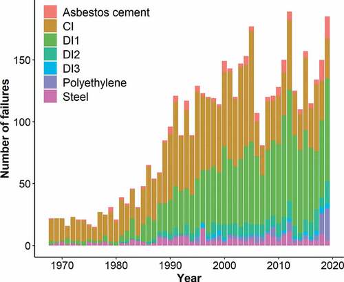
Figure 5 shows the number of annual failures per material type in the failure database. Failures occur largely in cast iron, DI1, and DI2. The share of ductile iron failures has continuously increased in the last few decades. Although low, failures for asbestos cement and PE have also been increasing in recent years, whereas steel pipe failures have been stable.

Figure 5. Annual recorded failures by material type.

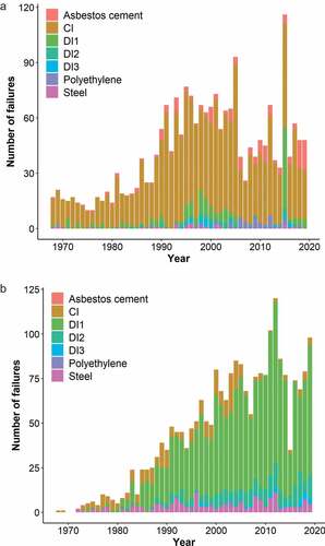
The reported cause of failure consisted of either rupture (i.e., large lengthwise or circumferential crack caused by soil movement), point (i.e., point leak caused by corrosion), excavation (i.e., accidental penetration of pipe during excavation works), joint (i.e., failure at pipe joint) or unknown. The accuracy of these recordings is unclear. Failures caused by multiple mechanisms (e.g., synergistic effect of corrosion and soil movement) are evidently possible but not mentioned. Nevertheless, this data is of interest and is explored below. The vast majority of failures were attributed to either soil movement or corrosion and are shown in Figure 6. There is a strong correlation between material and failure type for cast iron and ductile iron. This relationship has been documented in numerous studies (Infraguide, 2002; Makar et al., 2001; Balvant Rajani & Kleiner, 2001).

Figure 6. Annual recorded failures caused by (a) soil movement and (b) corrosion.

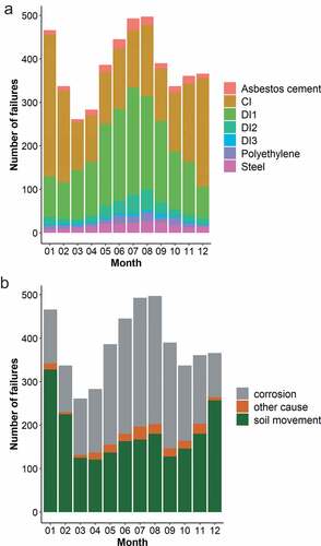
The seasonal effects on pipe failure have also been well documented by numerous water utilities and in published reports (Infraguide, 2002). Seasonal temperature changes cause soil movement, commonly referred to as frost heave, which leads to increased stress on pipes and often causes old cast iron pipes to break. Ductile iron pipes are more malleable and can better handle such stress fluctuations. This trend is visible in the failure data. Figure 7 contains the average monthly failures by material type and by failure type. Cast iron failures peak in December and January, and so do rupture failures. Corrosion-caused point failures and the corresponding number of ductile iron failures greatly increase in spring and summer when the moisture content of the soil is higher, which facilitates the redox reactions necessary for corrosion to take place.

Figure 7. Average monthly failures by (a) material type; (b) reported cause of failure.

3.2. Step 2: choose target and input parameters

The time until the next failure is chosen as the target value for the ANN because it is deemed to be the most useful for an infrastructure manager prioritizing short-term interventions. The parameter is calculated as the difference between failure year and installation year if a pipe had not previously failed and otherwise as the time between failures.

To correct the right-censored data for PE and DI3 pipes, values are randomly generated for the time to first failure. Failure is defined as observable, associated with a specific pipe, and requiring a corrective maintenance intervention. The Weibull distributions derived from the Scholten et al. (2013) study are used. The Weibull distribution is widely found in the pipe failure literature (Eisenbeis, 1994; Kimutai et al., 2015; Mailhot et al., 2000; Røstum, 2000; Scheidegger et al., 2015, 2013; Snider & McBean, 2019). Other predictive attributes (length, diameter, etc.) are not considered in order to match the granularity of the Scholten et al. (2013) priors. Scholten et al. (2013) derived the parameters by interviewing eight experts in Switzerland using a detailed expert elicitation protocol to obtain estimates of the survival quantiles of commonly occurring pipe materials (3^rd-generation cast iron, 1^st-generation ductile iron, steel, asbestos cement, and PE) at different ages. Experts were asked to provide a range of ages at which they expect a proportion of pipes to be replaced based on the technical service life of the material. The effect of coordination with other utilities or management strategies on pipe replacement was ignored in the interview. These estimates were then calibrated using data from the water utility of Lausanne, which is similar to the participating utility in terms of size, standards, operating practices, pipe suppliers, contractors, climate, elevation, and soil conditions. Figure 8 shows a comparison of the obtained Weibull distributions from Scholten et al. (2013) and the recorded failures of the utility from the case study.

Figure 8. Comparison of time to first failure of observations (histogram) and Weibull distribution (red curve) based on expert opinion for a) asbestos cement, b) steel, c) DI1.

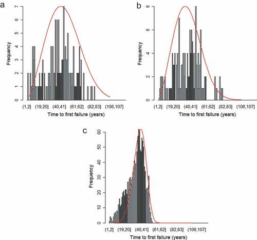
The Weibull distributions fit the recorded time to first failure distributions reasonably well for asbestos cement, steel and DI1. The Weibull parameters for PE are used to generate a time to first failure for PE and DI3 pipes, as DI3 was not included in the study. Wallerath and Wehr (2014) projected a similar service life for both PE and DI3 pipes. Thus, this assumption appears reasonable. Scholten et al. (2013) stated that the estimated parameters for PE were the most uncertain due to the lack of available data and limited experience experts had with PE failures. In other words, the estimates from the expert elicitation are acceptable for use in short-term failure prediction but must be regularly updated.

By adding generated failure data, noise is added to the complex relationships between inputs and output of the ANN model. This is counterbalanced by the resulting correction of right censorship. Thus, an important consideration is the ratio of generated failures to total failures used to train the ANN. This depends on the number of failure observations needed for a representative sample. In this study, a threshold ratio (i.e., pipes that have failed to total pipes) of 10% is chosen above which the recorded failures are deemed a representative sample. All pipe materials are above this threshold, except PE and DI3 (see Table 3). For PE and DI3 pipes, 708 failures and 192 failures are respectively generated for pipes that had not yet failed. These failures complemented the recorded failures of 125 unique PE and 45 DI3 pipes, to increase the percentage of pipes that had failed from 1.5% and 1.9% respectively to 10%. The Weibull probability density function is shown below (see Equation (3)). Figure 9(a) shows the comparison of observed time to first failure for PE pipes with the Weibull distribution obtained from Scholten et al. (2013) and Figure 9(b) the resulting histogram of actual and generated failures.

(3) $f(x)=\frac{k}{\lambda }{\left(\frac{x}{\lambda }\right)}^{k-1}{e}^{-{\left(\frac{x}{\lambda }\right)}^k}$(3)

Figure 9. Distribution of time to first failure of (a) PE failures in failure database with fitted Weibull distribution (k = 1.81, λ = 65.72); (b) resulting PE failures.

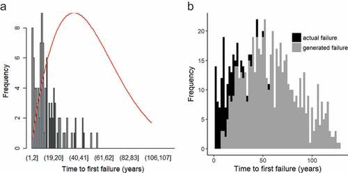
Where x is pipe age, k is the shape factor, and λ is the scale factor.

Input parameters are chosen after consulting the scientific literature and considering the available data. In addition to the studies listed in Table 1, Kabir (2016) provides an excellent overview of input parameters that have been used in published statistical failure prediction models. Table 5 contains the inputs chosen for the ANN models as well as the parameter ranges.

Table 5. ANN input and target parameters.

Parameter	Type	Units/Description	Training data
			Observed failures	Observed and generated failures
Total entries	Integer	Number of entries	4622	5522
Generated failures	Integer	Number of entries	0	708 (PE), 192 (DI3)
Previous failures	Integer		0–12	0–12
Diameter	Numeric	mm	30–600	30–600
Length	Numeric	m	0.4–1631.8	0.4–1631.8
Build year	Integer		1900–2019	1900–2019
Material	Binary	7 distinct categories (CI, DI1, DI2, DI3, ST, AC, PE)
Zoning	Binary	13 distinct categories based on use (e.g., residential, industrial) and population density
Soil texture	Binary	11 distinct categories based on clay, silt, sand composition
Time to failure	Numeric	Years	0–115	0–183

Categorical variables such as material and soil type are encoded using the one-hot encoding protocol. Previous failure prediction studies have developed material-specialized ANN models, but Kerwin et al. (2018) found comparable performance using a generalized ANN with material as an input. The soil classifications are made using the soil texture guidelines issued by the Soil Science Society of Switzerland (Switzerland, 2010). According to the web-based GIS shapefile, the soil samples were taken at a depth of between 2 and 20 cm and consisted of at least 10 samples per measurement. Eleven separate categories were defined. Soil characteristics affect soil movement throughout the year (e.g., frost and soil expansion loads) and the corrosive potential of the environment (chloride levels, moisture content, soil pH, etc.) (Liu et al., 2012).

Thirteen categories are used for zoning, based on land use (e.g., residential, industrial, recreational, downtown/village hub, etc.) and population density. Zoning is included to serve as a proxy for the level of vehicular traffic and the operating pressure of pipes in the area. High traffic loads exert stresses on buried pipes, which accelerates deterioration (Liu et al., 2012), and zoning is a good indicator of the required water supply. For example, dense urban areas have a higher water demand and taller buildings and thus require higher levels of pressure than rural areas (SVGW, 2012). The categories differed in use (e.g., residential, industrial, green space, etc.) and population density (e.g., high-density residential area, low-density residential area, etc.).

In this study, a data split of 80 – 10 – 10 is used between training, testing, and validation sets. Alternate approaches include determining the set of inputs that minimize the Akaike information criterion (Akaike, 1973) or Bayesian information criterion (Kabir et al., 2015b; Kimutai et al., 2015; Snider & McBean, 2019).

3.3. Step 3: develop ANN architecture

To determine the optimal number of nodes in the hidden layer, a double-looped process is used, where 25 different random initial weights are used for the increasing number of nodes in the hidden layer. Architectures up to 25 nodes are examined using MSE, resulting in 625 examined ANNs. The architecture with the lowest MSE is chosen. Implementation is done in MATLAB using the Neural Network Toolbox.

3.4. Step 4: compare scaling method, activation functions, and training algorithm

Next, the scaling method, activation functions, and training algorithm are altered to examine their effect on ANN performance. The scaling methods examined are min-max scaling (see Equation (4)(4) $Z_{i,min\mathrm{\_}max}=\frac{x_i-min(x)}{max(x)-min(x)}$(4) ) where data is rescaled using the minimum and the maximum value of the variable in a range of [0,1] or [−1,1] and standard deviation (z-score) normalization, where the mean value ($\bar{X}$) and the standard deviation (σ) is used to transform the data series to one with a mean value of 0 and a standard deviation of 1 (see Equation (5)(5) $Z_{i,std}=\frac{x_i-\bar{X}}{{\sigma }_X}$(5) ). Figure 10 shows that there is a negligible difference in results with the two methods. For all ANN models, standard deviation normalization is used.

(4) $Z_{i,min\mathrm{\_}max}=\frac{x_i-min(x)}{max(x)-min(x)}$(4)

(5) $Z_{i,std}=\frac{x_i-\bar{X}}{{\sigma }_X}$(5)

Figure 10. Investigation of the effect of training algorithm, scaling method and activation function on ANN model performance (scg – scaled conjugate gradient, lm: Levenberg-Marquardt).

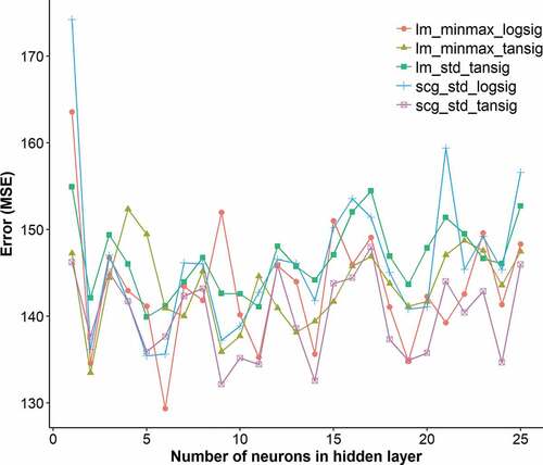
The activation functions examined are the hyperbolic tangent sigmoid transfer function, the log-sigmoid transfer. The linear transfer function is used as the second activation function for all instances.

Finally, the effects of two different backpropagation training algorithms (Levenberg-Marquardt, scaled conjugate gradient) were investigated. Levenberg-Marquardt uses the Jacobian of the performance function of the neural network, whereas the scaled conjugate gradient uses the derivative. The Levenberg-Marquardt algorithm usually requires the least amount of time but requires more memory (MATLABa, 2018), whereas the scaled conjugate gradient algorithm requires less memory and also provides good results depending on the problem and the data (MATLABb, 2018). Both methods use early stopping criteria for avoiding overfitting. Figure 10 shows the results of the performance comparison of the tested configurations (i.e., scaling, activation function, training algorithm) that performed best. The configuration composed of the scaled conjugate gradient algorithm with standard deviation scaling and the hyperbolic tangent activation function is chosen for reasons of speed and performance.

3.5. Step 5: evaluate model performance

Model performance is evaluated using MSE and the correlation coefficient. The regression scatterplots are shown for the ANN models in Figure 11. Overall and material-specific comparisons of the error histograms are shown in Figures 12–15. Table 7 contains the relative importance of the top 10 input parameters of both models. This is evaluated using the Connection Weight Approach, where the weights of the developed neural networks are used to compute the relative importance (RI) of each input (Olden & Jackson, 2002). The synaptic or connection weights of a neural network are the links between the inputs and the outputs. Larger weights indicate a link of greater importance. This approach has been found to more accurately estimate the input variable importance of ANN models compared to similar approaches (e.g., Garson’s Algorithm) (Olden et al., 2004). The relative importance is calculated using Equation (6)(6) $R{I}_i=\left|\sum _{h=1}^H{w}_{ih}{w}_h\right|$(6) , where w_ih is the weight between the i^th input parameter and hidden neuron h, and w_h is the weight between the hidden neuron h and the output.

(6) $R{I}_i=\left|\sum _{h=1}^H{w}_{ih}{w}_h\right|$(6)

Table 6. ANN model results.

Training data	Architecture	Dataset	Instances	MSE	R
Observed failures only	35 – 11 – 1	Training	3698	137.0	0.851
		Validation	462	138.8	0.812
		Testing	462	100.0	0.882
Observed and generated failures	35 – 9 – 1	Training	4418	343.6	0.732
		Validation	552	344.4	0.703
		Testing	552	250.1	0.794

Table 7. Input importance of ANN models (only top 10 inputs of both models shown).

Input	Trained with observed failures only			Trained with observed and generated failures
	Ranking	Weight	Relative	Ranking	Weight	Relative
Number of previous failures	1	2.90	100%	1	2.34	100%
Construction year	2	1.55	53%	2	1.00	43%
Soil – silt	3	0.60	21%	5	0.22	9%
Pipe material – DI1	4	0.48	17%	7	0.14	6%
Soil – clayey silt	5	0.39	14%	6	0.18	8%
Pipe material – DI2	6	0.33	11%	11	0.13	5%
Soil – silty clay	7	0.30	10%	10	0.13	5%
Zoning – urban/village hub	8	0.24	8%	18	0.06	3%
Zoning – high density downtown	9	0.19	7%	27	0.03	1%
Zoning – residential low density	10	0.19	6%	4	0.27	11%
Pipe material – PE	11	0.18	6%	3	0.61	26%
Pipe material – DI3	14	0.15	5%	8	0.14	6%
Soil – sandy silt	21	0.07	3%	9	0.14	6%

Figure 11. (a) Scatterplot for ANN only trained with observed failures. R = 0.851; (b) Scatterplot for ANN trained with observed and generated failures. R = 0.736.

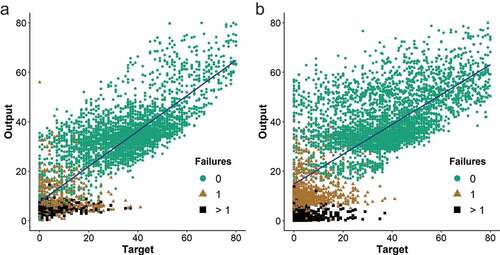
Figure 12. (a) Overall error histogram. MSE: 133.5 (ANN trained only with observed failures). MSE: 334.3 (ANN trained with observed and generated failures). (b) Error histogram for cast iron pipes. MSE: 186.2 (ANN trained only with observed failures). MSE: 204.5 (ANN trained with observed and generated failures).

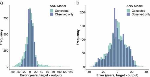
Figure 13. (a) Error histogram for DI1 pipes. MSE: 86.3 (ANN trained only with observed failures). MSE: 90.5 (ANN trained with observed and generated failures); (b) Error histogram for DI2 pipes. MSE: 94.8 (ANN trained only with observed failures). MSE: 92.9 (ANN trained with observed and generated failures).

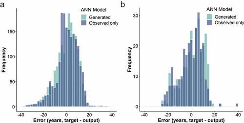
Figure 14. (a) Error histogram for DI3 pipes. MSE: 62.2 (ANN trained only with observed failures). MSE: 1260.9 (ANN trained with observed and generated failures); (b) Error histogram for PE pipes. MSE: 65.6 (ANN trained only with observed failures). MSE: 1070.9 (ANN trained with observed and generated failures).

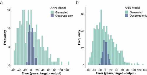
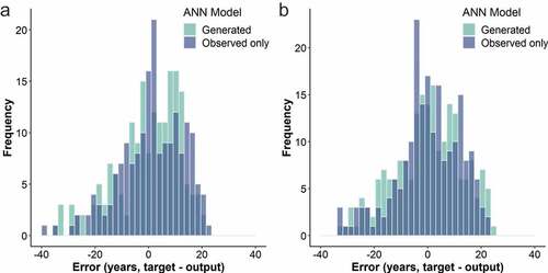
Figure 15. (a) Error histogram for asbestos cement pipes. MSE: 137.6 (ANN trained only with observed failures). MSE: 158.7 (ANN trained with observed and generated failures); (b) Error histogram for steel pipes. MSE: 142.8 (ANN trained only with observed failures). MSE: 173.1 (ANN trained with observed and generated failures).

4. Results

Table 6 summarizes the model configuration and performance of the developed ANN models for the three training phases. Figure 11 shows the error scatterplot and error histogram of the ANN models. Figures 12–15 contain the error histograms of both ANN models for the investigated pipe materials.

Table 7 shows the input importance of the two ANN models using the connected weights method. For brevity, only the inputs that are ranked in the top 10 of either model are shown.

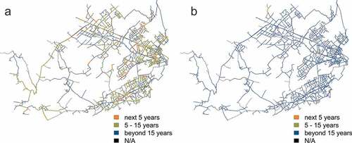
Figure 16 shows the results of time to next failure for pipes in the example subnetwork using the developed ANN models. Due to the uncertainty of the predictions, the following categories are used: failure expected in the next 5 years, 5–15 years, and beyond 15 years. Pipes that are not made of PE, cast iron, ductile iron, asbestos cement, or steel are shown in a thin black line (i.e., N/A) as no time to failure is calculated for these pipes.

Figure 16. Time to next failure (a) using ANN model trained with only observed failures; (b) using ANN model trained with observed and generated failures.

From Figures 11(a), 12(a) and Table 6, it is apparent that the ANN trained only with observed failures has a reasonable performance with a correlation coefficient of 0.882 and an obtained value of MSE of 100 in the testing phase of training. However, the resulting failure distributions for PE and DI3 in the case study (see Figures 16 and 17) are unreasonable due to the effects of right censorship. The addition of generated failures resulted in more reasonable failure estimates for PE and DI3, without significantly affecting the model performance for other materials. Overall, model performance decreased as expected, with the correlation coefficient dropping to 0.794 and the MSE increasing to 250.1 for the testing phase of training. By comparing the model performance by material subsets (see Figures 12–15), it is clear that the majority of error increase is limited to predictions for PE and DI3.

Figure 17. Distribution of time to next failure for example subnetwork for both developed ANN models for (a) PE pipes; (b) DI3 pipes.

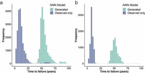
When applied to the case study subnetwork, there is a drastic difference observed between Figure 16(a and b) due to the high composition of PE and DI3 (28.0% and 8.3% respectively by length). Considering Figure 17, one can see that the addition of generated failures shifts the distributions of time to next failure by several decades for both PE and DI3. Based on the expectations of pipe manufacturers, industry publications, and the opinions of experts, the results of the ANN model trained with both observed and generated failures appear more reasonable and better suited for short-term intervention prioritization.

The influence of input parameters of the ANN models is analyzed using the connected weights approach. Table 7 shows that the most important input parameters in both models are the failure history followed by the construction year. This is in alignment with numerous other studies (Asnaashari et al., 2013; Christodoulou et al., 2003; Harvey et al., 2014; Lin & Yuan, 2019; Sattar et al., 2019; Snider & McBean, 2019). This influence can be clearly seen in the regression scatterplots of Figure 11, where the majority of the predicted failures in the range of 0 to 15 years had previously failed, and the majority of the predicted failures from 30 to 100 years had not. This relationship continues for pipes that have failed more than once, highlighting the negative correlation between the number of previous failures and the time to next failure. This relationship was also observed in Harvey et al. (2014).

Soil type, specifically whether the pipe was buried in an area with silty soil, and pipe material inputs are the next most important inputs for the ANN model trained only with observed failures. The soil classifications are made using the soil texture guidelines issued by the Soil Science Society of Switzerland (Switzerland, 2010). According to the web-based GIS shapefile, the soil samples were taken at a depth of between 2 and 20 cm and consisted of at least 10 samples per measurement. Ideally, these samples would have been taken deeper as water pipes are typically buried at depths of 1.2 to 1.5 m in Switzerland (SVGW, 2012), but it nonetheless provides a useful characterization.

The most important pipe material inputs are initially DI1 and DI2 (pipes with higher failure rates) but changed to PE and DI3 in the ANN model trained with generated and observed failures. The next important parameters are zoning-related, especially high-density areas or residential areas. This is unsurprising as the oldest pipes in this utility are mostly located in the high-density downtown area of the city, where the network first developed. This appears to indicate that inferential environmental attributes (soil type, zoning) are able to increase predictive performance.

Pipe length and diameter are not found to be important predictive inputs. Other studies have found the length to be an important predictor (Asnaashari et al., 2013; Kimutai et al., 2015; Winkler et al., 2018). In general, longer pipes are expected to have more failures, which is why length is used in normalizing failure statistics. In addition, one expects a higher probability of encountering sections with non-uniform bedding support (Hu & Hubble, 2007; Rajani & Tesfamariam, 2007), heavy traffic load (Liu et al., 2012), damage to corrosion protection layer, etc. Nonetheless, some studies have found the length to have a low predictive input (Harvey et al., 2014; Sattar et al., 2019) and Wang et al. (2009) found inconclusive evidence to suggest that longer pipes were more prone to failure than shorter pipes. Regarding diameter, several papers investigating pipe failures have observed that failure rate increased with smaller pipe diameter with the explanation that corrosion pits (Kettler & Goulter, 1985; Balvant Rajani & Makar, 2000) or chemical attack (Hu & Hubble, 2007) had a more significant structural effect on pipes with smaller diameters and thinner walls. In addition, the relationship between pipe diameter and failure mode has been well documented (Infraguide, 2002; Makar et al., 2001). Makar et al. (2001) described the relationship for cast iron pipes, writing that smaller diameter pipes are more susceptible to longitudinal bending failures while larger pipes are more likely to fail due to longitudinal cracking and bell shearing. Soil movement from clay swelling and shrinking was reported to be responsible for a large proportion of circumferential failures in small diameter mains in a study on asbestos cement pipes (Hu & Hubble, 2007). Nonetheless, other MLA failure prediction studies have also found that pipe diameter was less important than other inputs such as failure history, construction year and level of corrosion protection (Asnaashari et al., 2013; Harvey et al., 2014).

Evidently, there are notable differences between the weight distributions of the two ANN models (see Table 7). This is expected, as the addition of generated failures to the training data will inevitably have an effect. Although insights, such as node importance, can be gained by exploring the link weights, ANNs are referred to as black boxes. In other words, it is not possible to extract a precise mechanistic explanation to the optimized weight distribution nor explain changes that occur when generated failures are added to the training data.

Seasonal factors are not considered in the input parameters because the model output is years to next failure for individual pipes. Had the models been developed to predict the near future (i.e., upcoming weeks) network-wide failures, then seasonal parameters such as air and water temperature would have been considered. Several published models that considered shorter time horizons have included these parameters (See Table 1). Future work could involve considering the number of freeze-thaw cycles from historical temperature records to infer material fatigue. Other inputs are also imaginable, for instance, installation details such as the hired contractor, the pipe bedding and backfill material could be used to infer the quality of installation and other parameters that exert loads on buried pipes such as vehicular traffic, roadwork in the immediate vicinity, fluctuations in operating pressure and corrosive soils. Spatial failure characteristics could also be added. Goulter and Kazemi (1988) noted the spatial clustering of failure events in Winnipeg and Kimutai et al. (2015) made a similar observation for Calgary. Such information can be readily incorporated as an input into an MLA (Snider & McBean, 2018). The challenge, of course, is that much of this data was not recorded historically and is thus not available for analysis. Going forward, data collection of such parameters could help develop improved ANN failure prediction models.

5. Conclusion and outlook

The presented methodology is a systematic, iterative approach to the development of ANN failure prediction models to aid decision-makers in short-term prioritization. The performance of such models is influenced by a large number of factors, such as training data availability. One way to increase access to training data is to consider failures from all pipe materials and use them for training a generalized ANN, with pipe material modeled as a categorical input. Arguably, other attributes such as failure history and construction year are more relevant for failure prediction than pipe material. Such an approach allows newer materials with fewer failures to be included (PE and DI3). These materials often constitute significant portions of distribution networks and, of course, will ultimately surpass acceptable failure rate thresholds.

The development and use of preventive intervention strategies in infrastructure management (Adey, 2019) require predictions to be made on when failures are likely to occur. In the absence of sufficient data, it is justifiable to generate failures based on expert opinion. This approach has the disadvantage that the addition of generated failure data adds noise to the model; thus, the ratio of generated failures to total failures in the training dataset must be carefully considered. Ultimately, once sufficient data is available, such generated failures will be unnecessary. The alternative is a passive, reactive approach where infrastructure managers record failure events for several decades until sufficient data is available.

The example case study showed that the addition of generated failures improved short-term failure predictions for newer materials without significantly affecting the predictions of other materials. Model performance is explored by evaluating different ANN architectures and by comparing scaling techniques (i.e., min-max and standard deviation), activation functions (i.e., log-sigmoid and hyperbolic tangent sigmoid transfer function) and training algorithms (i.e., Levenberg-Marquardt, and scaled conjugate gradient). The overall performance is not significantly affected by changes to these three parameters. The best performing and most efficient combination are found to be the one using the standard deviation scaling, with the hyperbolic tangent sigmoid transfer function in conjunction with the scaled conjugate gradient error minimization training algorithm. The architecture and the initial weightings of links affected the model performance considerably more.

An area of future work is to improve the performance by modifying how the input parameters are fed into the ANN model. The analysis of input influence indicated the non-negligible contribution of soil type to model output. A more detailed consideration of soil properties will likely result in performance gains. Furthermore, several inputs had a surprisingly low contribution to the output, such as pipe diameter and length. Other studies have documented the relationship between these parameters and pipe failure, and thus it would be worthwhile to explore alternative ways of modeling these inputs. Moreover, operational parameters (e.g., pressure fluctuations, water quality parameters) are not investigated in this study and could be incorporated in future models.

Acknowledgments

The authors most gratefully acknowledge the water utility of Geneva (SIG) for providing the data for this study.

Disclosure statement

No potential conflict of interest was reported by the authors.

Additional information

Notes on contributors

Sean Kerwin

Sean Kerwin is a scientific assistant in the Infrastructure Management Group at the Institute of Construction and Infrastructure Management (IBI) of the ETH Zurich. His research focuses on intervention planning and asset management of water distribution networks.

Borja Garcia de Soto

Borja García de Soto is an Assistant Professor of Civil and Urban Engineering at New York University Abu Dhabi (NYUAD).

Bryan Adey

Prof. Dr. Bryan Adey is the Professor for Infrastructure Management at the Swiss Federal Institute of Technology in Zürich (ETHZ), Switzerland.

Kleio Sampatakaki

Kleio Sampatakaki and Hannes Heller are graduates of the Master's degree program in Civil Engineering at ETHZ. Ms. Sampatakaki is working as a structural engineer at the Gruner Wepf AG Zürich. Mr. Heller is working as a civil engineer at EBP.

References

- Achim, D., Ghotb, F., & McManus, K. (2007). Prediction of water pipe asset life using neural networks. Journal of Infrastructure Systems, 13(1), 26–30. doi:10.1061/(ASCE)1076-0342(2007)13:1(26)
- Adey, B. T. (2019). A road infrastructure asset management process: Gains in efficiency and effectiveness. Infrastructure Asset Management, 6(1), 2–14. doi:10.1680/jinam.17.00018
- Adey, B. T., Richmond, C., & García de Soto, B. (2017). Infrastructure management 2: Evaluation tools. ETH Zurich: Course script. Infrastructure Management.
- Ahn, J., Lee, S., Lee, G., & Koo, J. (2005). Predicting water pipe breaks using neural network. Water Science and Technology: Water Supply, 5(3–4), 159–172.
- Akaike, H. (1973). Maximum likelihood identification of Gaussian autoregressive moving average models. Biometrika, 60(2), 255–265. doi:10.1093/biomet/60.2.255
- Al-Barqawi, H., & Zayed, T. (2006). Condition rating model for underground infrastructure sustainable water mains. Journal of Performance of Constructed Facilities, 20(2), 126–135. doi:10.1061/(ASCE)0887-3828(2006)20:2(126)
- Allweyer, T. (2016). BPMN 2.0: Introduction to the standard for business process modeling, BoD-Books on Demand.
- Amaitik, N. M., & Amaitik, S. M. (2010). Prediction of pipe failures in water mains using artificial neural network models.
- Asnaashari, A., McBean, E. A., Gharabaghi, B., & Tutt, D. (2013). Forecasting watermain failure using artificial neural network modelling. Canadian Water Resources Journal, 38(1), 24–33. doi:10.1080/07011784.2013.774153
- Bishop, C. (2007). Pattern recognition and machine learning (Information Science and Statistics) (1st edn. 2006. corr. 2nd printing ed.). New York: Springer.
- Caradot, N., Riechel, M., Fesneau, M., Hernandez, N., Torres, A., Sonnenberg, H. & Rouault, P. (2018). Practical benchmarking of statistical and machine learning models for predicting the condition of sewer pipes in Berlin, Germany. Journal of Hydroinformatics, 20(5), 1131–1147. doi:10.2166/hydro.2018.217
- Castanedo, F. (2013). A review of data fusion techniques. The Scientific World Journal, 2013, 1–19. doi:10.1155/2013/704504
- Christodoulou, S., Aslani, P., & Vanrenterghem, A. (2003). A risk analysis framework for evaluating structural degradation of water mains in urban settings, using neurofuzzy systems and statistical modeling techniques. World Water & Environmental Resources Congress 2003. Reston, VA, USA: ASCE.
- Christodoulou, S., & Deligianni, A. (2010). A neurofuzzy decision framework for the management of water distribution networks. Water Resources Management, 24(1), 139–156. doi:10.1007/s11269-009-9441-2
- Cooke, R. (1991). Experts in uncertainty: Opinion and subjective probability in science. New York, New York: Oxford University Press.
- DVGW, W. (2006). 400-3: Technische Regeln Wasserverteilungsanlagen, Teil 3: Betrieb und Instandhaltung. Deutscher Verein des Gas-und Wasserfaches eV Bonn.
- Eisenbeis, P. (1994). Modelisation statistique de la prevision des defaillances des conduites d’eau potable (Doctoral Thesis. Strasbourg 1.
- Folkman, S. (2018). Water main break rates in the USA and Canada: A comprehensive study. Mechanical and Aerospace Engineering Faculty Publication. https://digitalcommons.usu.edu/mae_facpub/174
- García de Soto, B., Adey, B. T., & Fernando, D. (2014). A process for the development and evaluation of preliminary construction material quantity estimation models using backward elimination regression and neural networks. Journal of Cost Analysis and Parametrics, 7(3), 180–218. doi:10.1080/1941658X.2014.984880
- García de Soto, B., Adey, B. T., & Fernando, D. (2017). A hybrid methodology to estimate construction material quantities at an early project phase. International Journal of Construction Management, 17(3), 165–196. doi:10.1080/15623599.2016.1176727
- García de Soto, B., Bumbacher, A., Deublein, M., & Adey, B. T. (2018). Predicting road traffic accidents using artificial neural network models. Infrastructure Asset Management, 5(4), 1–13. doi: 10.1680/jinam.17.00028
- Geem, Z. W., Tseng, C.-L., Kim, J., & Bae, C. (2007). Trenchless water pipe condition assessment using artificial neural network. Pipelines 2007: Advances and Experiences with Trenchless Pipeline Projects, 1–9. https://ascelibrary.org/action/showCitFormats?doi=10.1061%2F40934%28252%2926
- Goulter, I. C., & Kazemi, A. (1988). Spatial and temporal groupings of water main pipe breakage in Winnipeg. Canadian Journal of Civil Engineering, 15(1), 91–97. doi:10.1139/l88-010
- Gressmann, M. (2020). PE-Rohrleitungen - seit Jahrzehnten bewährt. Aqua & Gas, 2020(3), 46–51.
- Grigg, N. S. (2009). National mains failure database project. Great Rivers: World Environmental and Water Resources Congress 2009.
- Harvey, R., McBean, E. A., & Gharabaghi, B. (2014). Predicting the timing of water main failure using artificial neural networks. Journal of Water Resources Planning and Management, 140(4), 425–434. doi:10.1061/(ASCE)WR.1943-5452.0000354
- Hessel, V. D. J. (2007). 100 Jahre Nutzungsdauer von Rohren aus Polyethylen. Rückblick und Perspektiven, 3R international, 46, 242–246.
- Hornik, K., Stinchcombe, M., & White, H. (1989). Multilayer feedforward networks are universal approximators. Neural Networks, 2(5), 359–366. doi:10.1016/0893-6080(89)90020-8
- Hu, Y., & Hubble, D. (2007). Factors contributing to the failure of asbestos cement water mains. Canadian Journal of Civil Engineering, 34(5), 608–621. doi:10.1139/l06-162
- Infraguide. (2002). Deterioration and inspection of water distribution systems. Ottawa, Canada: Federation of Canadian Municipalities and National Research Council.
- Jafar, R., Shahrour, I., & Juran, I. (2007). Modelling the structural degradation in water distribution systems using the artificial neural networks (ANN). Water Asset Management International, 3(3), 14–18.
- Jafar, R., Shahrour, I., & Juran, I. (2010). Application of Artificial Neural Networks (ANN) to model the failure of urban water mains. Mathematical and Computer Modelling, 51(9–10), 1170–1180. doi:10.1016/j.mcm.2009.12.033
- Kabir, G. (2016). Planning repair and replacement program for water mains: A Bayesian framework. Vancouver, Canada: University of British Columbia.
- Kabir, G., Demissie, G., Sadiq, R., & Tesfamariam, S. (2015a). Integrating failure prediction models for water mains: Bayesian belief network based data fusion. Knowledge-Based Systems, 85, 159–169. doi:10.1016/j.knosys.2015.05.002
- Kabir, G., Tesfamariam, S., Hemsing, J., & Sadiq, R. (2019). Handling incomplete and missing data in water network database using imputation methods. Sustainable and Resilient Infrastructure, 1–13. doi:10.1080/23789689.2019.1600960
- Kabir, G., Tesfamariam, S., Loeppky, J., & Sadiq, R. (2015b). Integrating Bayesian linear regression with ordered weighted averaging: Uncertainty analysis for predicting water main failures. ASCE-ASME Journal of Risk and Uncertainty in Engineering Systems, Part A: Civil Engineering, 1(3), 04015007. doi:10.1061/AJRUA6.0000820
- Kerwin, S., García de Soto, B., & Adey, T. B. (2018) Performance comparison for pipe failure prediction using artificial neural networks. Paper presented at the IALCCE 2018, Ghent, Belgium.
- Kettler, A., & Goulter, I. (1985). An analysis of pipe breakage in urban water distribution networks. Canadian Journal of Civil Engineering, 12(2), 286–293. doi:10.1139/l85-030
- Kimutai, E., Betrie, G., Brander, R., Sadiq, R., & Tesfamariam, S. (2015). Comparison of statistical models for predicting pipe failures: Illustrative example with the city of calgary water main failure. Journal of Pipeline Systems Engineering and Practice, 6(4), p 04015005. Retrieved from https://ascelibrary.org/doi/abs/10.1061/%28ASCE%29PS.1949-1204.0000196
- Kleiner, Y., Nafi, A., & Rajani, B. (2010). Planning renewal of water mains while considering deterioration, economies of scale and adjacent infrastructure. Water Science and Technology: Water Supply, 10(6), 897–906.
- Kleiner, Y., & Rajani, B. (2001). Comprehensive review of structural deterioration of water mains: Statistical models. Urban Water, 3(3), 131–150. doi:10.1016/S1462-0758(01)00033-4
- Kutyłowska, M. (2015). Neural network approach for failure rate prediction. Engineering Failure Analysis, 47, 41–48. doi:10.1016/j.engfailanal.2014.10.007
- Kutyłowska, M. (2017). Comparison of two types of artificial neural networks for predicting failure frequency of water conduits. Periodica Polytechnica Civil Engineering, 61(1), 1–6.
- Le Gat, Y., & Eisenbeis, P. (2000). Using maintenance records to forecast failures in water networks. Urban Water, 2(3), 173–181. doi:10.1016/S1462-0758(00)00057-1
- Lin, P., & Yuan, -X.-X. (2019). A two-time-scale point process model of water main breaks for infrastructure asset management. Water Research, 150, 296–309. doi:10.1016/j.watres.2018.11.066
- Liu, Z., Kleiner, Y., Rajani, B., Wang, L., & Condit, W. (2012). Condition assessment technologies for water transmission and distribution systems. United States Environmental Protection Agency (EPA), 108. https://cfpub.epa.gov/si/si_public_record_report.cfm?Lab=NRMRL&dirEntryId=241510
- Mailhot, A., Pelletier, G., Noël, J. F., & Villeneuve, J. P. (2000). Modeling the evolution of the structural state of water pipe networks with brief recorded pipe break histories: Methodology and application. Water Resources Research, 36(10), 3053–3062. doi:10.1029/2000WR900185
- Makar, J., Desnoyers, R., & McDonald, S. (2001). Failure modes and mechanisms in gray cast iron pipe. Underground Infrastructure Research, 1–10. https://nrc-publications.canada.ca/eng/view/object/?id=916578d5-55d7-4dde-8e8f-b480487bdb1c
- MATLAB. (2018). Neural network toolbox. Retrieved from https://ch.mathworks.com/de/products/neural-network.html.
- MATLABa. (2018). Matlab documentation, Levenberg-Marquardt backpropagation. Retrieved from https://ch.mathworks.com/help/nnet/ref/trainlm.html.
- MATLABb. (2018). Matlab documentation, Scaled conjugate gradient. Retrieved from https://ch.mathworks.com/help/nnet/ref/trainscg.html?searchHighlight=conjugate%20gradient&s_tid=doc_srchtitle.
- Mitchell, T. M., (1997). Machine Learning. New York, NY: Mcgraw-hill science. Engineering/Math, 1.
- Najafi, M., & Kulandaivel, G. (2005). Pipeline condition prediction using neural network models. Pipelines 2005: Optimizing Pipeline Design, Operations, and Maintenance in Today’s Economy, 767–781. https://ascelibrary.org/action/showCitFormats?doi=10.1061%2F40800%28180%2961
- Olden, J. D., & Jackson, D. A. (2002). Illuminating the “black box”: A randomization approach for understanding variable contributions in artificial neural networks. Ecological Modelling, 154(1–2), 135–150. doi:10.1016/S0304-3800(02)00064-9
- Olden, J. D., Joy, M. K., & Death, R. G. (2004). An accurate comparison of methods for quantifying variable importance in artificial neural networks using simulated data. Ecological Modelling, 178(3–4), 389–397. doi:10.1016/j.ecolmodel.2004.03.013
- Pelletier, G., Mailhot, A., & Villeneuve, J.-P. (2003). Modeling water pipe breaks—Three case studies. Journal of Water Resources Planning and Management, 129(2), 115–123. doi:10.1061/(ASCE)0733-9496(2003)129:2(115)
- Rajani, B., & Kleiner, Y. (2001). Comprehensive review of structural deterioration of water mains: Physically based models. Urban Water, 3(3), 151–164. doi:10.1016/S1462-0758(01)00032-2
- Rajani, B., & Makar, J. (2000). A methodology to estimate remaining service life of grey cast iron water mains. Canadian Journal of Civil Engineering, 27(6), 1259–1272. doi:10.1139/l00-073
- Rajani, B., & Tesfamariam, S. (2007). Estimating time to failure of cast-iron water mains. Proceedings of the Institution of Civil Engineers - Water Management, 160(2), 83–88. doi:10.1680/wama.2007.160.2.83
- Renaud, E., De Massiac, J., Bremond, B., & Laplaud, C. (2009). SIROCO, a decision support system for rehabilitation adapted for small and medium size water distribution companies. Strategic Asset Management of Water Supply and Wastewater Infrastructures, 329–344. London, UK: IWA Publishing.
- Rogers, P. D., & Grigg, N. S. (2009). Failure assessment modeling to prioritize water pipe renewal: Two case studies. Journal of Infrastructure Systems, 15(3), 162–171. Retrieved from https://ascelibrary.org/doi/abs/10.1061/%28ASCE%291076-0342%282009%2915%3A3%28162%29
- Røstum, J. (2000). Statistical modelling of pipe failures in water networks (Doctoral thesis). Norwegian University of Science and Technology.
- Sacluti, F. R. (1999). Modelling water distribution pipe failures using artificial neural networks. Edmonton, Canada: University of Alberta.
- Sattar, A. M., Ertuğrul, Ö. F., Gharabaghi, B., McBean, E. A., & Cao, J. (2019). Extreme learning machine model for water network management. Neural Computing & Applications, 31(1), 157–169. doi:10.1007/s00521-017-2987-7
- Scheidegger, A., Leitão, J. P., & Scholten, L. (2015). Statistical failure models for water distribution pipes–A review from a unified perspective. Water Research, 83, 237–247. doi:10.1016/j.watres.2015.06.027
- Scheidegger, A., Scholten, L., Maurer, M., & Reichert, P. (2013). Extension of pipe failure models to consider the absence of data from replaced pipes. Water Research, 47(11), 3696–3705. doi:10.1016/j.watres.2013.04.017
- Scholten, L., Scheidegger, A., Reichert, P., & Maurer, M. (2013). Combining expert knowledge and local data for improved service life modeling of water supply networks. Environmental Modelling and Software, 42, 1–16. doi:10.1016/j.envsoft.2012.11.013
- Shamir, U., & Howard, C. D. D. (1979). An analytic approach to scheduling pipe replacement. Journal - American Water Works Association, 71(5), 248–258. doi:10.1002/j.1551-8833.1979.tb04345.x
- Snider, B., & McBean, E. A. (2018). Improving time to failure predictions for water distribution systems using extreme gradient boosting algorithm. WDSA/CCWI Joint Conference Proceedings, Kingston, Ontario, Canada.
- Snider, B., & McBean, E. A. (2019). Improving urban water security through pipe-break prediction models: Machine learning or survival analysis. Journal of Environmental Engineering, 146(3), 04019129. doi:10.1061/(ASCE)EE.1943-7870.0001657
- SVGW. (2012). Standard on water distribution (W4) Part 4: Operation and maintenance.
- SVGW. (2014). Statistische Erhebungen der Wasserversorgungen in der Schweiz Betriebsjahr 2013. Zürich.
- SVGW. (2015a). Branchenbericht des schweizerischen Wasserversorgung. Zürich.
- SVGW. (2015b). Statistische Erhebungen der Wasserversorgungen in der Schweiz Betriebsjahr 2014. Zürich.
- SVGW. (2016). Statistische Erhebungen der Wasserversorgungen in der Schweiz Betriebsjahr 2015. Zürich.
- SVGW. (2017). Statistische Erhebungen der Wasserversorgungen in der Schweiz Betriebsjahr 2016. Zürich.
- SVGW. (2018). Statistische Erhebungen der Wasserversorgungen in der Schweiz Betriebsjahr 2017. Zürich.
- SVGW. (2019). Statistische Erhebungen der Wasserversorgungen in der Schweiz Betriebsjahr 2018. Zürich.
- Switzerland, S. S. S. O. (2010). Soil classification in Switzerland. Switzerland: Soil Science Society of Switzerland. Retrieved from http://www.soil.ch/cms/fr/publications/classification/
- Tabesh, M., Soltani, J., Farmani, R., & Savic, D. (2009). Assessing pipe failure rate and mechanical reliability of water distribution networks using data-driven modeling. Journal of Hydroinformatics, 11(1), 1–17. Retrieved from http://jh.iwaponline.com/content/ppiwajhydro/11/1/1.full.pdf
- Tscheikner-Gratl, F., Caradot, N., Cherqui, F., Leitão, J. P., Ahmadi, M., Langeveld, J. G., & Rodríguez, J. P. (2019). Sewer asset management–state of the art and research needs. Urban Water Journal, 16(9), 662–675. doi:10.1080/1573062X.2020.1713382
- Tversky, A., & Kahneman, D. (1974). Judgment under uncertainty: Heuristics and biases. Science, 185(4157), 1124–1131. doi:10.1126/science.185.4157.1124
- van Riel, W., Langeveld, J., Herder, P., & Clemens, F. (2017). The influence of information quality on decision-making for networked infrastructure management. Structure and Infrastructure Engineering, 13(6), 696–708. doi:10.1080/15732479.2016.1187633
- van Riel, W., van Bueren, E., Langeveld, J., Herder, P., & Clemens, F. (2016). Decision-making for sewer asset management: Theory and practice. Urban Water Journal, 13(1), 57–68. doi:10.1080/1573062X.2015.1011667
- vonRoll. (2020). Pipes and fittings. Retrieved from https://www.vonroll-hydro.world/files/content/downloads/Broschueren/rohre-und-formstuecke/ecopur/191007_vonRoll_ECOPUR_EN.pdf.
- Wallerath, M., & Wehr, R. (2014). Neubestimmung der technischen Nutzungsdauer von Rohrleitungen. DVGW energie: wasser-praxis, 7/8, 30–36.
- Wang, Y., Moselhi, O., & Zayed, T. (2009). Study of the suitability of existing deterioration models for water mains. Journal of Performance of Constructed Facilities, 23(1), 47–54. doi:10.1061/(ASCE)0887-3828(2009)23:1(47)
- Wilson, D., Filion, Y., & Moore, I. (2017). State-of-the-art review of water pipe failure prediction models and applicability to large-diameter mains. Urban Water Journal, 14(2), 173–184. doi:10.1080/1573062X.2015.1080848
- Winkler, D., Haltmeier, M., Kleidorfer, M., Rauch, W., & Tscheikner-Gratl, F. (2018). Pipe failure modelling for water distribution networks using boosted decision trees. Structure and Infrastructure Engineering, 14(10), 1402–1411. doi:10.1080/15732479.2018.1443145
- Wüst, J., Wenzel, M., Scholten, F., Wolters, M., Heinemann, J., & Bockenheimer, A. (2010). Integrität von PE-Gas-und Wasserleitungen der ersten Generation. 3 R International: zeitschrift fuer die Rohrleitungspraxis, 49(10), 534.
- Yuan, -X.-X. (2016). Principles and guidelines of deterioration modelling for water and waste water assets. Infrastructure Asset Management, 4(1), 19–35. doi:10.1680/jinam.16.00017