Geospatial Analysis of Alaskan Lakes Indicates Wetland Fraction and Surface Water Area Are Useful Predictors of Methane Ebullition

Abstract

Arctic-boreal lakes emit methane (CH₄), a powerful greenhouse gas. Recent studies suggest ebullition might be a dominant methane emission pathway in lakes but its drivers are poorly understood. Various predictors of lake methane ebullition have been proposed but are challenging to evaluate owing to different geographical characteristics, field locations, and sample densities. Here we compare large geospatial data sets of lake area, lake perimeter, permafrost, land cover, temperature, soil organic carbon content, depth, and greenness with remotely sensed methane ebullition estimates for 5,143 Alaskan lakes. We find that lake wetland fraction (LWF), a measure of lake wetland and littoral zone area, is a leading predictor of methane ebullition (adj. R² = 0.211), followed by lake surface area (adj. R² = 0.201). LWF is inversely correlated with lake area, thus higher wetland fraction in smaller lakes might explain a commonly cited inverse relationship between lake area and methane ebullition. Lake perimeter (adj. R² = 0.176) and temperature (adj. R² = 0.157) are moderate predictors of lake ebullition, and soil organic carbon content, permafrost, lake depth, and greenness are weak predictors. The low adjusted R² values are typical and informative for methane attribution studies. Our leading model, which uses lake area, temperature, and LWF (adj. R² = 0.325, n = 5,130) performs slightly better than leading multivariate models from similar studies. Our results suggest landscape-scale geospatial analyses can complement smaller field studies, for attributing Arctic-boreal lake methane emissions to readily available environmental variables.

北极湖泊释放一种强力温室气体——甲烷(CH4)。近来的研究表明, 冒泡可能是湖泊释放甲烷的主要途径, 但我们并不了解其驱动因素。由于地理特征、位置和样本密度的不同, 难以对现有的湖泊甲烷冒泡预测因子进行评估。我们将湖泊面积、湖泊周长、永久冻土、土地覆盖、温度、土壤有机碳含量、深度和绿度等地理大数据集, 与5,143个美国阿拉斯加湖泊的甲烷冒泡遥感估算, 进行了对比。将湖泊湿地比例(LWF)作为湖泊湿地和湖滨面积的衡量指标。我们发现, LWF是甲烷冒泡的主要预测因子(校正R2 = 0.211), 其次是湖面面积(校正R2 = 0.201)。LWF与湖泊面积呈负相关。因此, 面积小而湿地比例高的湖泊, 可能解释湖泊面积与甲烷冒泡之间的反比关系。湖泊周长(校正R2 = 0.176)和温度(校正R2 = 0.157)是湖泊冒泡的中等预测因子。土壤有机碳含量、永久冻土、湖泊深度和绿度是弱预测因子。在甲烷形成的研究中, 虽然校正R2值一般都较低, 但仍然提供了有用的信息。我们的模型采用了湖泊面积、温度和LWF(校正R2 = 0.325, n = 5,130), 略优于类似研究的多变量模型。研究结果表明, 为了将北极湖泊释放甲烷归因于现有的环境变量, 景观尺度的地理分析可以完善小区域研究。

Los lagos boreales del Ártico emiten metano (CH₄), un potente gas de efecto invernadero. Los estudios recientes sugieren que la ebullición podría ser una vía dominante en las emisión de metano en estos lagos, aunque sus causas siguen siendo pobremente comprendidas. Se han propuesto varios predictores sobre la ebullición del metano lacustre, pero su evaluación se dificulta por las diferentes características geográficas, ubicaciones y densidades de muestreo. En este artículo comparamos amplios conjuntos de datos geoespaciales sobre área lacustre, perímetro del lago, permafrost, cobertura del suelo, temperatura, contenido de carbón orgánico del suelo, profundidad y verdor, por medio de estimaciones de ebullición de metano, obtenidas por teledetección en 5.143 lagos de Alaska. Hallamos que la fracción de humedal lacustre (LWF), una medida del humedal lacustre y del área de la zona litoral, es un predictor principal de la ebullición del metano (adj. R² = 0.211), seguido por el área superficial del lago (adj. R² = 0,201). La LWF está inversamente correlacionada con el área del lago, por lo que una mayor fracción de humedal en los lagos más pequeños podría explicar una relación inversa comúnmente citada entre el área del lago y la ebullición del metano. El perímetro del lago (adj. R² = 0,176) y la temperatura (adj. R² = 0,157) son predictores moderados de la ebullición del lago, y el contenido de carbón orgánico del suelo, la permafrost, profundidad del lago y el verdor son predictores débiles. Los bajos valores R² ajustados son típicos e informativos para los estudios de atribución de metano. Nuestro modelo principal, que usa área del lago, temperatura y LWF (adj. R² = 0.325, n = 5,130) funciona ligeramente mejor que los principales modelos multivariados de estudios similares. Nuestros resultados sugieren que los análisis geoespaciales a escala de paisaje pueden complementar estudios de campo más pequeños, para atribuir las emisiones de metano de los lagos boreales del Ártico a variables ambientales fácilmente disponibles.

Key Words:

• Arctic-boreal lakes
• geospatial analysis
• methane emissions
• spatial regression
• upscaling

关键词:

• 北极湖泊
• 地理分析
• 甲烷排放
• 空间回归
• 升尺度

Palabras clave:

• análisis geoespacial
• emisiones de metano
• escalado
• lagos boreales del Ártico
• regresión espacial

Northern lakes are a major source of methane (CH₄), an important greenhouse gas shaping current and future climate change projections (Walter, Smith, and Chapin 2007; Arctic Monitoring and Assessment Programme 2015; Dhakal et al. 2022). Currently, the global methane budget is estimated as +551 to 737 Tg CH₄ yr⁻¹ (Saunois et al. 2020; Lu et al. 2021), with northern high-latitude lakes, wetlands, and coastal waters contributing ∼15 to 112 Tg CH₄ yr⁻¹ (McGuire et al. 2009; Bastviken et al. 2011; Arctic Monitoring and Assessment Programme 2015). High-latitude lakes and ponds account for ∼2.4 to 17.7 Tg CH₄ yr⁻¹ (Wik et al. 2016; Matthews et al. 2020; Saunois et al. 2020) despite occupying just 6 percent of northern landscapes (Olefeldt et al. 2021), thus comprising a particularly potent source of methane to the atmosphere. The Arctic is being affected by climate change at a rate nearly four times higher than the rest of the world, thus a better understanding of global methane emissions is particularly important for these regions (Rantanen et al. 2022).

Knowledge of total lake emissions is limited by sparse spatial sampling of the world’s lakes, however, with the largest field data syntheses comprising just 561, 1,247, and 575 lakes, respectively (DelSontro et al. 2019; M. Kuhn et al. 2021; Johnson et al. 2022). Due to the spatial heterogeneity of emissions, interpolation techniques are not sufficient for broad-scale estimates, so regression (Bastviken et al. 2004; Engram et al. 2020; Deemer and Holgerson 2021; M. Kuhn et al. 2021) and machine learning (Ludwig et al. 2022) are predominantly used. Lake methane emissions occur through four major pathways: diffusion from the water surface to the air (diffusive flux), release of bubbles from the sediment (ebullitive flux), release from sediment to the air through vegetation (plant-mediated flux), and release of dissolved methane buildup during ice melt (storage flux; Bastviken et al. 2011; Sanches et al. 2019). Diffusive flux is the best studied of these pathways, due to a relative ease of measurements and more homogeneous production throughout a lake and over time. Even so, numerous studies indicate that ebullition might be the dominant emission pathway, with plant-mediated and storage fluxes accounting for only a small fraction of emissions (Walter, Smith, and Chapin 2007; Bastviken et al. 2011; DelSontro et al. 2016; Wik et al. 2016). Upscaled calculations of global methane emissions based only on diffusive flux therefore underestimate total lake CH₄ flux, perhaps by as much as 277 percent (Sanches et al. 2019). Improved understanding of the drivers and spatial variability of lake ebullition processes is needed, particularly over landscape scales.

Many detailed, fine-scale ebullition regression studies report lake area (e.g., Bastviken et al. 2004; Sepulveda-Jauregui et al. 2015), temperature (air, water, and sediment temperature are inherently correlated and thus variously used; e.g., DelSontro et al. 2016; Praetzel, Schmiedeskamp, and Knorr 2021), and trophic status (e.g., Sepulveda-Jauregui et al. 2015; Zhou et al. 2020; Praetzel, Schmiedeskamp, and Knorr 2021) to be leading predictor variables (Table S.1 in the Supplemental Material). Lake area is often inversely proportional to CH₄ ebullition, with smaller lakes emitting more methane per unit area than large lakes; these correlations can have adjusted R² as high as 0.78 (n = 17; Bastviken et al. 2004). Trophic status, a measure of biological productivity, is considered a significant factor in methane emissions with highly productive waters having higher emissions (Zhou et al. 2020). Bastviken et al. (2004) found that a model using both lake area and total phosphorus (TP, a measure of trophic status) is best for predicting methane ebullition for thirteen lakes in North America and Eurasia (adj. R² = 0.89), and DelSontro et al. (2016) found that a model using TP and sediment temperature is best for predicting ebullition (adj. R² = 0.52) for thirteen lakes and ponds in Québec. Praetzel, Schmiedeskamp, and Knorr (2021) found that temperature is a strong individual predictor (R² = 0.53, n = 195), and a model combining temperature, porosity, and organic carbon is the best overall predictor (R² = 0.68, n = 193). Organic carbon availability in the form of soil organic carbon (SOC) and dissolved organic carbon (DOC) is also an important factor in CH₄ production and emissions (e.g., Negandhi et al. 2013; Walter Anthony et al. 2021). Depth also has a strong effect on ebullition, with shallower lakes having higher ebullitive fluxes than deeper lakes (e.g., DelSontro et al. 2016; Wik et al. 2018; G. Wang et al. 2021). Additional variables such as permafrost presence (e.g., Walter Anthony et al. 2021) and littoral (shallow or vegetated) zone area (e.g., Juutinen et al. 2003; Wik et al. 2018) have also been found to be statistically significant at a regional scale. In general, all regression studies typically yield low R² values, due to the inherent stochasticity of methane ebullition, but these finer scale, field-based studies tend to have higher predictive power (e.g., R² > 0.5).

Broad-scale ebullition regression studies similarly find lake area (e.g., Engram et al. 2020; Deemer and Holgerson 2021; M. Kuhn et al. 2021), temperature (e.g., Aben et al. 2017; Sanches et al. 2019; Deemer and Holgerson 2021), and trophic status (e.g., Yvon-Durocher et al. 2014; DelSontro, Beaulieu, and Downing 2019; Deemer and Holgerson 2021) to be leading predictors but with significantly lower correlation coefficients (Table S.1). Lake area is readily obtained from remote sensing (e.g., Smith et al. 2005; Messager et al. 2016; Muster et al. 2017; Cooley et al. 2019; Kyzivat et al. 2019; Kyzivat et al. 2022), making it a frequent variable in studies with broad spatial domains. M. Kuhn et al. (2021) found that ebullitive fluxes from seventy lakes are best predicted by a model using lake area alone (adj. R² = 0.21). As with area, trophic status can be estimated from remotely sensed “greenness” or chlorophyll-a (e.g., C. Kuhn and Butman 2021; M. Kuhn et al. 2021). Using individual regression models, DelSontro, Beaulieu, and Downing (2019) found chlorophyll-a to be the best of four predictors of methane ebullition (R² = 0.317, n = 65), and Deemer and Holgerson (2021) found a multiple regression model combining water-body type, latitude, chlorophyll-a, and lake area to be the best predictor of methane ebullition (R² = 0.29, n = 130). Although not quite as strong a predictor as area and trophic status, temperature is also frequently cited with R² = 0.1 (n = 110; Deemer and Holgerson 2021) and adj. R² = 0.06 (n = 68; M. Kuhn et al. 2021). Wik et al. (2016) suggested that temperature is a driving factor in lake methane ebullition only if there is sufficient organic carbon available for CH₄ production. Organic carbon in the form of DOC is also cited as a leading predictor by M. Kuhn et al. (2021; adj. R² = 0.14, n = 72). As with the regional studies, depth (e.g., Wik et al. 2016; Deemer and Holgerson 2021), permafrost presence (e.g., Wik et al. 2016; M. Kuhn et al. 2021), and littoral zone (near-shore zone shallow enough for aquatic vegetation) area (e.g., Sanches et al. 2019; Kyzivat et al. 2022) are cited as additional predictors. These types of studies with much broader spatial domains and often coarser resolution typically yield R² < 0.30 for sample sizes larger than 100.

It is challenging to compare the relative importance of environmental predictor variables spanning different studies, time scales, and geographic areas (Julian et al. 2013). As explained by Julian et al. (2013), most studies are conducted in specific regions or over short time scales, which limits understanding of broad-scale phenomena. Negandhi et al. (2013) and DelSontro et al. (2016), for example, considered few lakes but their studies were detailed and field-intensive, including such variables as depth, DOC, chlorophyll concentration, and sediment temperature. Alternatively, broad-scale studies often examine thousands of lakes with few variables (e.g., DelSontro, Beaulieu, and Downing 2019), or lakes in aggregate only (e.g., Kohnert et al. 2018). M. Kuhn et al. (2021) struck a balance between these two extremes by considering up to twenty variables for 1,247 Arctic-boreal lakes and ponds in one of the largest synthesis studies to date. Ebullitive flux data, however, are available for only 175 of these 1,247 lakes and ponds. Limited ebullition measurements are a commonly cited shortcoming of global CH₄ modeling efforts (Sanches et al. 2019). Furthermore, the relevance of predictor variables across spatiotemporal scale has yet to be evaluated. Thus, to accurately predict ebullition, a trade-off exists between more powerful field studies and more spatially inclusive synthesis studies.

A new data set for 5,143 Alaska lakes (Engram, Walter Anthony, and Meyer 2020) has vastly increased observations of landscape-scale variation in methane ebullition and provides an opportunity to test the importance of environmental predictors of lake methane ebullition at a common spatial scale. Here, we use individual and multiple linear regression, as in previous studies (e.g., DelSontro, Beaulieu, and Downing 2019; Deemer and Holgerson 2021; M. Kuhn et al. 2021; Table S.1), to examine correlations between this novel lake ebullition product and widely available environmental variables. Lake area, temperature, and trophic status are commonly used in the literature as predictors for upscaling emissions, but the rationale of including them might be based on convenience or location-specific field studies. By adding a variety of other potential predictor variables typically assessed at different spatial and temporal scales, we aim to determine the best predictors of mean annual methane ebullition at the pan-Arctic scale. Identifying and ranking drivers of ebullition would allow landscape-scale geospatial analyses to be better integrated with smaller field studies and would highlight important remote sensing and geographic information systems (GIS) variables to use in the absence of field data (e.g., at the global scale). Alternatively, a lack of improvement to the typical R² values from previous regression studies would imply there are important unmeasured variables still needed to allow these broad-scale predictions. In addition to ranking variables, we seek the best and most parsimonious predictive model from the variables that we have compiled. This analysis aims to inform future estimates of methane emissions from Arctic-boreal lakes through statistical upscaling or machine learning.

Data and Methods

Our study area was determined by the spatial domain of the methane ebullitive flux data set of Engram, Walter Anthony, and Meyer (2020), which contains ebullitive fluxes for 5,143 lakes in five dispersed regions of Alaska: Atqasuk, Barrow (now known as Utqiaġvik), Fairbanks, Seward Peninsula, and Toolik regions (Figure 1). Thus, our study area and regions are identical to those from Engram et al. (2020). Mean annual air temperature varies from −10 °C in Barrow to −4 °C in Fairbanks (Table 1). All regions fall within the continuous permafrost zone, except for Fairbanks, where permafrost thaw is widespread. Thermokarst lakes, which form in depressions caused by thawing permafrost and have the greatest emissions in organic-rich yedoma soils, are present in Atqasuk (non-yedoma), Barrow (non-yedoma), Seward Peninsula (yedoma), and Fairbanks (yedoma). Fairbanks also has anthropogenic gravel pit lakes as well as Tanana River floodplain lakes, whereas the lakes in Toolik are glacial lakes (Table 1). Together, these five regions represent a variety of lake types found in Alaska and across the Arctic and sub-Arctic.

Figure 1. Remotely sensed wintertime methane ebullition flux (g CH₄ m⁻²yr⁻¹) for 5,143 Alaskan lakes as estimated by Engram, Walter Anthony, and Meyer (2020) for five study regions: (A) Atqasuk, (B) Barrow Peninsula, (C) Fairbanks, (D) Seward Peninsula, and (E) Toolik.

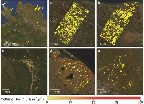
Table 1. Study site characteristics and ebullitive fluxes

Region	Lake types	Permafrost	MAAT (˚C)	n	M lake area ± SD (km^2)	M ebullitive flux (mg m^−2 d^−1 lake^−1)	Total ebullitive flux (mg m^−2 d^−1)
Atqasuk	Thermokarst (non-yedoma)	Continuous	−9.8	2,397	0.15 ± 0.47	1.32 ± 2.29	3,160
Barrow	Thermokarst (non-yedoma)	Continuous	−10.3	1,448	0.33 ± 2.02	3.62 ± 3.17	5,239
Fairbanks	Thermokarst (yedoma), anthropogenic gravel pit, Tanana River floodplain	Discontinuous	−4.0	178	0.04 ± 0.07	17.3 ± 24.0	3,085
Seward	Thermokarst (yedoma)	Continuous	−6.5	629	0.08 ± 0.21	10.9 ± 10.1	6,884
Toolik	Glacial	Continuous	−9.0	491	0.05 ± 0.11	5.50 ± 6.95	2,702

Note: MAAT = mean annual air temperature.

This methane data product was derived from satellite synthetic aperture radar (SAR), an active remote sensing in which microwave radiation is reflected off the earth’s surface and the timing of its return is used to construct a rasterized image. The phase and amplitude of the radar return can be used to determine the types of surfaces the waves interacted with (Smith 2002). SAR data can be obtained in the dark as well as through cloud cover (Engram et al. 2013), a useful benefit in the Arctic where there is little sunlight during the winter.

Engram et al. (2020) obtained SAR backscatter data over lakes from the Phased Array type L-band Synthetic Aperture Radar (PALSAR) instrument on the Advanced Land Observing Satellite (ALOS-1) satellite. An annual ebullitive flux was derived for each lake using the relationship between wintertime backscatter from rough surfaces created by methane bubbles trapped in ice and measurements from year-round, semiautomated bubble traps submerged in a subset of lakes within each region. The resulting data set includes lakes ranging from 0.00345 km² to 58.1 km² in area with a mean area of 0.176 km² and standard deviation of 1.13 km², each with a mean annual ebullition estimate over the years 2007 to 2010.

Geospatial data sets of lake morphometry, climate, depth, SOC, greenness, land cover, and permafrost were compiled from various sources (Table 2, Table S.2). Lake areas and perimeters were obtained from the lake polygons provided by Engram, Walter Anthony, and Meyer (2020). Climate variables come from the NASA Daymet product, which provides daily 1-km gridded estimates of temperature, precipitation, vapor pressure, and other variables, informed by daily meteorological observations (Thornton et al. 2020). Lake depth estimates, modeled lake area, and surrounding topography were obtained from the HydroLAKES vector database, which is available for lakes 10 ha (0.1 km²) in area and larger (Messager et al. 2016). SOC estimates, based on interpolated field observations, were obtained at 250 m resolution for six depth intervals between 0 and 200 cm (Poggio et al. 2021). Summer lake greenness data, estimated for 1,063 Alaskan lakes from the HydroLAKES database using Landsat imagery, were obtained from C. Kuhn and Butman (2021). Owing to a 10-ha minimum lake area requirement in both the greenness and depth products, there are only 965 lakes for which both predictor variables are available. Annual Landsat-derived land-cover maps spanning the NASA Arctic-Boreal Vulnerability Experiment (ABoVE) spatial domain at 30 m spatial resolution were obtained from J. A. Wang et al. (2019) and include six terrestrial classes (evergreen forest, deciduous forest, shrubland, herbaceous, sparsely vegetated, barren), three wetland classes (fen, bog, shallows/littoral), and one water class. This data set was not developed for purposes of wetland mapping and thus excludes certain wetland subcategories, such as forested wetlands, marshes, and shallow open-water wetlands. Based on inspection, the shallows/littoral class is rarer than expected for these shallow arctic lakes (area-weighted average = 25 percent of buffered lakes), suggesting that this wetland class underreports true shallow or littoral areas. Nevertheless, this land-cover map was developed for an overlapping Arctic-boreal domain and has an appropriate resolution to compare with the ebullition data so is included in our analysis. Near-surface (1-m) permafrost probability estimates were obtained at 30 m resolution from Pastick et al. (2015).

Table 2. Selected representative variables with sources, variable descriptions, shorthand variable names, data formats, and spatial resolutions

Source	Variable description	Variable name	Data format	Resolution	n
Engram, Walter Anthony, and Meyer (2020)	Region (Atqasuk, Barrow, Fairbanks, Seward, or Toolik)	Region	Categorical	0.005 km^2	5,143
	Methane ebullition flux (mg m^−2 d^−1)	MassFlxCH4	Vector	0.005 km^2	5,143
	Lake area (km^2)	AreaSqkm
Derived from Engram, Walter Anthony, and Meyer (2020)	Lake perimeter (km)	Perimeter	Tabular	0.005 km^2	5,143
Messager et al. (2016)	Lake depth (m)	Depth_avg	Vector	0.1 km^2	1,224
Pastick et al. (2015)	Mean permafrost probability within 1 m of the surface	Pfrst_mean	Raster	30 m	5,143
J. A. Wang et al. (2019)	Fraction of combined wetland class (LWF) in lake and surrounding wetlands within 100 m of lake	lbf_100n	Raster	30 m	5,139
Thornton et al. (2020)	Average winter temperature (˚C)	Tavg_W	Raster	1 km	5,141
Poggio et al. (2021)	Soil organic carbon content in the fine earth fraction (dg/kg)	SOC	Raster	250 m	5,130
C. Kuhn and Butman (2021)	Mean Landsat growing season surface reflectance (Rs) in the green wavelengths	Greenness	Tabular	0.1 km^2	1,061

Note. An expanded version of this table presenting all compiled variables is available in the Supplemental Materials (Table S.2).

Geospatial data sets were compiled and reprojected to a common equal-area reference system in ArcGIS Pro 2.8.3 for comparison with the lake ebullitive flux data. Each variable from Daymet was extracted to a separate raster using the Make NetCDF Raster Layer, then the Mosaic to New Raster tool was used to merge the tiles for each variable into a single raster for ease of processing. NoData values were removed from the permafrost probability raster, leaving all values ranging from 0 to 100. The SoilGrids raster was clipped to the extent of Alaska and each band, representing a unique variable for the 0 to 5-cm depth interval, extracted as a new raster. All data sets were reprojected to the Alaska Albers Equal Area Conic projection (EPSG:3338). Finally, these data sets were spatially joined to the original shapefile of Engram, Walter Anthony, and Meyer (2020) to enable comparisons with their methane ebullition data.

Lake perimeters were calculated from lake polygons of Engram, Walter Anthony, and Meyer (2020) using the Calculate Geometry tool in ArcGIS Pro 2.8.3, and the Field Calculator tool used to calculate perimeter-to-area (P/A) ratios. A unique identifier (LAKEID) was created for each lake, and the Zonal Statistics as Table tool was used for each of the raster layers (except land-cover variables, which are described next) to extract the mean raster values within each lake polygon. The LAKEIDs were then used to join these attribute tables containing information on permafrost, climate, and SOC to the original lake polygons. Where available, the vector data sets for lake depth and greenness were also spatially joined to the updated shapefile. Lake areas were already included as attribute information in Engram, Walter Anthony, and Meyer (2020).

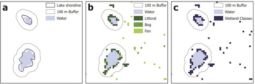
Land-cover data of J. A. Wang et al. (2019) were processed differently for terrestrial and wetland classes due to their different frequencies and clustering in the landscape. First, land-cover data were extracted and clipped to the extent of Alaska, and binary true–false (1–0) rasters were created for each of the ten land-cover variables. Lake polygons of Engram et al. (2020) were buffered outward by 100 m (Figure 2A) and for each of the six terrestrial classes, and pixels corresponding to that class falling within the buffer were summed and normalized by the total number of pixels of any land class within the buffer. The buffer distance of 100 m was chosen to include—three or four adjacent 30-m land-cover pixels, a distance deemed sufficient to robustly sample the surrounding land cover, but not so large as to extend beyond the lake’s immediate catchment area (Figure S.7). Because lake shorelines commonly differ between raster and vector data sets (which were derived using different methods and time periods) terrestrial classes were normalized to exclude any wetland class pixels present in the buffer. The normalized areal fraction of each terrestrial class within the buffer was calculated as: (1) $$F_t=\frac{p_t}{\sum _{t=1}^6{p}_t}$$(1) where p_t is the number of pixels of an individual terrestrial class within the buffer (t: 1 = evergreen forest, 2 = deciduous forest, 3 = shrubland, 4 = herbaceous, 5 = sparsely vegetated, 6 = barren) and the buffer is defined as the 100 m buffered ring plus the original lake. Wetland classes were normalized to exclude any terrestrial class pixels present within the buffer. The normalized fraction of each wetland class within the buffer was calculated as: (2) $$F_w=\frac{p_w}{\sum _{w=1}^4{p}_w}$$(2)

Figure 2. Schematic for lake wetland fraction (LWF) calculation. (A) Engram, Walter Anthony, and Meyer (2020) vector lake outline with a 100-m buffer and J. A. Wang et al. (2019) water class. (B) 100-m buffer and J. A. Wang et al. (2019) water, littoral, bog, and fen classes. (C) 100-m buffer and J. A. Wang et al. (2019) water and combined wetlands classes. The two classes within the buffer in (C) are used to calculate LWF.

(3) $$\mathit{\text{LWF}}=\sum _{w=1}^3{F}_w$$(3)

A lake’s LWF as defined is highly dependent on the area of its buffer, irrespective of the presence of wetland classes. Therefore, any observed correlation between methane flux and LWF might be attributable to morphological effects (i.e., shallowness, shoreline development). To test the relative contribution of morphology, a buffer ratio (BR), defined as the ratio between the areas of the 100-m buffered ring and the sum of lake area plus ring area, was calculated as follows: (4) $$\mathit{\text{BR}}=\frac{A_b}{A_b+A_l}$$(4) where A_b is the area of the buffered ring and A_l is the area of the lake. For all classes, the normalized values were joined to the original lake polygons of Engram, Walter Anthony, and Meyer (2020) using the unique LAKEIDs, and attributes from this shapefile were exported as a .csv file for further analysis.

Correlations between environmental variables and the lake methane ebullition fluxes of Engram, Walter Anthony, and Meyer (2020) were tested and compared using both individual and multiple linear regression models. The Statsmodels package in Python was used to perform ordinary least squares regression on log-transformed variables, with an individual regression model created for each variable (Table 3, Table S.3). Of the individual models that are not categorical variables, LWF (adj. R² = 0.211) and lake area (adj. R² = 0.201) had the highest individual correlations so they were also used to create multiple regression models (Table 4). LWF and lake area were included in all multiple regression models, with a third predictor changed for each model. To avoid overfitting, no more than three variables were considered for each multivariate model (Deemer and Holgerson 2021) with the exception of a test model including region as a fourth variable.

Table 3. Best performing individual linear regression models for representative variables from each data set, ordered by adjusted R², which accounts for the number of observations (n)

Variable	Adjusted R^2	n	p value
Region	0.320	5,143	< 0.001
Lake wetland fraction	0.211	5,132	< 0.001
Lake area	0.201	5,143	< 0.001
Lake perimeter	0.176	5,143	< 0.001
Average winter temperature	0.157	5,141	< 0.001
Soil organic carbon	0.059	5,129	0.001
Permafrost	0.038	5,143	< 0.001
Lake depth	0.029	1,224	< 0.001
Lake greenness	0.016	1,061	< 0.001

Table 4. Multiple linear regression model results ordered by adjusted R² including the additional test model with region

Equation	Adjusted R^2	AIC	n
Lake area + LWF + Average winter temperature	0.325	3,765.0	5,130
Lake area + LWF + Permafrost	0.237	4,397.0	5,132
Lake area + LWF + SOC	0.227	4,434.0	5,118
Lake area + LWF	0.226	4,467.0	5,132
Lake area + LWF + Lake depth	0.086	767.2	1,224
Lake area + LWF + Lake greenness	0.037	554.1	1,061
(Lake area + LWF + Average winter temperature): Region	0.481	2,430.0	5,130

Note. LWF = lake wetland fraction; SOC = soil organic carbon. Both adjusted R² and Akaike’s information criterion (AIC) are measures of model quality used for model selection. Adjusted R² considers the number of observations (n) but AIC does not; a higher adjusted R² and lower AIC indicates a better model. All variables are log-transformed.

To avoid problems with multicollinearity (e.g., Murakami et al. 2019), only one representative variable from each data set was selected for the multiple regression models, as variables from the same data sets were often highly correlated (Table S.3, Figures S.1–5). For this reason, we assessed variable importance based on univariate regression metrics: highest adjusted R² and low condition number, where condition number > 30 can indicate multicollinearity (Haslwanter 2016). We also considered plausible physical causes of methane emission and did not consider variables that were spatially autocorrelated with others having a stronger theoretical rationale to affect methane. For example, mean annual water vapor pressure, a metric of humidity, correlated with methane (R² = 0.160) but was spatially dependent on temperature. The categorical variable region is not physically meaningful, so we excluded it from the multiple regression analysis except for a singular test model to look at the potential predictive power of unmeasured variables for which region is a proxy. Region cannot be replicated in other studies and lacks physical meaning, so we retain it only as a test variable. All models were compared using adjusted R² due to its sensitivity to both the number of observations and the number of predictor variables. Lowest Akaike’s information criteria (AIC) was also taken into account for the multivariate regression models.

Results

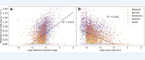
Individual regression models indicate that wetland fraction, area, perimeter, and temperature are the strongest individual quantitative predictors of lake methane ebullition (Table 3). The categorical test variable region has the highest predictive power (adj. R² = 0.320) of all of the variables tested, indicating strong spatial autocorrelation in the data set. LWF has the second-highest individual predictive power (adj. R² = 0.211; Figure 3A), followed by lake area (adj. R² = 0.201; Figure 3B). Of the remaining environmental variables, perimeter has moderate predictive power (adj. R² = 0.176) but is highly correlated with area (adj. R² = 0.899) and thus was excluded from subsequent multiple regression models. Temperature, both annual (adj. R² = 0.147) and winter (adj. R² = 0.157), is a moderately important variable in the individual regression models. The BR (adj. R² = 0.166, Table S.3) does not correlate as strongly as LWF, demonstrating that LWF is a physically meaningful variable rather than simply a function of lake morphology.

Figure 3. Methane ebullitive flux versus (A) lake wetland fraction, and (B) lake area with corresponding individual regression models.

SOC, permafrost, lake depth, and greenness are weak predictors of lake methane ebullition. These remaining representative predictor variables all have individual adjusted R² < 0.15. In the case of SOC, other variables from the same data set have higher adjusted R² values (Table S.3), but SOC was chosen as the representative variable because organic carbon availability in the form of DOC or SOC is a commonly considered variable in other regression-based studies and is known to have a physical link to methane production (e.g., Wik et al. 2016). Depth and greenness were found to have low adjusted R² values (0.029 and 0.016), but they are only available in smaller sample sizes and are biased toward large lakes.

A multiple regression model combining LWF, area, and temperature performs best of the models considering three variables, with an adjusted R² of 0.325 (Table 4). This model performs better than the model regressed solely on region (adj. R² = 0.320), which has the highest individual predictive power and accounts for numerous geographically dependent variables. Adding region-specific coefficients to the leading multivariate model (the “:” operator in Table 4) further increases the predictive power (adj. R² = 0.481) without loss of information (AIC = 2,430). Furthermore, for the model using lake area, LWF, and SOC, all variables are significant (p < 0.005) except for SOC. Multiple regression models using permafrost and SOC have adjusted R² values less than that of region alone (adj. R² = 0.237 and 0.227; Table 3). The models including lake depth and greenness performed significantly worse than all other models (adj. R² = 0.086 and 0.037; Table 4).

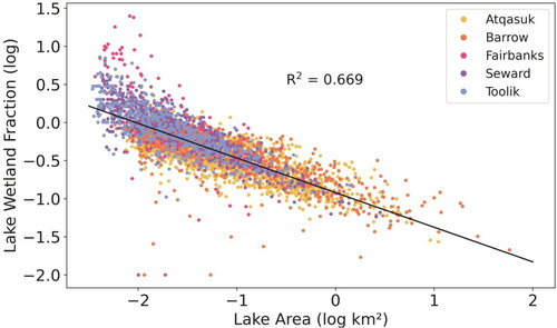
As anticipated (e.g., Murakami et al. 2019), some variables are spatially correlated with each other. Region is correlated with temperature (adj. R² = 0.989; Figure 4) providing an explanation for the predictive power of region. Similarly, LWF, the best individual predictor, is highly correlated with lake area, with an adjusted R² of 0.669. Perimeter is similarly correlated with LWF, with an adjusted R² of 0.516.

Figure 4. Observed linear relationship between lake area and lake wetland fraction.

Discussion

Our broad-scale results broadly agree with more detailed, regional regression-based studies (e.g., Bastviken et al. 2004; Praetzel, Schmiedeskamp, and Knorr 2021, Table S.1) reporting the importance of lake area, temperature, or both to lake methane ebullition emissions, although we find weaker correlations. Our finding that LWF is a leading predictor of ebullition (adj. R² = 0.221) supports previous findings that vegetated littoral zones generate higher ebullitive fluxes (Juutinen et al. 2003), likely due to the decomposition of buried organic matter (Wik et al. 2018). Additionally, we find that Fairbanks, which is the only region located in the discontinuous permafrost zone, has the highest mean ebullitive flux per lake (Table 1), which matches previous fine-scale studies (e.g., Walter Anthony et al. 2021). Although the reported correlations of these fine-scale studies are often stronger than the ones presented here, fine-scale studies also consider far fewer lakes and continuous spatial domains.

Despite general agreement with field-intensive studies, there are some discrepancies when it comes to depth and greenness. Many of these smaller scale studies find trophic status to be a strong predictor of ebullition (e.g., Sepulveda-Jauregui et al. 2015; DelSontro et al. 2016; Zhou et al. 2020). For example, Sepulveda-Jauregui et al. (2015) found that total nitrogen (R² = 0.32) is a leading predictor of methane ebullition for forty Alaskan lakes. We find that greenness, another proxy for trophic status, is a weak predictor at best (adj. R² = 0.016, n = 1,061), however. Similarly, although Bastviken et al. (2004) found that the probability of ebullition decreases from ∼80 percent at 0.5 to 1 m to ∼10 percent at 4 to 8 m depth, we find little relationship between depth and ebullition (adj. R² = 0.029, n = 1,224). Nevertheless, both variables are still considered significant with p < 0.001. These weak relationships are likely due to the spatial scales of the depth and greenness data sets, which only include lakes > 10 ha in area, with presumably low emissions per unit area. To replicate fine-scale relationships at the broad scales relevant to global methane, higher spatial resolution data are necessary for the lake depth and greenness variables.

Like previous broad-scale studies, our regression analyses using widely available geospatial data sets spanning thousands of lakes yield modest but statistically significant empirical correlations, thus offering a complementary way to evaluate the conclusions of smaller field studies. Our best model using lake area, temperature, and LWF (adj. R² = 0.325, n = 5,130) performs slightly better than leading multivariate models from similar studies such as Deemer and Holgerson (2021; (water-body type + latitude + chl a + area, adj. R² = 0.29, N = 103) and DelSontro, Beaulieu, and Downing (2019; area * total phosphorus, R² = 0.292, n = 101), even when considering significantly more lakes. We attribute these promising results to our selection of the top three predictors from numerous candidates. Still, finer scale studies, particularly for less than 100 lakes find stronger relationships (e.g., DelSontro et al. 2016; Praetzel, Schmiedeskamp, and Knorr 2021), likely because they include ebullition-relevant variables that can only be obtained from field work.

For purely mathematical reasons, larger studies are expected to yield lower coefficients of determination than studies with small sample sizes in simple linear regression (Ali 1987). We find that increased spatial scale provides a second reason for this observed decrease in predictive relationship with sample size, as strong regional trends become less evident when examining the data in aggregate. Similarly, Xu and Jin (2019) found a local, rather than global, model better fitted data in a study of online travel searches. This property is known as Simpson’s Paradox and is rarely discussed in geography (Sachdeva and Fotheringham 2023). Simpson’s Paradox is evident when examining depth, for example. When analyzing each region separately, we find adjusted R² = 0.120 (n = 125) in Seward, whereas adjusted R² = −0.049 in Fairbanks (n = 18), following region-specific trends. This observation, in combination with the lack of data for small lakes in the depth and greenness data sets, explains the absence of the strong depth and trophic-status relationships with ebullition described in the literature. Although depth and greenness were weak predictors on all lakes in aggregate, when regressed on a location-specific basis, they showed moderate trends with R² up to 0.120, better matching the regional studies. Because region, which appears to be a strong individual predictor, is specific to this study and thus not replicable, we only demonstrate the potential predictive power of the unmeasured variables for which region is a proxy in one multivariate regression model. As demonstrated, though, seeking regional trends might be more useful in future studies than a single global model. The main challenge is determining the appropriate size for each region, but there are statistical methods that could be implemented for this purpose (Root 2012).

Although lake area is a frequently cited predictor for methane ebullition in both field-based and broad-scale studies, our individual regression results indicate that LWF is equally important and might even be an underlying driver for the observed importance of area. The collinearity between lake area and LWF indicates that smaller lakes tend to be shallower and contain a greater proportion of land–water interface habitat, which often supports wetlands (Figure 4). This high correlation is in part due to the littoral class, which scales with lake perimeter, and is itself a correlate of lake area. Furthermore, our method for calculating wetland fraction is scale-sensitive and yields larger values for smaller lakes, although with better predictive power than the purely geometric BR. The classic Shoreline Development Index (SDI) has similar scale dependence (Seekell, Cael, and Byström 2022). Thus, small or sinuous lakes have higher wetland fractions, regardless of land-cover type. Although regression studies cannot determine causality between predictor variables, wetland presence is better supported as a mechanism for methane production than lake area per se (Juutinen et al. 2003; Kyzivat et al. 2022). Studies reporting high correlations between lake area and area-normalized methane flux (e.g., Stackpoole et al. 2017; Sanches et al. 2019; Engram et al. 2020) could therefore be more appropriately interpreted as describing high correlations with unmeasured shallow and vegetated water. This interpretation is consistent with littoral zone studies reporting higher per-unit flux from vegetated littoral zones than from open lake centers (Juutinen et al. 2003; Walter Anthony et al. 2016; Kyzivat et al. 2022).

Furthermore, as wetlands and LWF are difficult to classify in remotely sensed imagery, the strength of their correlation can vary based on method. In a similarly broad-scale analysis, Kyzivat et al. (2022) found that statistically significant regional correlations between lake emergent vegetation coverage and lake area never exceeded nonadjusted R² = 0.5, with a regionally aggregated R² = 0.124 (considerably lower than our own finding of nonadjusted R² = 0.669 for all sites combined; Figure 4). This discrepancy is very likely due to different methodologies and quantities being compared (i.e., lake emergent vegetation coverage vs. wetland fraction). Future work should consider more universally applicable methods for estimating LWF, such as that for littoral area (Seekell et al. 2021).

Limitations of this study include a heterogeneous spatial domain and uncertain, multicollinear study variables. SoilGrids-derived variables like SOC are highly interpolated and suffer from the modifiable area unit problem (Dark and Bram 2007), and so might not correctly characterize the soil margins surrounding or underlying individual lakes. HydroLakes depths are modeled estimates, and ABoVE land cover and wetland classes are nonexhaustive. SAR, which is currently underrepresented in the geographic literature, could be used to produce vegetation, lake area, and ebullition data sets, extending our findings to an even broader spatial domain when coupled with smaller, field-based studies. The forthcoming NASA-ISRO Synthetic Aperture Radar (NISAR; Kellogg et al. 2020) and recently launched Surface Water and Ocean Topography (SWOT; Fu et al. 2012) satellite radar missions, for example, might improve Arctic-boreal wetland mapping capability over Landsat-based approaches. These upcoming satellite missions have strong potential to improve climate-impact monitoring in the Arctic over broad spatial domains beyond mapping wetlands due to their ability to collect repeated observations in low light and cloudy conditions. From a statistical standpoint, the inherent correlations between certain variables, such as temperature and region or lake area and LWF, challenge the reliability of multiple linear regression models built from them. The latter collinearity, however, suggests that LWF (which tends to increase in smaller, shallower lakes) is a likely physical driver of the widely reported correlation between methane flux and lake area (e.g., Stackpoole et al. 2017; Sanches et al. 2019).

Regardless of these limitations, this study offers a straightforward demonstration of the value of using large environmental data sets to improve understanding of methane emissions, particularly from ebullition, over landscape-relevant scales. Lake ebullition is difficult to ascertain due to its spatial and temporal heterogeneity; thus, using large data sets to estimate ebullitive methane fluxes from lakes, as this study demonstrates, would be highly beneficial for estimating methane ebullition in regions across the pan-Arctic. We conclude that LWF is an underappreciated yet important predictor of lake methane ebullition, and that broad-scale geospatial studies of known lake attributes can complement conclusions drawn from smaller, field-intensive studies. Furthermore, to the best of our knowledge, our leading model (area + temperature + LWF, adj. R² = 0.325, n = 5,130) performs better than leading models from other broad-scale, regression-based ebullition studies. Future work should continue to accumulate field and remotely sensed data sets of other lake attributes such as DOC, colored dissolved organic matter, watershed attributes, topography, and vegetation phenology (Johnston et al. 2020), as the modest predictive power of current regression models suggests that spatial variations in ebullitive methane flux (and likely diffusive, plant-mediated flux, and storage fluxes as well) are not fully captured using existing geospatial data sets. Identifying the unmeasured spatially autocorrelated variables for which region is a proxy could also help to improve the predictive power of future models. Furthermore, higher resolution estimates for lake depth and greenness could help to improve estimates of ebullition over broad spatial domains if they are not biased toward large lakes. Future ebullition studies should also consider incorporating LWF in their analyses, as inclusion of this variable should improve landscape-scale assessments of Arctic-boreal lake methane emissions to the atmosphere.

Disclosure Statement

No potential conflict of interest was reported by the authors.

Supplemental Material

Supplemental data for this article can be accessed on the publisher’s site at https://doi.org/10.1080/24694452.2023.2216296. Experimental details and code in this study can be accessed at STTM-supporting_material-final.pdf.

Additional information

Funding

This work was funded by the following NASA programs: Future Investigators in NASA Earth and Space Science and Technology (FINESST) Grant Number 80NSSC19K1361, managed by Dr. Kathy Hibbard; Terrestrial Ecology Program Arctic-Boreal Vulnerability Experiment (ABoVE) Grant Numbers 80NSSC19M0104 and 80NSSC22K1237, managed by Dr. Hank Margolis and Dr. Michael Falkowski.

Notes on contributors

Michela J. Savignano

MICHELA J. SAVIGNANO is a Graduate Student in the Department of Geography and the Cooperative Institute for Research in Environmental Sciences at the University of Colorado, Boulder, CO 80309. E-mail: [email protected]. Her research interests include remote sensing of the cryosphere and ice sheet hydrology.

Ethan D. Kyzivat

ETHAN D. KYZIVAT is a Daly Postdoctoral Fellow in the Department of Earth and Planetary Sciences, Harvard University, Cambridge, MA 02138. E-mail: [email protected]. His research interests include the carbon cycle through high-resolution remote sensing of lakes and wetlands, with a focus on the Arctic.

Laurence C. Smith

LAURENCE C. SMITH is the John Atwater and Diana Nelson University Professor of Environmental Studies in the Institute at Brown for Environment & Society and the Department of Earth, Environmental and Planetary Sciences at Brown University, Providence, RI 02912. E-mail: [email protected]. His research interests include the Arctic, water resources, and satellite remote sensing technologies.

Melanie Engram

MELANIE ENGRAM is a Researcher at the Water and Environmental Research Center at the University of Alaska, Fairbanks, AK 99775. E-mail: [email protected]. Her research interests include the use of space-borne synthetic aperture radar (SAR) in a geospatial environment (GIS) to study lakes, methane emissions from lakes, and thermokarst activity in the Arctic and sub-Arctic.

References

- Aben, R. C., N. Barros, E. Van Donk, T. Frenken, S. Hilt, G. Kazanjian, L. P. Lamers, E. T. Peeters, J. G. Roelofs, L. N. de Senerpont Domis, et al. 2017. Cross continental increase in methane ebullition under climate change. Nature Communications 8 (1):1682. doi: 10.1038/s41467-017-01535-y.
- Ali, M. A. 1987. Effect of sample size on the size of the coefficient of determination in simple linear regression. Journal of Information and Optimization Sciences 8 (2):209–19. doi: 10.1080/02522667.1987.10698887.
- Arctic Monitoring and Assessment Programme. 2015. AMAP assessment 2015: Methane as an Arctic climate forcer. Oslo, Norway: Arctic Monitoring and Assessment Programme.
- Bastviken, D., J. Cole, M. Pace, and L. Tranvik. 2004. Methane emissions from lakes: Dependence of lake characteristics, two regional assessments, and a global estimate. Global Biogeochemical Cycles 18 (4): 238. doi: 10.1029/2004GB002238.
- Bastviken, D., L. J. Tranvik, J. A. Downing, P. M. Crill, and A. Enrich-Prast. 2011. Freshwater methane emissions offset the continental carbon sink. Science 331 (6013):50. doi: 10.1126/science.1196808.
- Cooley, S. W., L. C. Smith, J. C. Ryan, L. H. Pitcher, and T. M. Pavelsky. 2019. Arctic‐boreal lake dynamics revealed using CubeSat imagery. Geophysical Research Letters 46 (4):2111–20. doi: 10.1029/2018GL081584.
- Dark, S. J., and D. Bram. 2007. The modifiable areal unit problem (MAUP) in physical geography. Progress in Physical Geography: Earth and Environment 31 (5):471–79. doi: 10.1177/0309133307083294.
- Deemer, B. R., and M. A. Holgerson. 2021. Drivers of methane flux differ between lakes and reservoirs, complicating global upscaling efforts. Journal of Geophysical Research: Biogeosciences 126 (4):e2019JG005600. doi: 10.1029/2019JG005600.
- DelSontro, T., J. J. Beaulieu, and J. A. Downing. 2019. Greenhouse gas emissions from lakes and impoundments: Upscaling in the face of global change. Limnology and Oceanography Letters 3 (3):64–75. doi: 10.1002/lol2.10073.
- DelSontro, T., L. Boutet, A. St‐Pierre, P. A. del Giorgio, and Y. T. Prairie. 2016. Methane ebullition and diffusion from northern ponds and lakes regulated by the interaction between temperature and system productivity. Limnology and Oceanography 61 (Suppl. 1):S62–S77. doi: 10.1002/lno.10335.
- Dhakal, S., J. C. Minx, F. L. Toth, A. Abdel-Aziz, M. J. Figueroa Meza, K. Hubacek, I. G. C. Jonckheere, Y. G. Kim, G. F. Nemet, S. Pachauri, et al. 2022. Climate change 2022: Mitigation of climate change. Contribution of Working Group III to the Sixth Assessment Report of the Intergovernmental Panel on Climate Change, ed. P. R. Shukla, J. Skea, R. Slade, A. Al Khourdajie, R. van Diemen, D. McCollum, M. Pathak, S. Some, P. Vyas, R. Fradera, M. Belkacemi, A. Hasija, G. Lisboa, S. Luz, and J. Malley. Cambridge, UK: Cambridge University Press. doi: 10.1017/9781009157926.004.
- Engram, M., K. W. Anthony, F. J. Meyer, and G. Grosse. 2013. Synthetic aperture radar (SAR) backscatter response from methane ebullition bubbles trapped by thermokarst lake ice. Canadian Journal of Remote Sensing 38 (6):667–82. doi: 10.5589/m12-054.
- Engram, M. J., K. Walter Anthony, and F. J. Meyer. 2020. ABoVE: SAR-based methane ebullition flux from lakes, five regions, Alaska, 2007–2010. ORNL DAAC, Oak Ridge, TN. doi: 10.3334/ORNLDAAC/1790.
- Engram, M., K. M. Walter Anthony, T. Sachs, K. Kohnert, A. Serafimovich, G. Grosse, and F. J. Meyer. 2020. Remote sensing northern lake methane ebullition. Nature Climate Change 10 (6):511–17. doi: 10.1038/s41558-020-0762-8.
- Fu, L. L., D. Alsdorf, R. Morrow, E. Rodriguez, and N. Mognard. 2012. SWOT: The surface water and ocean topography mission: Wide-swath altimetric elevation on Earth. Pasadena, CA: Jet Propulsion Laboratory, National Aeronautics and Space Administration.
- Haslwanter, T. 2016. An introduction to statistics with Python with applications in the life sciences. Cham, Switzerland: Springer International.
- Johnson, M. S., E. Matthews, J. Du, V. Genovese, and D. Bastviken. 2022. Methane emission from global lakes: New spatiotemporal data and observation‐driven modeling of methane dynamics indicates lower emissions. Journal of Geophysical Research: Biogeosciences 127 (7):e2022JG006793. doi: 10.1029/2022JG006793.
- Johnston, S. E., R. G. Striegl, M. J. Bogard, M. M. Dornblaser, D. E. Butman, A. M. Kellerman, K. P. Wickland, D. C. Podgorski, and R. G. Spencer. 2020. Hydrologic connectivity determines dissolved organic matter biogeochemistry in northern high‐latitude lakes. Limnology and Oceanography 65 (8):1764–80. doi: 10.1002/lno.11417.
- Julian, J. P., R. J. Davies-Colley, C. L. Gallegos, and T. V. Tran. 2013. Optical water quality of inland waters: A landscape perspective. Annals of the Association of American Geographers 103 (2):309–18. doi: 10.1080/00045608.2013.754658.
- Juutinen, S., J. Alm, T. Larmola, J. T. Huttunen, M. Morero, P. J. Martikainen, and J. Silvola. 2003. Major implication of the littoral zone for methane release from boreal lakes. Global Biogeochemical Cycles 17 (4):105. doi: 10.1029/2003GB002105.
- Kellogg, K., P. Hoffman, S. Standley, S. Shaffer, P. Rosen, W. Edelstein, C. Dunn, C. Baker, P. Barela, Y. Shen, et al. 2020. NASA-ISRO synthetic aperture radar (NISAR) mission. In 2020 IEEE Aerospace Conference, 1–21). Big Sky, MT: IEEE. doi: 10.1109/AERO47225.2020.9172638.
- Kohnert, K., B. Juhls, S. Muster, S. Antonova, A. Serafimovich, S. Metzger, J. Hartmann, and T. Sachs. 2018. Toward understanding the contribution of waterbodies to the methane emissions of a permafrost landscape on a regional scale—A case study from the Mackenzie delta, Canada. Global Change Biology 24 (9):3976–89. doi: 10.1111/gcb.14289.
- Kuhn, C., and D. Butman. 2021. ABoVE: Lake growing season green surface reflectance trends, AK and Canada, 1984–2019. Oak Ridge, TN: ORNL DAAC. doi: 10.3334/ORNLDAAC/1866.
- Kuhn, M. A., R. K. Varner, D. Bastviken, P. Crill, S. MacIntyre, M. Turetsky, K. Walter Anthony, A. D. McGuire, and D. Olefeldt. 2021. BAWLD-CH 4: A comprehensive dataset of methane fluxes from boreal and Arctic ecosystems. Earth System Science Data 13 (11):5151–89. doi: 10.5194/essd-13-5151-2021.
- Kyzivat, E. D., L. C. Smith, F. Garcia‐Tigreros, C. Huang, C. Wang, T. Langhorst, J. V. Fayne, M. E. Harlan, Y. Ishitsuka, D. Feng, et al. 2022. The importance of lake emergent aquatic vegetation for estimating arctic‐boreal methane emissions. Journal of Geophysical Research: Biogeosciences 127 (6):e2021JG006635. doi: 10.1029/2021JG006635.
- Kyzivat, E. D., L. C. Smith, L. H. Pitcher, J. V. Fayne, S. W. Cooley, M. G. Cooper, S. N. Topp, T. Langhorst, M. E. Harlan, C. Horvat, et al. 2019. A high-resolution airborne color-infrared camera water mask for the NASA ABoVE campaign. Remote Sensing 11 (18):2163. doi: 10.3390/rs11182163.
- Lu, X., D. J. Jacob, Y. Zhang, J. D. Maasakkers, M. P. Sulprizio, L. Shen, Z. Qu, T. R. Scarpelli, H. Nesser, R. M. Yantosca, et al. 2021. Global methane budget and trend, 2010–2017: Complementarity of inverse analyses using in situ (GLOBALVIEWplus CH 4 ObsPack) and satellite (GOSAT) observations. Atmospheric Chemistry and Physics 21 (6):4637–57. doi: 10.5194/acp-21-4637-2021.
- Ludwig, S. M., S. M. Natali, P. J. Mann, J. D. Schade, R. M. Holmes, M. Powell, G. Fiske, and R. Commane. 2022. Using machine learning to predict inland aquatic CO2 and CH4 concentrations and the effects of wildfires in the Yukon-Kuskokwim Delta, Alaska. Global Biogeochemical Cycles 36 (4):e2021GB007146. doi: 10.1029/2021GB007146.
- Matthews, E., M. S. Johnson, V. Genovese, J. Du, and D. Bastviken. 2020. Methane emission from high latitude lakes: Methane-centric lake classification and satellite-driven annual cycle of emissions. Scientific Reports 10 (1):12465. doi: 10.1038/s41598-020-68246-1.
- McGuire, A. D., L. G. Anderson, T. R. Christensen, S. Dallimore, L. Guo, D. J. Hayes, M. Heimann, T. D. Lorenson, R. W. Macdonald, and N. Roulet. 2009. Sensitivity of the carbon cycle in the Arctic to climate change. Ecological Monographs 79 (4):523–55. doi: 10.1890/08-2025.1.
- Messager, M. L., B. Lehner, G. Grill, I. Nedeva, and O. Schmitt. 2016. Estimating the volume and age of water stored in global lakes using a geo-statistical approach. Nature Communications 7 (1):13603. doi: 10.1038/ncomms13603.
- Murakami, D., B. Lu, P. Harris, C. Brunsdon, M. Charlton, T. Nakaya, and D. A. Griffith. 2019. The importance of scale in spatially varying coefficient modeling. Annals of the American Association of Geographers 109 (1):50–70. doi: 10.1080/24694452.2018.1462691.
- Muster, S., K. Roth, M. Langer, S. Lange, F. Cresto Aleina, A. Bartsch, A. Morgenstern, G. Grosse, B. Jones, A. B. K. Sannel, et al. 2017. PeRL: A circum-Arctic permafrost region pond and lake database. Earth System Science Data 9 (1):317–48. doi: 10.5194/essd-9-317-2017.
- Negandhi, K., I. Laurion, M. J. Whiticar, P. E. Galand, X. Xu, and C. Lovejoy. 2013. Small thaw ponds: An unaccounted source of methane in the Canadian High Arctic. PLoS ONE 8 (11):e78204. doi: 10.1371/journal.pone.0078204.
- Olefeldt, D., M. Hovemyr, M. A. Kuhn, D. Bastviken, T. J. Bohn, J. Connolly, P. Crill, E. S. Euskirchen, S. A. Finkelstein, H. Genet, et al. 2021. The Boreal–Arctic Wetland and Lake Dataset (BAWLD). Earth System Science Data 13 (11):5127–49. doi: 10.5194/essd-13-5127-2021.
- Pastick, N. J., M. T. Jorgenson, B. K. Wylie, S. J. Nield, K. D. Johnson, and A. O. Finley. 2015. Distribution of near-surface permafrost in Alaska: Estimates of present and future conditions. Remote Sensing of Environment 168:301–15. doi: 10.1016/j.rse.2015.07.019.
- Poggio, L., L. M. De Sousa, N. H. Batjes, G. Heuvelink, B. Kempen, E. Ribeiro, and D. Rossiter. 2021. SoilGrids 2.0: Producing soil information for the globe with quantified spatial uncertainty. SOIL 7 (1):217–40. doi: 10.5194/soil-7-217-2021.
- Praetzel, L. S. E., M. Schmiedeskamp, and K. H. Knorr. 2021. Temperature and sediment properties drive spatiotemporal variability of methane ebullition in a small and shallow temperate lake. Limnology and Oceanography 66 (7):2598–2610. doi: 10.1002/lno.11775.
- Rantanen, M., A. Y. Karpechko, A. Lipponen, K. Nordling, O. Hyvärinen, K. Ruosteenoja, T. Vihma, and A. Laaksonen. 2022. The Arctic has warmed nearly four times faster than the globe since 1979. Communications Earth & Environment 3 (1):168. doi: 10.1038/s43247-022-00498-3.
- Root, E. D. 2012. Moving neighborhoods and health research forward: Using geographic methods to examine the role of spatial scale in neighborhood effects on health. Annals of the Association of American Geographers 102 (5):986–95. doi: 10.1080/00045608.2012.659621.
- Sachdeva, M., and A. S. Fotheringham. 2023. A geographical perspective on Simpson’s Paradox. Journal of Spatial Information Science 26 (26):1–25. doi: 10.5311/JOSIS.2023.26.212.
- Sanches, L. F., B. Guenet, C. C. Marinho, N. Barros, and F. de Assis Esteves. 2019. Global regulation of methane emission from natural lakes. Scientific Reports 9 (1):255. doi: 10.1038/s41598-018-36519-5.
- Saunois, M., A. R. Stavert, B. Poulter, P. Bousquet, J. G. Canadell, R. B. Jackson, P. A. Raymond, E. J. Dlugokencky, S. Houweling, P. K. Patra, et al. 2020. The global methane budget 2000–2017. Earth System Science Data 12 (3):1561–1623. doi: 10.5194/essd-12-1561-2020.
- Seekell, D., B. B. Cael, and P. Byström. 2022. Problems with the Shoreline Development Index—A widely used metric of lake shape. Geophysical Research Letters 49 (10):e98499. doi: 10.1029/2022GL098499.
- Seekell, D., B. Cael, S. Norman, and P. Byström. 2021. Patterns and variation of littoral habitat size among lakes. Geophysical Research Letters 48 (20):e2021GL095046. doi: 10.1029/2021GL095046.
- Sepulveda-Jauregui, A., K. M. Walter Anthony, K. Martinez-Cruz, S. Greene, and F. Thalasso. 2015. Methane and carbon dioxide emissions from 40 lakes along a north–south latitudinal transect in Alaska. Biogeosciences 12 (11):3197–3223. doi: 10.5194/bg-12-3197-2015.
- Smith, L. C. 2002. Emerging applications of Interferometric Synthetic Aperture Radar (InSAR) in geomorphology and hydrology. Annals of the Association of American Geographers 92 (3):385–98. doi: 10.1111/1467-8306.00295.
- Smith, L. C., Y. Sheng, G. M. MacDonald, and L. D. Hinzman. 2005. Disappearing arctic lakes. Science 308 (5727):1429. doi: 10.1126/science.1108142.
- Stackpoole, S. M., D. E. Butman, D. W. Clow, K. L. Verdin, B. V. Gaglioti, H. Genet, and R. G. Striegl. 2017. Inland waters and their role in the carbon cycle of Alaska. Ecological Applications 27 (5):1403–20. doi: 10.1002/eap.1552.
- Thornton, M. M., R. Shrestha, Y. Wei, P. E. Thornton, S. Kao, and B. E. Wilson. 2020. Daymet: Daily surface weather data on a 1-km grid for North America, version 4. ORNL DAAC, Oak Ridge, TN. doi: 10.3334/ORNLDAAC/1840.
- Walter, K. M., L. C. Smith, and S. F. Chapin. 2007. Methane bubbling from northern lakes: Present and future contributions to the global methane budget. Philosophical Transactions Series A: Mathematical, Physical, and Engineering Sciences 365 (1856):1657–76. doi: 10.1098/rsta.2007.2036.
- Walter Anthony, K., R. Daanen, P. Anthony, T. Schneider von Deimling, C. L. Ping, J. P. Chanton, and G. Grosse. 2016. Methane emissions proportional to permafrost carbon thawed in Arctic lakes since the 1950s. Nature Geoscience 9 (9):679–82. doi: 10.1038/ngeo2795.
- Walter Anthony, K. M., P. Lindgren, P. Hanke, M. Engram, P. Anthony, R. P. Daanen, A. Bondurant, A. K. Liljedahl, J. Lenz, G. Grosse, et al. 2021. Decadal-scale hotspot methane ebullition within lakes following abrupt permafrost thaw. Environmental Research Letters 16 (3):035010. doi: 10.1088/1748-9326/abc848.
- Wang, G., X. Xia, S. Liu, L. Zhang, S. Zhang, J. Wang, N. Xi, and Q. Zhang. 2021. Intense methane ebullition from urban inland waters and its significant contribution to greenhouse gas emissions. Water Research 189:116654. doi: 10.1016/j.watres.2020.116654.
- Wang, J. A., D. Sulla-Menashe, C. E. Woodcock, O. Sonnentag, R. F. Keeling, and M. A. Friedl. 2019. ABoVE: Landsat-derived annual dominant land cover across ABoVE core domain, 1984–2014. Oak Ridge, TN: ORNL DAAC. doi: 10.3334/ORNLDAAC/1691.
- Wik, M., J. E. Johnson, P. M. Crill, J. P. DeStasio, L. Erickson, M. J. Halloran, M. F. Fahnestock, M. K. Crawford, S. C. Phillips, and R. K. Varner. 2018. Sediment characteristics and methane ebullition in three subarctic lakes. Journal of Geophysical Research: Biogeosciences 123 (8):2399–2411. doi: 10.1029/2017JG004298.
- Wik, M., R. K. Varner, K. W. Anthony, S. MacIntyre, and D. Bastviken. 2016. Climate-sensitive northern lakes and ponds are critical components of methane release. Nature Geoscience 9 (2):99–105. doi: 10.1038/ngeo2578.
- Xu, J., and C. Jin. 2019. Exploring spatiotemporal heterogeneity in online travel searches: A local spatial model approach. Geografisk Tidsskrift-Danish Journal of Geography 119 (2):146–62. doi: 10.1080/00167223.2019.1601575.
- Yvon-Durocher, G., A. P. Allen, D. Bastviken, R. Conrad, C. Gudasz, A. St-Pierre, N. Thanh-Duc, and P. A. Del Giorgio. 2014. Methane fluxes show consistent temperature dependence across microbial to ecosystem scales. Nature 507 (7493):488–91. doi: 10.1038/nature13164.
- Zhou, Y., K. Song, R. Han, S. Riya, X. Xu, S. Yeerken, S. Geng, Y. Ma, and A. Terada. 2020. Nonlinear response of methane release to increased trophic state levels coupled with microbial processes in shallow lakes. Environmental Pollution 265 (Pt. B):114919. doi: 10.1016/j.envpol.2020.114919.