The importance of riparian plant orientation in river flow: implications for flow structures and drag

Abstract

In a series of high resolution numerical modelling experiments, we incorporated submerged riparian plants into a computational fluid dynamics (CFD) model used to predict flow structures and drag in river flow. Individual plant point clouds were captured using terrestrial laser scanning (TLS) and geometric characteristics quantified. In the first experiment, flow is modelled around three different plant specimens of the same species (Prunus laurocerasus). In the second experiment, the orientation of another specimen is incrementally rotated to modify the flow-facing structure when foliated and defoliated. Each plant introduces a unique disturbance pattern to the normalized downstream velocity field, resulting in spatially heterogeneous and irregularly shaped velocity profiles. The results question the extent to which generalized velocity profiles can be quantified for morphologically complex plants. Incremental changes in plant orientation introduce gradual changes to the downstream velocity field and cause a substantial range in the quantified drag response. Form drag forces are up to an order of magnitude greater for foliated plants compared to defoliated plants, although the mean drag coefficient for defoliated plants is higher (1.52 defoliated; 1.03 foliated). Variation in the drag coefficients is greatest when the plant is defoliated (up to ∼210% variation when defoliated, ∼80% when foliated).

Keywords:

• Riparian vegetation
• plant orientation
• CFD
• drag coefficient
• flow-facing structure

Introduction

Vegetation is abundant in lowland rivers and has a significant influence on their hydraulic, geomorphological, and ecological functioning. Riparian vegetation can significantly increase local and boundary flow resistance and thus cause a reduction in flow velocity (Kouwen et al. 1969). This strongly reduces conveyance (Kadlec 1990; Nepf et al. 2007) and creates regions of reduced shear stress that promote local sedimentation (Sand-Jensen 1998), influencing flow and sediment transport pathways (McBride et al. 2007), biota (Petr 2000), and determining the local flow conditions (Folkard 2016). Vegetation is therefore critically important in controlling the hydrodynamics of aquatic ecosystems (Nikora 2010).

The process by which vegetation extracts energy from open channel flow is through drag. The total drag force acting on vegetation is the sum of skin friction (viscous) drag exerted over the vegetation surface, and form (pressure) drag resulting from flow separation (Bakry et al. 1992; Siniscalchi and Nikora 2012). For riparian plant species, form drag dominates over skin friction drag (Nikora 2010; Västilä and Järvelä 2014) and can account for 90–97% of the total drag in turbulent flows (Lilly 1967; Vogel 1994; Stoesser et al. 2010). Although the drag response is well understood for simple geometric shapes (e.g. for cylinders a drag coefficient value of unity is accepted for Re in the range 10³ to 3 × 10⁵; Panton 1984; Tritton 1988), it is less well understood for the complex geometries of natural vegetation (Marjoribanks et al. 2014a). At the individual plant-scale, the drag response is further complicated by the multitude of stem- and leaf-scales (de Langre 2008; Albayrak et al. 2012; Luhar and Nepf 2011), variation in plant morphology (Wilson et al. 2003), and reconfiguration of the dynamic plant morphology under hydrodynamic loading (Vogel 1994).

The plant morphology is defined as the physical plant structure, including the number of stems, the size and shape of the leaf body, and the vertical and horizontal distribution of vegetal elements (Manners et al. 2015). Plant morphology varies over time and space (Thomas et al. 2014) and differs depending on plant species, size, and patch densities (Naiman and Décamps 1997). Plant morphology influences flow field dynamics; for example, Manners et al. (2015) showed through the analysis of the downstream velocity field and sediment transport paths around individual plants for contrasting riparian vegetation species (Tamarix chinensis/Tamarix ramossissima and Populus fremontii) that the more complex, shrubby morphology of Tamarix alters the flow fields more than the single stemmed, relatively simpler morphology of the Populus. Plant morphology therefore influences flow through, over and around vegetation (Tempest et al. 2015), affecting the turbulent flow regimes across a range of spatial scales (Nikora et al. 2012). Different plant species, with distinct morphologies, can therefore cause different effects on the flow and drag response (Watts and Watts 1990).

Differences in the plant morphology are not limited to different species, as plants of the same species can show morphological variety and a range of sizes (Siniscalchi and Nikora 2012). In laboratory flume experiments, it remains uncertain whether the use of “representative” plant morphologies is sufficient to understand the flow around specific species when using plant surrogates (Thomas et al. 2014). Although variation in the biomechanical and morphological factors within and between plant species have previously been described (Oplatka 1998; Stone et al. 2013; Whittaker et al. 2013), the effect on flow field dynamics are yet to be fully quantified. It is therefore suggested that for an individual species, plants with different morphologies could introduce substantial differences into the flow field.

Computational fluid dynamics (CFD) modelling offers a methodology to simulate flow that is of practical importance, but notoriously difficult to measure (Hardy et al. 2003). Discretization methods now allow vegetation to be treated as a porous blockage (Marjoribanks et al. 2014a), moving beyond the highly idealized and simplified plant representations that are used even in some recent numerical modelling studies (e.g. Liu et al. 2018). This method allows accurate and realistic three-dimensional plant morphologies to be incorporated into the numerical domain and has recently been extended so the volumetric canopy morphology of plants can be measured and explicitly represented in a CFD model (Boothroyd et al. 2016a, 2017). This provides a new approach to study flow-vegetation interactions.

Here, we provide an improved process–understanding of how the presentation of a plant to flow influences the flow field dynamics. We define plant presentation as the amount of volumetric canopy “seen” by the incident flow, relating to the flow-facing structure that is orientation dependent. This is achieved by accurately capturing the distribution of vegetal elements over the three-dimensional plant structure using terrestrial laser scanning (TLS), and incorporating these realistic plant representations into a CFD model. Using this approach, we have designed a series of numerical modelling experiments (subdivided into experiments 1 and 2) that allow the influence of the presentation and orientation of the plant to the incident flow to be tested, to provide new insights into flow-vegetation interactions at the plant-scale.

1. Experiment 1 investigates flow and drag around three different plants of the same species (labelled Pl₁–Pl₃). The three specimens were selected for their approximate similarity in size and foliage density, but natural variation in plant morphology. The experiment is designed to highlight differences and similarities in flow field dynamics between plants of the same species.

2. Experiment 2 focuses on the orientation of a single plant in foliated and defoliated states. A fourth plant, of the same species used in experiment 1 (labelled Pl₄), is exposed to the incident flow and then the plant orientation is incrementally varied. This is initially done for the foliated state then repeated for the mechanically defoliated state. The experiment is designed to test the downstream velocity and drag sensitivity of the flow-facing structure, with the orientation of the plant incrementally changed between model runs.

In this article, high resolution numerical model predictions of the downstream velocity and pressure field around riparian plants are shown. We investigate flow structures and the drag response around different plants of the same species and incrementally modify plant orientations to assess the influence of changes in the flow-facing structure on flow field dynamics. Practical implications are discussed and then used to provide recommendations of best practice in future laboratory flume and numerical modelling experiments.

Methods

Plant characteristics

Prunus laurocerasus was selected as the plant species for use in this study. The species has an open framework with a complex branch and leaf structure, sharing morphological similarities to woody riverine vegetation species such as Populus nigra typically found on gravel bars (O’Hare et al. 2016). In experiment 1, the three specimens (labelled Pl₁, Pl₂, and Pl₃) have plant heights of ∼0.80 m. To assess changes in plant orientation and differences in the foliation state, a different specimen (Pl₄) was used in experiment 2. The specimen had a greater plant height to crown width ratio, with dimensions of 0.93 × 0.37 m when foliated and 0.91 × 0.17 m when mechanically defoliated (as described by Boothroyd et al. 2016a). Plant geometry characteristics are summarized in Table 1.

Table 1. Plant geometric characteristics and plant drag response (total domain drag, form drag, skin friction drag for the whole domain and drag coefficient) for experiment 1 (Pl₁, Pl₂, and Pl₃) and experiment 2 (Pl₄, defoliated_(Def) and foliated_(Fol) at 0° plant orientation).

Plant	Plant frontal area (m^2)	Plant volume (m^3)	Total domain drag force (N m^2)	Form drag force (N m^2)	Skin friction drag force for the whole domain (N m^2)	Ratio of form drag to skin friction drag for the whole domain (-)	Drag coefficient (-)
Pl1	0.282	0.0091	9.742	4.432	5.310	0.835	1.786
Pl2	0.260	0.0067	7.033	3.819	3.214	1.188	1.805
Pl3	0.342	0.0084	9.840	5.056	4.784	1.057	1.384
Pl4 Def	0.055	0.0012	4.431	0.148	4.283	0.035	1.540
Pl4 Fol	0.212	0.0050	5.746	1.742	4.004	0.435	1.243

TLS to capture plant morphology

Three-dimensional plant representations were acquired from a series of point clouds using TLS, the ground-based implementation of Light Detection And Ranging (LiDAR). LiDAR is the preferred tool for capturing remotely sensed three-dimensional measurements of vegetation (Vierling et al. 2008), with TLS used to accurately quantify plant structure and form (Moorthy et al. 2011) and improve estimates of above ground biomass (Disney et al. 2018). In this study, specimens were scanned in a controlled laboratory environment rather than in situ. Plants were scanned from multiple perspectives, and positioned 5 m from a RIEGL VZ-1000 scanner, as previously reported by Boothroyd et al. (2016a, 2017). Scans were collected from four opposing perspectives to minimize occlusion effects (Moorthy et al. 2008), with the mean distance between neighbouring points in the registered point clouds ∼0.0025 m. Riegl (2015) reported that at a distance of 10 m, the scanner has a range accuracy of 0.008 m and a precision of 0.005 m. The registered point clouds were then postprocessed, with the neighbourhood-based approach by Rusu et al. (2008) used to classify outliers and remove erroneous returns from the point clouds (Boothroyd et al. 2016a). This step is necessary to remove isolated points from the point cloud, specifically those off-centre hits caused by the position and size of the laser pulse footprint relative to the feature being scanned (Béland et al. 2014), which would otherwise lead to plant morphological errors and volumetric overestimation (Bienert et al. 2014).

Voxelization procedure

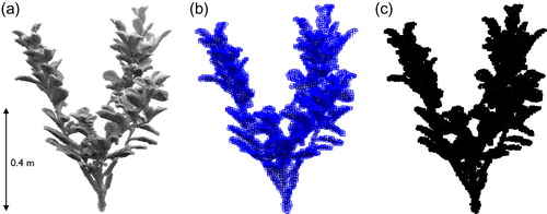
To reduce the number of postprocessed points but retain plant morphology, a voxelization procedure is applied. This followed the workflow developed by Jalonen et al. (2015) and Boothroyd et al. (2016a) to produce the voxelized plant representations (example shown for Pl₃ in Figure 1). During the voxelization procedure, initial point clouds with a ∼0.0025 m point spacing were converted to voxel arrays with a 0.01 m voxel size. Justification for the 0.01 m voxel size is partly provided by previous sensitivity analysis that showed similarity in the flow fields around plant sections represented by 0.005 m and 0.01 m voxel sizes (Boothroyd et al. 2016b), and the recommendation by Hosoi et al. (2013) that the voxel size should approximately correspond with the diameter of the smallest plant branches (∼0.01 m). However, the recommendation does not account for foliation. If the thinness of leaves (typically sub-mm) are taken into account, the volume of a single leaf is likely to be greatly overestimated by the 0.01 m voxel size. Therefore, foliated plant geometric characteristics will be overestimated (Hess et al. 2015) and this represents a limitation of our approach. Application of a finer voxel size could improve the representation of foliation; however, this would be limited by the instrument precision. A balance therefore exists between the instrument precision and plant characteristics, with the 0.01 m voxel size providing the best solution. The voxelization procedure considerably simplifies the point cloud, reducing the number of points from ∼300,000 to ∼8,500 voxels in Pl₃, and providing a binary occupied/unoccupied grid of voxels that are incorporated directly into the CFD model. For experiment 2, the voxelized plant representations are rotated about the vertical axis in 15° increments, thereby changing the plant orientation to the incident flow by 0° to 360° and providing 24 discrete orientations for each of the defoliated and foliated plants. The naming of plant orientations is arbitrary because it is dependent on the way the plant was oriented during the initial scanning process.

Figure 1. Stages of the voxelization process for the P. laurocerasus plant used in experiment 1 (Pl₃), showing: (a) the postprocessed point cloud containing ∼300,000 points, (b) the fitted octree structure with a cell size of 0.01 m, and (c) the voxelized plant representation at a 0.01 m voxel size (∼8,500 individual voxels).

CFD modelling

The numerical scheme involves a finite volume solution of the full three-dimensional Navier–Stokes equations in a Cartesian coordinate system, with the equations closed by applying a two-equation k-ε turbulence model modified using Renormalization Group Theory (RNG) (Yakhot and Orszag 1986). This model has been shown to outperform the standard k-ε turbulence model in regions of high strain, flow separation, and reattachment (Yakhot and Orszag 1986; Lien and Leschziner 1994; Hodskinson and Ferguson 1998; Bradbrook et al. 2000), is numerically stable (Hardy et al. 2005), and has been widely adopted in geomorphological CFD applications (Hodskinson and Ferguson 1998; Bradbrook et al. 2000; Marjoribanks et al. 2016). The convergence criterion was set such that the residuals of mass and momentum flux were reduced to 0.1% of the inlet flux, as has been applied in previous work (Ferguson et al. 2003; Lane et al. 2004; Marjoribanks et al. 2016). The CFD model has previously been validated against spatially distributed velocity measurements of flow around a submerged Hebe odora plant, with velocity measurements collected using an acoustic Doppler velocimeter (aDv) and showed very good general agreement for the three-dimensional mean flow (Boothroyd et al. 2017).

In experiment 1, a domain of 300 cells long, 100 cells wide, and 85 cells high was created at a spatial resolution of 0.01 m (2,550,000 grid cells). In experiment 2, a similar domain of 350 cells long, 120 cells wide, and 100 cells high was created at a spatial resolution of 0.01 m (4,200,000 grid cells). Domains of different sizes were required to accommodate the plant representations, whilst maximizing the computational efficiency.

The voxelized plant representations were incorporated into the CFD model using a mass flux scaling algorithm (MFSA) (Lane et al. 2002, 2004; Hardy et al. 2005), treating the plants as a numerical porosity (Marjoribanks et al. 2014b; Boothroyd et al. 2016a; Marjoribanks et al. 2016; Boothroyd et al. 2017). Because the spatial discretization of the domain is equal to the voxel size used to describe the plant, a binary blocked/unblocked numerical porosity treatment follows (Lane et al. 2004). This means that all permeability through the plant is explicitly represented by the grid-scale plant blockage.

The plant blockages were centred at the midline (0.5 Y/w) and positioned at 0.22 X/l in experiment 1, and 0.18 X/l in experiment 2. An overview of both numerical domains showing the position of the plants are shown in Figures 2(a) and 3(a). The flow-facing structure of the plants to the incident flow for experiments 1 and 2 are shown in Figures 2(b) and 3(b), respectively. Considerable differences in the flow-facing structure are shown between specimens of the same species (Figure 2(b), experiment 1). Similarly, Figure 3(b) (experiment 2) shows that the flow-facing structure of the defoliated and foliated plants is modified with changes in plant orientation from 0° to 180°. Based on the two-dimensional projection of each plant in the numerical domain, blockage ratios are reported in Figures 2(b) and 3(b). Between different specimens of the same species, and with changes in plant orientation, how the plant is “seen” by the incident flow is substantially altered. The differences in plant geometry characteristics between plants (Pl₁–Pl₄) are quantified in the results section.

Figure 2. (a) The domain used in the CFD model (experiment 1) to simulate flow around Pl₁–Pl₃. The blue values indicate the number of cells in each direction of the domain, the blue arrow demonstrates the flow direction, and the red dots show the position of extracted velocity profiles. (b) The presentation of the P. laurocerasus specimens, showing the flow-facing structure as viewed looking downstream from the domain inlet. The blockage ratio is shown in the bottom-left corner of each plot.

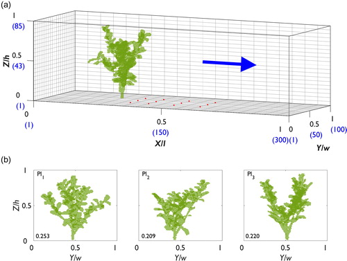
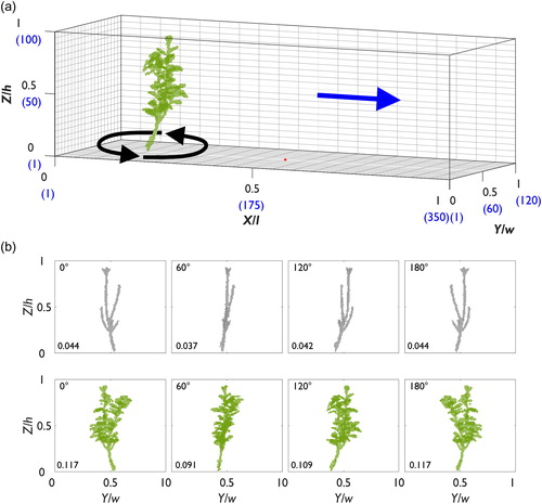
Figure 3. (a) The domain used in the CFD model (experiment 2) to simulate flow with incremental changes in plant orientation. The blue values indicate the number of cells in each direction of the domain, the blue arrow demonstrates the flow direction, and the red dot shows the position of the extracted velocity profiles. The black arrows indicate rotation around the base of the plant. (b) The presentation of the defoliated (top row) and foliated (bottom row) plant in the plant orientation range 0°–180°, showing the flow-facing structure as viewed looking downstream from the domain inlet. The blockage ratio is shown in the bottom-left corner of each plot.

Inlet conditions are kept the same throughout the numerical experiments, with downstream velocity set to 0.25 m/s (held constant over Z/h), and a turbulent intensity of 5% used. In each experiment, the flow was fully turbulent (Re 230,000 and 270,000) and subcritical (Fr 0.09 and 0.08). The outlet was defined using a fixed-pressure boundary condition where mass could enter and leave the domain. No modification has been applied to the turbulence model for either bed or domain sidewalls, which were treated as a non‐slip boundary, and the nonequilibrium wall function is applied which assumes local equilibrium of turbulence (y⁺ = 47) (Launder and Spalding 1974).

We present results with the downstream (u–) velocity field normalized on the inlet velocity. Velocity profiles were selected to cover the downstream range of wake separation and reattachment, with slices along the domain midline and outer plant edges used to further elucidate flow structures. In experiment 1, mean normalized downstream velocity profiles are calculated from Pl₁, Pl₂, and Pl₃. In experiment 2, mean normalized downstream velocity profiles are calculated for both foliation states from the 24 plant orientations. Furthermore, the pressure field (p) surrounding vegetation elements is resolved in the downstream direction and integrated over the lateral extent of the plant blockage to calculate the form drag response. This involves integrating the difference in pressure from immediately upstream and downstream of vegetal elements to calculate the net downstream force exerted on the plant. Calculation of form drag follows the standard method in aerodynamics for calculating drag from pressure (Anderson 1984), following the pressure coefficient approach: (1) $$F_{\mathrm{d}}={\int }_A\left(p_{\mathrm{f}}-p_{\mathrm{b}}\right)d{A}_{\mathrm{p}}$$(1) where F_d is the form drag force (N m²), p_f is the pressure at the blockage front (Pa), p_b is the pressure at the blockage back (Pa), d is the height of cells in the domain (m), and A_p is the reference area (m²). The reference area is taken as the plant frontal area, which is quantified from the voxelized plant representations. In addition to form drag, an estimate of the total domain drag is quantified by summing the difference in pressure from the inlet and outlet of the domain, and reapplying Equation (1)(1) $$F_{\mathrm{d}}={\int }_A\left(p_{\mathrm{f}}-p_{\mathrm{b}}\right)d{A}_{\mathrm{p}}$$(1) . With form drag subtracted from the total domain drag, the contribution of skin friction drag for the whole domain is estimated. The ratio of form to skin friction drag for the whole domain is then quantified.

Furthermore, form drag force is used to calculate the drag coefficient, following: (2) $$C_{\mathrm{d}}=\frac{F_{\mathrm{d}}}{\frac{1}{2}\rho u^2{A}_{\mathrm{p}}}$$(2) where C_d is the drag coefficient (-), ρ is the density of the fluid (kg/m³), and u is the reference velocity (m/s). The pressure coefficient approach provides an efficient means for calculating plant drag forces and drag coefficients for different specimens and plant orientations. In experiment 2, because of the circular nature of the data, directional statistics for the form drag force and drag coefficient are calculated using the CircStat toolbox in MATLAB (Berens 2009). The mean direction, circular variance, angular deviation, circular skewness, and circular kurtosis are calculated following the work by Zar (1999) and Pewsey (2004).

Results

Plant geometric characteristics

From the voxelized plant representations, the plant geometric characteristics are described for each of the P. laurocerasus plants used in experiment 1 (Pl₁, Pl₂ and Pl₃) and experiment 2 (Pl₄, defoliated and foliated). Results for crown width (Figure 4(a)), normalized cumulative frontal area (i.e. plant hypsometry, Figure 4(b)), and the vertical distribution of plant volume (Figure 4(c)) are shown. Results are normalized over the vertical extent of plant height (H_norm), allowing direct comparison between plants of different height. A summary of plant geometric characteristics are reported in Table 1.

Figure 4. Plant geometry characteristics for the P. laurocerasus plants used in the numerical modelling experiments (top row: Pl₁–Pl₃; bottom row: Pl₄ defoliated and foliated plants at a 0° plant orientation), showing: (a) crown width, (b) the normalized cumulative frontal area (or plant hypsometry), and (c) the volume over normalized plant height, H_norm. Total plant frontal areas and total plant volumes are shown in the legends of (b) and (c).

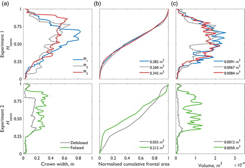
For the plants used in experiment 1, the crown width of Pl₁ differs from Pl₂ and Pl₃ (Figure 4(a)) with the maximum crown width ∼25% greater and positioned higher over H_norm. Differences in crown width are attributed to different branch architectures between the specimens. However, Figure 4(b) shows that although Pl₃ has the largest frontal area, ∼20% larger than Pl₁ and ∼30% larger than Pl₂, the curves for normalized cumulative frontal area are very similar between Pl₁, Pl₂, and Pl₃. For the vertical distribution of plant volume (Figure 4(c)), similarities in the volume distribution are shown between Pl₁, Pl₂, and Pl₃. The greatest degree of similarity in the distribution of volume exists between Pl₁ and Pl₃, although Pl₁ is volumetrically greatest (∼35% larger than Pl₂ and ∼10% larger than Pl₃). Plant geometric characteristics are shown to be similar between the foliated plants used in experiment 1, especially when the normalized cumulative frontal area and plant volume over H_norm are compared.

For the plant used in experiment 2 (Pl₄, defoliated and foliated), the lack of leaves for the defoliated plant considerably narrows the crown width (Figure 4(a)) and changes the overall flow-facing structure (Figure 4(b,c)). Beyond the main branching point (∼0.33 Z/h), the crown width of the foliated plant is approximately double that of the defoliated plant. Substantial differences are shown between the curves of normalized cumulative frontal area (Figure 4(b)) and volume over H_norm (Figure 4(c)). When defoliated, the curve for the normalized cumulative frontal area follows the line of equality more closely than for the foliated plant. Similarly, the defoliated plant volume is approximately equally distributed over H_norm, whereas for the foliated plant a marked increase in volume is associated with the leaf body beyond ∼0.33 Z/h. Overall, the total frontal area and the total volume of the defoliated plant is only ∼25% that of the foliated plant. Substantial differences in plant geometric characteristics are shown between the defoliated and foliated plant used in experiment 2.

A final comparison is made between the foliated plants in experiments 1 and 2. The foliated plants in experiment 1 (Pl₁, Pl₂, and Pl₃) are larger than the foliated plant in experiment 2 (Pl₄), having greater total frontal areas and total volumes. The distribution of crown width and plant volume over H_norm is displaced towards lower values for Pl₄ (Figure 4(a,c)). However, the normalized cumulative frontal area (Figure 4(b)) appears similar between Pl₁, Pl₂, Pl₃, and Pl₄. This is important as Pl₁, Pl₂, and Pl₃ are entire intact plants, whereas Pl₄ was a slightly smaller section pruned from a larger entire plant. This confirms similarities in the foliated plant geometry characteristics of entire plants and pruned sections.

Experiment 1: Flow field dynamics around three plants of the same species (Pl₁, Pl₂, and Pl₃)

To understand the flow field dynamics, first we present downstream (u–) velocity profiles at multiple locations in the model domain. Velocity profiles are shown at 0.30, 0.50, and 0.70 Y/w covering the downstream region 0.33, 0.40, 0.50, and 0.60 X/l (Figure 5) and normalized by the inlet velocity. To understand the average shape of velocity profiles, the mean normalized downstream velocity profiles from Pl₁, Pl₂, and Pl₃ are calculated. At each location in the model domain, the mean normalized downstream velocity profile is plotted alongside the normalized downstream velocity profiles for Pl₁, Pl₂, and Pl₃, thereby showing the range of velocity associated with the three plants.

Figure 5. Normalized downstream (u–) velocity profiles for Pl₁, Pl₂, and Pl₃ at (a) 0.30, (b) 0.50, and (c) 0.70 Y/w in the downstream region 0.33, 0.40, 0.50, and 0.60 X/l (locations shown as red dots in Figure 2). The upper text denotes the position of the velocity profile in the domain. The thick blue line represents the average downstream velocity profile, and the dashed grey lines indicate the minimum and maximum downstream velocities from Pl₁ to Pl₃ at each increment of Z/h. The filled grey area shows the range in downstream velocity for each profile. The lower text (grey) denotes the average range in downstream velocity, expressed as the normalized velocity, for each location in the domain.

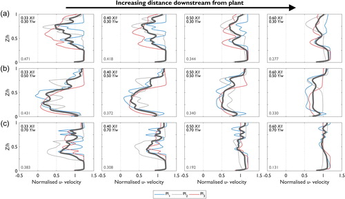
The mean normalized downstream velocity profiles show flow heterogeneity in the vertical direction (Z/h). Vertically, the three distinct velocity zones that were identified by Boothroyd et al. (2016a) are repeated here, with a zone of flow deceleration corresponding with the main plant body, and zones of flow acceleration above and beneath. However, a considerable range in the shape of normalized downstream velocity profiles is shown (fine lines for Pl₁, Pl₂, and Pl₃: Figure 5). When averaged over Z/h, the range in normalized downstream velocity between Pl₁, Pl₂, and Pl₃ at 0.33 X/l 0.30 Y/w is 0.471, equivalent to approximately 50% of the inlet velocity. At this location there is little variation in downstream velocity between Pl₁, Pl₂, and Pl₃ below 0.25 Z/h. However, above 0.25 Z/h, where flow begins to directly interact with the foliated plant body, a larger range in normalized downstream velocity is modelled (the maximum normalized range is 1.044 at 0.59 Z/h). For velocity profiles proximal to the plant (0.33–0.40 X/l), the range in normalized downstream velocity averaged over Z/h remains high (>0.3), although as flow recovers in the downstream direction (0.50–0.60 X/l) the magnitude of the normalized downstream velocity range reduces. The range in normalized downstream velocity and differences in velocity profile shapes between Pl₁, Pl₂ and Pl₃ indicate substantial differences in the downstream velocity field between the three P. laurocerasus plants.

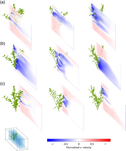
To understand more detail of the velocity field for Pl₁, Pl₂, and Pl₃, vertical slices of normalized downstream velocity at 0.30, 0.50, and 0.70 Y/w are taken (Figure 6). At the outer plant edges, the distribution of vegetal elements strongly influences flow field dynamics, specifically the shape of the decelerated velocity zone (<1, Figure 6(a,c)). Although the magnitude of normalized downstream velocity in these zones is similar, the position and size of the zone varies considerably between plants. This is shown at 0.30 Y/w, where Pl₃ has the largest decelerated velocity zone, forming when the plant is interacting more directly with the flow than for Pl₁ and Pl₂ (Figure 6(a)). At the domain midline, Pl₁ has the most substantial deceleration in the velocity zone immediately behind the plant body (Figure 6(b)). As shown in Figure 5, normalized downstream velocity is not constant over Z/h, and even within the decelerated velocity zone, flow heterogeneity is associated with changes in the distribution of vegetal elements. Although a decelerated velocity zone is formed behind Pl₃, this is limited to the region below 0.5 Z/h. Above this, a substantial zone of flow acceleration is shown (>1), where the localized region of faster moving flow is located between branch clusters. Vertical slices of the normalized downstream velocity field show that flow structures substantially differ between plants (e.g. between Pl₁ and Pl₃), indicating a unique flow disturbance from each plant.

Figure 6. Normalized downstream (u–) velocity field data for Pl₁ (column 1), Pl₂ (column 2), and Pl₃ (column 3). Slices at (a) 0.30 Y/w, (b) 0.50 Y/w, and (c) 0.70 Y/w are shown (see inset diagram for illustration of position in the numerical domain). The three-dimensional position of the plant is marked by the green shaded region.

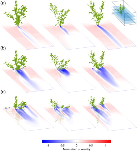
Further insights into the normalized downstream velocity field are provided by the horizontal slices at 0.10, 0.35, and 0.60 Z/h (Figure 7). The different perspective allows flow separation and reattachment around the plants to be identified. Similarity in the narrow zone of flow deceleration (<1) is shown about the main stem at 0.10 Z/h (Figure 7(a)). Beyond the main stem, the distribution of the vegetal elements changes due to the influence of the foliated plant body (Figure 4), and the flow disturbance becomes more complicated. The downstream extent of the decelerated velocity zones at 0.35 Z/h are shown in Figure 7(b). Here, the plants are more densely foliated, with the flow pattern response suggesting that the plants were behaving as a single foliated body, with the decelerated velocity zone constrained by the width of the plant. Differences exist where, in the downstream direction, the decelerated velocity zones extend further for the volumetrically larger plants (Pl₁ and Pl₃). As shown in Figures 2(b) and 4(a), over Z/h the distribution of vegetal elements and plant geometric characteristics change. As individual branches diverge in the upper canopy, the influence of isolated branches becomes more important. This is shown in Figure 7(c) for Pl₁ and Pl₃, where flow separates and reattaches around individual foliated branches, and so the decelerated velocity zones behave independently around these isolated elements. Together, Figures 6 and 7 indicate differences in flow structure in the normalized downstream velocity field from individual plants of the same species.

Figure 7. Normalized downstream (u–) velocity field data for Pl₁ (column 1), Pl₂ (column 2), and Pl₃ (column 3). Slices at (a) 0.10 Z/h, (b) 0.35 Z/h, and (c) 0.60 Z/h are shown (see inset diagram for illustration of position in the numerical domain). The three-dimensional position of the plant is marked by the green shaded region.

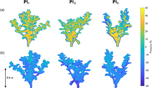
Results from the pressure fields are also investigated (Figure 8), allowing the form drag force (F_d) and drag coefficient (C_d) to be quantified (following Equations (1)(1) $$F_{\mathrm{d}}={\int }_A\left(p_{\mathrm{f}}-p_{\mathrm{b}}\right)d{A}_{\mathrm{p}}$$(1) and (2)(2) $$C_{\mathrm{d}}=\frac{F_{\mathrm{d}}}{\frac{1}{2}\rho u^2{A}_{\mathrm{p}}}$$(2) ). Similarity is shown in the spatial distribution of pressure on the upstream edge of the plants, with the zone of highest pressure consistently located just above the main branching point on each plant (Figure 8(a)). However, patterns of low pressure on the downstream edge are less clear (Figure 8(b)). The zones of lowest pressure are located towards the edges of the foliated branches in Pl₁ and Pl₃, but towards the main stem branch in Pl₂. Therefore, no consistent spatial pattern of low pressure acting on the downstream edge of the plants is shown.

Figure 8. Pressure distributions for Pl₁, Pl₂, and Pl₃ at (a) the plant front and (b) the plant back. This shows the similarity in the distribution of pressure between different plants of the same species, with highest positive and negative magnitudes of pressure distributed towards the lower region of the plant bodies.

Table 1 shows the considerable differences in plant drag response between Pl₁, Pl₂, and Pl₃. Total domain drag ranges from 7.03 to 9.84 N m² (variation of up to 40%), form drag ranges from 3.82 to 5.06 N m² (variation of up to 33%), skin friction drag for the whole domain ranges from 3.21 to 5.31 N m² (variation of up to 65%), and drag coefficients range from 1.38 to 1.81 (variation of up to ∼30%). Between Pl₂ and Pl₃, a 32% increase in plant frontal area and 25% increase in total plant volume causes a 33% increase in form drag. However, the drag coefficient appears insensitive to plant frontal area and total plant volume, as shown by Pl₃ which has the largest frontal area but the lowest drag coefficient (23% lower than Pl₁ and Pl₂). For each of the foliated plants, the values of form drag are of similar magnitude to the skin friction drag for the whole domain. Furthermore, variation is shown in the ratio of form drag to skin friction drag for the whole domain between plants, with the plant with the smallest frontal area and total volume (Pl₂) having the largest ratio. The drag response therefore differs between three plants of the same species, even though the plant geometric characteristics are largely similar.

Experiment 2: Flow field dynamics with changes in plant orientation and foliation

With 15° incremental changes in plant orientation, the shape of the normalized downstream (u–) velocity profiles proximal to the plant at 0.3 X/l 0.5 Y/w are modified (Figure 9(a)). Individual normalized downstream velocity profiles show heterogeneity over Z/h, with irregular profile shapes (e.g. 345° plant orientation in Figure 9(a)). When averaged over the 24 plant orientations (Figure 9(b,c)), the average normalized downstream velocity profiles become smoothed and the irregularity that was characteristic of individual profiles is obscured. With incremental changes in plant orientation, the changes in velocity profile shape for defoliated and foliated plants appear gradual. This is exemplified between 0° and 45° for the foliated plant in Figure 9(a), where at 0° the velocity profile shape is inflected and irregular but shifts towards a more linear velocity profile shape by a plant orientation of 45°. Beyond incremental changes, it is interesting to compare the shape of velocity profiles with a 180° change in plant orientation, as it is hypothesized that differences in the flow-facing structure of the plant to the incident flow should be minimized with a 180° change in plant orientation (Figure 3(b)). With a 180° change in plant orientation, the shape of the velocity profiles for some pairs of plants remain similar (e.g. 45° and 225°, 135° and 315°, both defoliated and foliated). However, there are notable exceptions where the shape of the velocity profiles substantially differ (e.g. the foliated plant at 0° and 180°). This difference is explained by the complex three-dimensional morphology of the plant which is not isomorphic. With vegetal elements asymmetrically distributed over the three-dimensional plant extent, a 180° change in plant orientation modifies the flow-facing structure of the plant, thereby influencing the presentation of the plant to incident flow and generation of flow structures.

Figure 9. (a) Normalized downstream (u–) velocity profiles at 0.30 X/l 0.50 Y/w for the defoliated (grey) and foliated (green) plants with changes in plant orientation, the average normalized downstream velocity profile for the (b) defoliated and (c) foliated plants, and the average frontal area and range of frontal area for the (d) defoliated and (e) foliated plants. In (b) and (c), the thick grey/green line indicates the average normalized downstream velocity profile and the dashed grey lines indicate the minimum and maximum normalized downstream velocities at each increment of Z/h. The filled grey area highlights the range in normalized downstream velocity using data from all 24 of the modelled plant orientations. Note the same axis ranges between (a) and (c). In (d) and (e), the thick grey/green line indicates the average frontal area and the dashed blue lines indicate the minimum and maximum frontal areas at each increment of Z/h. The filled blue area highlights the range in frontal area using data from all 24 of the modelled plant orientations.

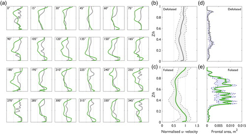
For the defoliated plant, the mean normalized downstream velocity profile (Figure 9(b)) shows a slight reduction from the inlet velocity (<1) around 0.4 Z/h. The velocity reduction appears to be associated with a small spike in frontal area (Figure 9(d)), although overall the distribution of frontal area appears approximately similar over Z/h, with only a narrow range with changes in plant orientation (shaded area, Figure 9(d)). Taking the minimum velocities for each of the 24 normalized defoliated velocity profiles, the mean normalized minimum velocity is 0.664, with a standard deviation of 0.076. The mean position of the velocity minima is 0.408 Z/h, with a standard deviation of 0.152 Z/h. The range in downstream velocity remains approximately consistent over Z/h.

For the foliated plant, a greater reduction in normalized downstream velocity is shown (Figure 9(c)). The reduction in velocity is greater than for the defoliated plant and this is associated with a marked increase in frontal area around the foliated body (∼0.4–0.8 Z/h, Figure 9(e)). Unlike for the defoliated plant, changes in the distribution of frontal area over Z/h are more substantial, with a larger range in frontal area identified with changes in plant orientation. The shape of the mean normalized downstream velocity profile for the foliated plant is more inflected. Taking the minimum velocities for each of the 24 foliated velocity profiles, the mean normalized minimum velocity is 0.492, with a standard deviation of 0.096. The mean position of the velocity minima is 0.598 Z/h, with a standard deviation of 0.164 Z/h. The range in downstream velocity over Z/h is less consistent than for the defoliated plant, with the largest velocity ranges shown in the near-bed region associated with sub-canopy flow (<0.25 Z/h), behind the lower half of the foliated body (∼0.4 Z/h) and in the flow acceleration zone above the canopy (>0.8 Z/h). The substantial range in downstream velocity behind the foliated body (Figure 9(c)) corresponds with the position where a large range in frontal area over Z/h was shown (Figure 9(e)) and this region is likely to be responsible for partitioning flow beneath/above the plant blockage.

Visually, the magnitude of the velocity reduction is greatest when plants are foliated (generally plotting to the left of the defoliated plant in Figure 9(a)). Comparing the results, the mean minimum velocity is lower for the foliated plant, with the velocity minima positioned higher in Z/h. This is associated with the distribution of plant frontal area over Z/h, specifically the presence of the foliated plant body. For the defoliated plant, the mean minimum velocity is higher, with the range in downstream velocities more consistent over Z/h. This is attributed to the smaller range in plant frontal area over Z/h with changes in plant orientation.

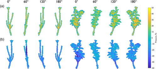
Differences in the pressure distributions over the plant bodies with 60° changes in plant orientation are shown in Figure 10. These increments were selected to show relatively larger (e.g. 0°–60°) and smaller (e.g. 0°–180°) changes in the flow-facing structure of the plant. For both the defoliated and foliated plants, changes in the plant orientation modify the pressure distributions on the plant front and plant back (Figure 10(a,b)). The largest differences are shown between plant orientations of 0° and 60°, where the defoliated and foliated plant shift from a more face-on alignment at 0° to a more edge-on alignment at 60°. For the defoliated plant at orientations of 0°, 120°, and 180°, a zone of relatively high pressure (>30 Pa) at the plant front is located on the main branching point. For the defoliated plant at 60°, the high pressure zone is displaced higher up the main stem. At the plant back, regions of relatively low pressure (<–30 Pa) are located along the main stem for all orientations, although the magnitude of the low pressure zone is greatest at a 60° orientation. The pressure gradient for the defoliated plant at a 60° orientation is ∼25% greater than the average pressure gradient of the plants at orientations of 0°, 120°, and 180°. For the foliated plant, the greatest similarities in the magnitude and distribution of pressure are shown at orientations of 0° and 180°, where the plant is aligned more face-on to flow. Relatively higher pressure on the plant front is positioned around the lower half of the leaf body (associated with the peak in frontal area in Figure 9(e)). Zones of lowest pressure are similarly positioned at the plant back. For plant orientations of 60° and 120°, where the plant is aligned more edge-on to the incident flow, the magnitude of high and low pressure is smaller and appears more evenly distributed over plant height. The average pressure gradient for plant orientations of 0° and 180° is 34% greater than the average pressure gradients for plant orientations of 60° and 120°. With changes in plant orientation, the differences in the spatial distribution and magnitude of pressure for the defoliated and foliated plant indicate that even small changes in flow-facing structure of the plant have a substantial influence on the pressure distribution.

Figure 10. Pressure distributions for the defoliated and foliated plants at plant orientations of 0°, 60°, 120°, and 180°. Pressure distributions at (a) the plant front and (b) the plant back. For both plants, pressure distributions are modified with changes in plant orientation (e.g. the position and magnitude of low pressure on the plant back changes between 0° and 60° plant orientations). The greatest similarity in pressure distribution is shown between 0° and 180°, when the plant is aligned more face-on to flow, and the flow-facing structure is more similar.

Form drag forces (F_d), drag coefficients (C_d), and frontal areas for each of the 24 plant orientations are quantified (Figure 11), with descriptive and directional statistics reported in Table 2. For the defoliated plant, the mean form drag force is 0.171 N m², with a standard deviation of 0.058 N m². Calculated form drag forces vary by up to ∼350%, ranging between 0.08 and 0.37 N m². For the foliated plant, the mean form drag force is 1.683 N m², with a standard deviation of 0.376 N m². Foliated form drag forces are approximately an order of magnitude greater, varying by up ∼130%, and ranging between 1.02 and 2.32 N m². For the defoliated plant, the mean drag coefficient is 1.520 with a standard deviation of 0.451. For the foliated plant, the mean drag coefficient is 1.033, with a smaller standard deviation of 0.172. Drag coefficients range from 0.95 to 2.92 for the defoliated plant (varying by up to ∼210%), but for the foliated plant the range is smaller, from 0.76 to 1.36 (varying by up to ∼80%). For both the defoliated and foliated plants, the drag coefficient tends to be greater than unity.

Figure 11. Effect of plant orientation on (a) form drag force, (b) drag coefficient, and (c) frontal area. Note the order of magnitude difference in form drag force between defoliated (grey) and foliated (green) plants. Clear axes of maximum and minimum symmetry are shown for the foliated plant, whereas discrete spikes in the drag response are shown for the defoliated plant. Directional statistics are shown in Table 2.

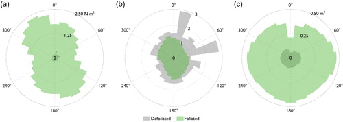
Table 2. Descriptive and directional statistics for the plant drag response (form drag and drag coefficient) for the 24 plant orientations in experiment 2 (Pl_{4 Def} and Pl_{4 Fol}).

Statistic			Form drag force		Drag coefficient
			Pl4 Def	Pl4 Fol	Pl4 Def	Pl4 Fol
Descriptive statistics	Mean	(N m^2/-)	0.171	1.683	1.520	1.033
	Standard deviation	(N m^2/-)	0.058	0.376	0.451	0.172
	Range	(N m^2/-)	0.282	1.304	1.970	0.602
Directional statistics	Mean	(°)	71.0	317.6	50.4	326.8
	Variance	(-)	0.895	0.991	0.900	0.995
	Angular deviation	(-)	1.338	1.408	1.342	1.410
	Circular skewness	(-)	–0.107	0.145	–0.055	0.095
	Circular kurtosis	(-)	0.030	0.022	0.019	0.054

Directional statistics quantify directional differences between the form drag force and drag coefficient for the defoliated and foliated plants over the entire range of plant orientations assessed. A key difference is shown, with the mean direction when defoliated (form drag force 71°; drag coefficient 50°) different than when foliated (form drag force 318°, drag coefficient 327°). Furthermore, Figure 11 shows clear axes of maximum and minimum symmetry for the foliated drag response, with the defoliated drag response characterized by a small number of discrete spikes. These differences are quantified through the circular variance, angular deviation, circular skewness, and circular kurtosis (Table 2). If drag response values were spread evenly around the circle, the circular variance would equal unity. For both the form drag force and drag coefficient, circular variance values are close to unity, however the value is consistently lower for the defoliated plant. The angular deviation is analogous to the linear standard deviation but bounded between 0 and $\sqrt{2}$ (Berens 2009). Angular deviation values for the defoliated plant are slightly lower than for the foliated plant, although both fall towards the upper bound. Circular skewness values for the foliated plant are slightly further away from 0, indicating less symmetry in the drag response around the mean direction for the foliated plant than for the defoliated plant. Finally, the similar values of circular kurtosis indicate that neither dataset are strongly peaked. Descriptive and directional statistics show differences in the drag response with changes in plant orientation, most notably in the different directionality in the drag response between the defoliated and foliated plants.

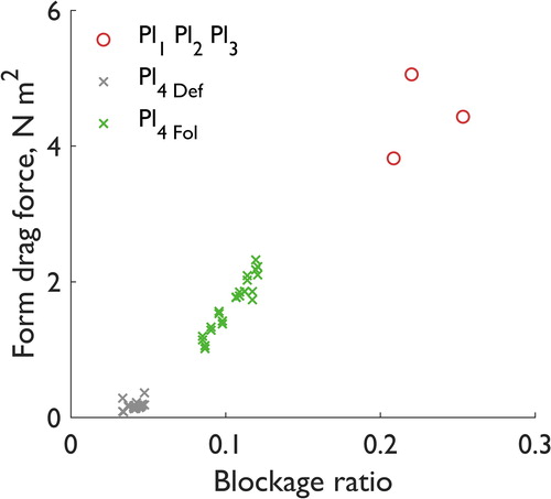
Finally, the control of blockage ratio on the form drag forces from experiments 1 and 2 are shown in Figure 12. In experiment 1, the blockage ratio varies by up to 21% from 0.209 to 0.253 across the specimens of the same species. In experiment 2, for both the defoliated and foliated plants the blockage ratio varies by up to 42% with changes in plant orientation (from 0.034 to 0.048 when defoliated; from 0.085 to 0.121 when foliated). Figure 12 shows that increases in the blockage ratio are associated with increases in the form drag force. This is likely to have important implications for the drag response when the plant width is of a similar order as the numerical domain width. Furthermore, the differences in blockage ratio between experiments 1 and 2 show the differences between entire intact plants (experiment 1) and pruned sections (experiment 2).

Figure 12. Blockage ratio effects on form drag force for different plants of the same species in experiment 1 (Pl₁, Pl₂, and Pl₃) and changes in plant orientation in experiment 2 (Pl_{4 Def} and Pl_{4 Fol}). Larger blockage ratios are associated with higher form drag force.

Discussion

Plant geometric characteristics were quantified from voxelized plant representations postprocessed from point clouds acquired by TLS. In experiment 1, the three foliated P. laurocerasus plants had similar distributions of cumulative frontal area and plant volume over normalized plant height, although total frontal area and total plant volume varied between specimens. However, in experiment 2 the defoliated plant had a distinct set of plant geometric characteristics from the foliated plant. For comparison with other species, Weissteiner et al. (2015) produced cumulative frontal area curves for 20 plant specimens including Alnus glutinosa, Betula pendula, Betula pubescens, and Salix caprea, all of which were harvested from a wetland in Finland. The specimens strongly differed in plant morphology and height (0.8–3.3 m), with smaller specimens (<2 m) showing an almost linear cumulative frontal area over normalized plant height, whereas the taller specimens showed a more pronounced increase in cumulative frontal area with normalized plant height. However, this size dependency was not shown for the Salix pentandra specimens investigated by Righetti (2008), finding similitude in the cumulative frontal area between smaller (0.7 m) and taller specimens (1.5–3.5 m) cut from the banks of restored mountain streams in the Trentino Region, Italy (Nobile 2007). Here we have shown that plants of the same species (P. laurocerasus) share similar geometric characteristics, particularly the distributions of cumulative frontal area and plant volume over normalized plant height.

However, the plant geometric characteristics likely differ between plant species, and this is related to their ecological functioning. Weissteiner et al. (2015) show that because Salix caprea is positioned close to riverbanks, and therefore inundated by frequent flooding, the branch architecture is adapted to reduce the frontal area at the tree base, thereby modifying the bending and drag response under hydrodynamic loading. In terrestrial environments, similar responses have been recorded where wind loading modifies the overall plant morphology over long timescales, producing “flagged” plants (Gardiner et al. 2016). These morphological modifications have important implications for flow field dynamics, which are influenced by a range of plant properties including: age, seasonality, foliage, areal, and volumetric porosities (Shields et al. 2017).

Results from experiment 1 show that differences in the distribution of vegetal elements have a considerable influence on the normalized downstream velocity field. Although the overall geometric characteristics were similar between the foliated P. laurocerasus plants, the modelled normalized downstream velocity fields differed. Each of the plants introduced a unique disturbance to the flow field, controlled by the branch architecture and position of the leaf body. Largest ranges in normalized downstream velocity were shown where the flow directly interacted with the foliated plant bodies, because the vertical and horizontal distribution of vegetal elements influence the velocity field (Lightbody and Nepf 2006). This has been shown previously for tamarisk plants (Tamarix chinensis/Tamarix ramossissima), where velocity profiles were nonmonotonic and inflected, with alternating zones of relatively slower and faster moving flow were associated with the plant body at different heights above the bed (Manners et al. 2015).

Results from experiment 2 show that with incremental changes in plant orientation, the shape of normalized downstream velocity profiles change. More specifically, the position and magnitude of the downstream velocity minima shift as the flow-facing structure of the plant is modified. This is explained by changes in the three-dimensional exposure of vegetal elements (Hurd 2000), with upstream elements extracting energy from the flow (Marjoribanks et al. 2014a), thereby providing a localized sheltering effect. These effects are largest for leafy plants (Takenake et al. 2010), and can cause a greater drag reduction in plants with multiple elements (complex branching structure) and higher leaf area (Jalonen et al. 2013). The differences in exposure and localized sheltering help to explain the differences in the normalized downstream velocity profiles, even between those plant orientations where there should be smaller differences in the flow-facing structure (e.g. 180° change in plant orientation). This is because the complex three-dimensional morphology of plants is not isomorphic and with vegetal elements asymmetrically distributed over the plant extent, changes in plant orientation modify the flow-facing structure of the plant and thus flow field dynamics. Results from experiment 2 show the importance of plant orientation on flow field dynamics and it is acknowledged that the initial orientation of Pl₁, Pl₂, and Pl₃ in experiment 1 would influence results presented here.

The highly heterogeneous normalized downstream velocity fields are analogous to the irregular shaped velocity profiles in channels with coarse bed roughness (after Byrd et al. 2000). Individual normalized downstream velocity profiles behind the plants appear irregular in shape, whereas the average normalized downstream velocity profiles appear more regular and smoothed (Figures 5 and 9). This is especially relevant where branches diverge, resulting in flow separation and reattachment about the individual branches, thereby influencing vortex shedding and controlling the types of coherent flow structures present in the region (Stoesser 2013). This raises the question to what extent can velocity profiles be generalized around morphologically complex plants, where the flow disturbance is dependent on the interplay between the three-dimensional distribution of vegetal elements and the orientation of the plant to the incident flow. Quantification of average velocity fields and profiles may obscure the local flow field dynamics that are unique to an individual specimen.

When considering the sensitivity of the pressure and drag response with changes in plant orientation, similarities are drawn with flow around impermeable, surface-mounted cuboidal blockages, positioned either face-on or edge-on to the incident flow. When face-on, a large portion of the kinetic energy in the incident flow is extracted through form drag. However, when the cube is edge-on, much of this kinetic energy is retained, with streamlines compressed and flow accelerated around the outside of the blockage (Lee and Soliman 1977). With the plant presented more face-on to the incident flow, this becomes analogous to a face-on cube, where the drag coefficient is greater than for the same cube positioned edge-on (face-on drag coefficient = 1.10; edge-on cube drag coefficient = 0.80; Streeter 1998). Visually, this was shown for the foliated plant by the axes of maximum and minimum symmetry in Figure 11. With the foliated plant presented more face-on to the incident flow, as shown at 0° and 180° in Figure 3, the pressure gradient was 34% greater than the average pressure gradients for plant orientations of 60° and 120°. This resulted in a larger form drag force and drag coefficient that were further investigated through directional statistics and showed the mean directionality of the drag response around a plant orientation of ∼320°.

Comparisons are also made with studies of large woody debris (LWD) in rivers that show trends in the drag coefficient with changes in tree log orientation (Gippel et al. 1996; Hygelund and Manga 2003; Shields and Alonso 2012). Measuring the drag response on cylindrical and tree-like models of logs in a laboratory flume, Gippel et al. (1996) showed that changes in tree log orientation have a large effect on the drag coefficient. For cylindrical logs the drag coefficients ranged from ∼0.4 to 1.2, whereas when trunks and branches were present, the drag coefficient varied less, from ∼0.35 to 0.65 (Gippel et al. 1996). For the branched model, the drag coefficients were lower because with the introduction of branches, the increase in drag force was less than the increase in frontal area. Conversely, field studies have shown a near constant drag coefficient with changes in the orientation of a cylindrical log (Hygelund and Manga 2003). However, these experiments were conducted over a hydraulically rough bed, thereby introducing irregular velocity profiles that are hypothesized to account for the differences from the work by Gippel et al. (1996). Shields and Alonso (2012) also introduced non-cylindrical branched logs into an outdoor grassed channel, with drag coefficients considerably influenced by log orientation. Drag coefficients ranged from 0.22 to 6.27 for the log orientations tested and corresponded with the drag coefficient values of 0.7 to 9.0 reported by Manners et al. (2007) for natural large wood formations. The findings from studies of large woody debris in rivers are comparable to the results from numerical modelling experiments reported here, with the orientation of the plant to the incident flow a primary control on the drag response.

Furthermore, when an impermeable surface-mounted cuboidal blockage is rotated from face-on to edge-on, the spatial patterns of erosion substantially change. In aeolian flows, McKenna-Neuman et al. (2013) show that when a cube is rotated to edge-on, fluid momentum increasingly spills around the blockage edges. This substantially extends and stretches vortex tails in the leeward direction, resulting in substantial erosion from the vortices that have formed (Sutton and McKenna-Neuman 2008; Bauer et al. 2013). When face-on, however, the spatial extent of erosion is smaller, with very limited erosion in the lee of the blockage. Significant variation in sediment removal has therefore been reported with changes in obstacle orientation. This is important for flow-vegetation interactions, where generation of a strong sub-canopy jet of fluid beneath foliated plants can induce significant bed scouring (Yagci and Kabdasli 2008; Yagci et al. 2016). Although the flow processes do not transfer directly from impermeable blockages to more permeable plant blockages, it is apparent that plant orientation does exert a control on flow field dynamics, has considerable implications for the drag response, and is expected to influence sediment transport processes.

In the current experiments, we acknowledge that variability has only been considered as morphological differences between specimens of the same species (experiment 1) and with rotation of a different specimen around the vertical axis (experiment 2). In natural rivers, flexible plants will reconfigure under hydrodynamic loading to reduce drag (Vogel 1994) resulting in further variability. Plant reconfiguration is a complex three-dimensional process, dynamically modifying the flow-facing structure of the plant to the incident flow. This involves shifts in the general plant posture due to static reconfiguration and streamlining to the mean flow (Sand-Jensen 2003; Siniscalchi and Nikora 2013) and dynamic reconfiguration associated with smaller scale oscillations to the instantaneous flow (Siniscalchi and Nikora 2013). Here, results have shown that small changes in the flow-facing structure have considerable implications for plant-scale flow structures and drag. Furthermore, results from experiment 2 suggest that changes in the flow incidence will influence flow field dynamics.

Our results showed that for the foliated plants, the magnitude of form drag was similar to the magnitude of skin friction drag for the whole domain. For riparian plant species, form drag usually dominates over skin friction drag (Nikora 2010; Västilä and Järvelä 2014). Where vegetation undergoes significant reconfiguration under hydrodynamic loading (e.g. macrophytes and blade-models of seaweed), form drag is assumed to be much smaller than skin friction drag (Nikora and Nikora 2007; Vettori and Nikora 2018). Furthermore, the contribution of form drag and skin friction drag varies as a plant reconfigures (Sand-Jensen and Pedersen, 2008; Whittaker et al. 2013). This is especially important for foliated plants, as foliage drag more directly relates to the exposed leaf area than to the foliage mass (Västilä and Järvelä 2014). At the leaf-scale, the orientation of individual leaves changes from perpendicular to parallel under hydrodynamic loading, leaf-scale drag therefore shifts from form drag to skin friction drag dominated (Vogel 1994). Further efforts to quantify the contributions of skin friction drag and form drag are needed, especially for full-scale riparian plants under hydrodynamic loading.

The current model presented here simulates a single plant on a plane bed and this limits transferability to natural river conditions. Both in-channel vegetation and riparian plants are seldom found in isolation, with the forces on individual plants reduced due to sheltering and through the reduced velocities in wakes from upstream plants (Sand-Jensen and Madsen 1992; Edwards et al. 1999). Cameron et al. (2013) and Biggs et al. (2016) showed that single patches of Ranunculus penicillatus cause appreciable flow alteration despite the background turbulence generated from gravel- and cobble-beds in the River Urie, Scotland. Marjoribanks et al. (2016) incorporated multiple vegetation patches and explicitly represented channel bed topography in a CFD model similar to that used here. The presence of vegetation increased small-scale flow variability but dampened the impacts of topographically induced flow recirculation. For multiple riparian plants on complex floodplain topography, the flow-facing structure of the plant is still likely to exert a control on the flow structures and drag response, with field/flume validation and further model development required to test this.

Practical implications of this research include the recommendation that future studies of flow–vegetation interactions at the plant-scale should explicitly consider and justify the flow-facing structure of the plant to the incident flow. This includes justification for the selection of individual plant specimens, and justification of how plants are positioned and orientated in the flume/numerical domain. As much as possible, these factors should reflect the plant in the natural prototype habitat. In terrestrial environments, wind loading is shown to shape overall plant morphology, with crown asymmetry an important acclimation response to windy environments (Gardiner et al. 2016), exposed plants tending to be smaller and more compact than sheltered plants (Telewski 1995) and windswept crowns having significantly lower drag (Telewski and Jaffe 1986). In aquatic environments, growth modifications and morphological changes (e.g. size reduction, changes in biomass allocation) are shown to occur in plants exposed to flow (Idestam-Almquist and Kautsky 1995; Coops and Van der Velde 1996; Puijalon et al. 2005). An appreciation of these factors is important when selecting plant specimens.

An additional practical consideration includes blockage ratio effects on plant-scale flow–vegetation interactions. Changes in plant orientation were responsible for up to 42% variation in the blockage ratio for individual plants (experiment 2) and increases in the blockage ratio were associated with increases in the form drag force (Figure 12). When plant width is of the same order as the flume width, this has previously been shown to influence drag acting on submerged macrophytes (Cooper et al. 2007). Where possible, it is suggested that sensitivity analysis be undertaken to understand the influence of blockage ratio effects, especially with changes in plant orientation. In practice, this could realistically be achieved by repeating at least one experiment/model run with the plant orientation modified by 90° to assess blockage ratio effects.

Results have shown that the calculated drag coefficients deviate substantially from the commonly assigned value of unity, or the typical drag coefficient value range from 1.0 to 1.2 that has been used to represent vegetation in hydraulic modelling applications (Dittrich et al. 2012). In experiment 1, the drag coefficient averaged 1.66 but ranged by ∼30% between Pl₁, Pl₂, and Pl₃. In experiment 2, the average drag coefficient across the 24 plant orientations for the defoliated plant (1.52) was larger than for the foliated plant (1.03), although the standard deviation for the defoliated plant was more than double that of the foliated plant. Considerable differences in drag coefficient between plants of the same species and with changes in foliation state are shown. Similarly, in flume experiments on branches of Salix viminalis, Salix alba, and Salix purpurea, Wunder et al. (2011) quantified drag coefficients in the range 0.35–0.85 when foliated and 0.5–2.0 when defoliated. The lower drag coefficients shown by Wunder et al. (2011), especially for the foliated plants, are explained by differences in the measurement technique (capturing actual plant projected area using underwater video compared with the pressure coefficient approach used here) and the influence of plant reconfiguration and streamlining to minimize drag in the flume experiments, compared with the rigid treatment in the CFD model. However, both studies show that a single drag coefficient value is unlikely to reflect the full range of plant morphologies for both individual and different plant species. This has practical relevance for riparian plants, where seasonal changes in the leaf-on and leaf-off morphology influence the drag response (Wilson et al. 2008; Whittaker et al. 2013).

For riparian species, previous work has shown that the flow structures and drag response vary with changes in foliation state and plant posture (Boothroyd et al. 2016a, 2017) and here we show the importance of the flow-facing plant structure. How the plant is “seen” by the incident flow and responds under hydrodynamic loading is therefore crucial, as differences in these factors result in a range of drag forces and drag coefficients. Drag force and drag coefficient parameterizations that rely only on a single plant morphology, or single hydrodynamic loading response, are unlikely to represent the full range of drag responses that even an individual species could exhibit. Future work should therefore: (i) seek to appreciate the ranges in the flow structure and drag response (both within and between species) and (ii) search for any commonalities in this response (both within and between species). If commonalities can be found (e.g. between similar species with similar morphological or reconfiguration traits), this might allow a move away from the need to provide high resolution simulations of flow–vegetation interactions at the plant-scale.

Conclusions

Results from a series of numerical modelling experiments demonstrate that individual submerged riparian plant specimens show substantial variation in the flow structure and drag response in river flow. For different specimens of the same species (experiment 1), and with incremental changes in plant orientation for foliated and mechanically defoliated plants (experiment 2), flow field dynamics have been quantitatively assessed. Key findings include:

1. Plant geometric characteristics are similar between foliated plants of the same species. Although branch architecture varies between foliated plants, influencing the three-dimensional distribution of vegetal elements (branches, stems and leaves), the cumulative frontal area, and distribution of plant volume are similar when these characteristics are normalized over plant height (Figure 4). With the foliage removed, the total volume of the defoliated plant is only ∼25% that of the foliated plant, and the volume is approximately equally distributed over plant height. For the foliated plants, the volume is less equally distributed over the plant height due to the presence of the leaf body.

2. Experiment 1 showed that different plants from the same species introduce unique flow disturbances. From normalized downstream velocity profiles taken proximal to three foliated plants, the average range in normalized downstream velocity is equivalent to ∼50% of the inlet velocity, indicating considerable differences exist between plants (Figure 5). The range is greatest above 0.25 Z/h, where flow directly interacts with the foliated leaf body. Velocity profiles are irregularly shaped (after Byrd et al. 2000) and analysis of horizontal and vertical slices of the normalized downstream velocity field indicate that the three-dimensional distribution of vegetal elements influences the flow field dynamics (Figures 6 and 7).

3. Experiment 2 showed that incremental changes in plant orientation result in gradual changes to the downstream velocity field, with the shape of velocity profiles and the position and magnitude of the velocity minima shifting as the flow-facing structure of the plant is modified (Figure 9). This is explained by changes in the exposure of vegetal elements (Hurd 2000), with localized sheltering effects introduced by the multiple vegetal elements and the foliated leaf body (Takenake et al. 2010; Jalonen et al. 2013). Conclusions (2) and (3) question the extent to which generalized velocity profiles can be quantified for morphologically complex plants, given that the irregularity characteristic of individual velocity profiles is obscured.

4. A substantial range of drag responses are quantified with changes in plant orientation; with form drag forces up to an order of magnitude greater for foliated than defoliated plants (Table 1, Figure 11). The mean drag coefficient for the defoliated plants (1.52) is larger than the mean drag coefficient for the foliated plants (1.03), although variation in the drag coefficients are greater when the plant is defoliated (up to ∼210% variation when defoliated, ∼80% when foliated). Likewise, for the three plants of the same species, drag coefficients range by up to 30%, from 1.38 to 1.81. Directional statistics showed that the mean direction of the drag response differed between defoliated and foliated plants (Table 2). With the foliated plant aligned more face-on to the incident flow, larger pressure gradients, form drag force, and drag coefficients were shown. The flow-facing structure therefore exerts a key control on flow field dynamics and the drag response. Newly quantified drag coefficients are generally greater than the previously established values used to describe vegetation in hydraulic modelling applications (C_d = 1.0–1.2; Dittrich et al. 2012), with a single drag coefficient value unlikely to reflect the full range of the plant morphologies and flow-facing structures for an individual riparian species (Figure 11).

Acknowledgments

Data used in this manuscript can be obtained by contacting the lead author. The authors are grateful to the Editor and two anonymous reviewers for providing helpful comments that have led to significant improvements in this manuscript.

Disclosure statement

No potential conflict of interest was reported by the authors.

Additional information

Funding

Richard J. Boothroyd was funded under NERC Doctoral Scholarship 1313876.

References

- Albayrak I, Nikora V, Miler O, O’Hare M. 2012. Flow-plant interactions at a leaf scale: effects of leaf shape, serration, roughness and flexural rigidity. Aquat Sci. 74:267–286.
- Anderson JD. 1984. Fundamentals of aerodynamics. New York (NY): McGraw-Hill.
- Bakry MF, Gates TK, Khattab AF. 1992. Field-measured hydraulic resistance characteristics in vegetation-infested canals. J Irrigat Drain Eng. 118:256–274.
- Bauer BO, Walker IJ, Baas ACW, Jackson DWT, McKenna-Neuman C, Wiggs GFS, Hesp PA. 2013. Critical reflections on the coherent flow structures paradigm in aeolian geomorphology. In: Venditti JG, Best JL, Church M, Hardy RJ, editors. Coherent flow structures at earth’s surface. Chichester (England): Wiley; p. 111–134.
- Béland M, Baldocchi DD, Widlowski J-L, Fournier RA, Verstraete MM. 2014. On seeing the wood from the leaves and the role of voxel size in determining leaf area distribution of forests with terrestrial LiDAR. Agric Forest Meteorol. 184:82–97.
- Berens P. 2009. CircStat: a matlab toolbox for circular statistics. J Stat Softw. 31:1–21.
- Bienert A, Hess C, Maas HG, von Oheimb G. 2014. A voxel-based technique to estimate the volume of trees from terrestrial laser scanner data. Int Arch Photogramm Remote Sens Spatial Inform Sci. XL-5:101–106.
- Biggs H, Nikora VI, Papadopoulos K, Vettori D, Gibbins C. Kucher M. 2016. Flow-vegetation interactions: a field study of ranunculus penicillatus at the large patch scale. In: Webb JA, Costelloe JF, Casas-Mulet R, Lyon JP, Stewardson MJ, editors. Proceedings of the 11th International Symposium on Ecohydraulics; 7–12 February; Melbourne (Australia). Melbourne (Australia): The University of Melbourne.
- Boothroyd RJ, Hardy RJ, Warburton J, Marjoribanks TI. 2016a. The importance of accurately representing submerged vegetation morphology in the numerical prediction of complex river flow. Earth Surf Process Landforms. 41:567–576.
- Boothroyd RJ, Hardy RJ, Warburton J, Marjoribanks TI. 2016b. Modelling vegetation-flow interactions: the importance of accurately representing plant morphology. In: Webb JA, Costelloe JF, Casas-Mulet R, Lyon JP, Stewardson MJ, editors. Proceedings of the 11th International Symposium on Ecohydraulics; 7–12 February; Melbourne (Australia). Melbourne (Australia): The University of Melbourne.
- Boothroyd RJ, Hardy RJ, Warburton J, Marjoribanks TI. 2017. Modeling complex flow structures and drag around a submerged plant of varied posture. Water Resour Res. 53:2877–2901.
- Bradbrook KF, Lane SN, Richards KS. 2000. Numerical simulation of three-dimensional, time-averaged flow structure at river channel confluences. Water Resour Res. 36:2731–2746.
- Byrd TC, Furbish DJ, Warburton J. 2000. Estimating depth-averaged velocities in rough-channels. Earth Surf Process Landforms. 25:167–173.
- Cameron SM, Nikora VI, Albayrak I, Miler O, Stewart M, Siniscalchi F. 2013. Interactions between aquatic plants and turbulent flow: a field study using stereoscopic PIV. J Fluid Mech. 732:345–372.
- Cooper GG, Callaghan FM, Nikora VI, Lamouroux N, Statzner B, Sagnes P. 2007. Effects of flume characteristics on the assessment of drag on flexible macrophytes and a rigid cylinder. N Z J Marine Freshwater Res. 41:129–135.
- Coops H, Van der Velde G. 1996. Effects of waves on helophyte stands: mechanical characteristics of stems of Phragmites australis and Scirpus lacustris. Aquat Bot. 53:175–185.
- de Langre E. 2008. Effects of wind on plants. Annu Rev Fluid Mech. 40:141–168.
- Disney MI, Boni Vicari M, Calders K, Burt A, Lewis S, Raumonen P, Wilkes P. 2018. Weighing trees with lasers: advances, challenges and opportunities. R Soc Interface Focus. 8:20170048.
- Dittrich A, Aberle J, Schoneboom T. 2012. Drag forces and flow resistance of flexible riparian vegetation. In: Rodi W, Uhlmann M, editors. Environmental fluid mechanics. London (UK): CRC Press; p. 195–215.
- Edwards PJ, Kollmann J, Gurnell AM, Petts GE, Tockner K, Ward JV. 1999. A conceptual model of vegetation dynamics on gravel bars of a large Alpine river. Wetlands Ecol Manag. 7:141–153.
- Ferguson RI, Parsons DR, Lane SN, Hardy RJ. 2003. Flow in meander bends with recirculation at the inner bank. Water Resour Res. 39:1322–1333.
- Folkard AM. 2016. Creating patches of comprehension and filling gaps in knowledge: physical modelling contributions to joined-up understanding of heterogeneous eco-scapes. In: Webb JA, Costelloe JF, Casas-Mulet R, Lyon JP, Stewardson MJ, editors. Proceedings of the 11th International Symposium on Ecohydraulics; 7–12 February; Melbourne (Australia). Melbourne (Australia): The University of Melbourne.
- Gardiner B, Berry P, Moulia B. 2016. Review: wind impacts on plant growth, mechanics and damage. Plant Sci. 245:94–118.
- Gippel CJ, O’Neill IC, Finlayson BL, Schnatz I. 1996. Hydraulic guidelines for the re-introduction and management of large woody debris in lowland rivers. Regul Rivers: Res Manag. 12:223–236.
- Hardy RJ, Lane SN, Ferguson RI, Parsons DR. 2003. Assessing the credibility of a series of computational fluid dynamic simulations of open channel flow. Hydrol Process. 17:1539–1560.
- Hardy RJ, Lane SN, Lawless MR, Best JL, Elliott L, Ingham DB. 2005. Development and testing of a numerical code for treatment of complex river channel topography in three-dimensional CFD models with structured grids. J Hydraulic Res. 43:468–480.
- Hess C, Bienert A, Härdtle W, von Oheimb G. 2015. Does tree architectural complexity influence the accuracy of wood volume estimates of single young trees by terrestrial laser scanning? Forests. 6:3847–3867.
- Hodskinson A, Ferguson RI. 1998. Numerical modelling of separated flow in river bends: model testing and experimental investigation of geometric controls on the extent of flow separation at the concave bank. Hydrol Process. 12:1323–1338.
- Hosoi F, Nakai Y, Omasa K. 2013. 3-D voxel-based solid modeling of a broad-leaved tree for accurate volume estimation using portable scanning lidar. ISPRS J Photogramm Remote Sens. 82:41–48.
- Hurd CL. 2000. Water motion, marine macroalgal physiology, and production. J Phycol. 36:453–472.
- Hygelund B, Manga M. 2003. Field measurements of drag coefficients for model large woody debris. Geomorphology. 51:175–185.
- Idestam-Almquist J, Kautsky L. 1995. Plastic responses in morphology of Potamogeton pectinatus L. to sediment and above sediment conditions at two sites in the northern Baltic proper. Aquat Bot. 52:205–216.
- Jalonen J, Järvelä J, Aberle J. 2013. Leaf area index as vegetation density measure for hydraulic analyses. J Hydraulic Eng. 139:461–469.
- Jalonen J, Järvelä J, Virtanen J-P, Vaaja M, Kurkela M, Hyyppä H. 2015. Determining characteristic vegetation areas by terrestrial laser scanning for floodplain flow modeling. Water. 7:420–437.
- Kadlec R. 1990. Overland flow in wetlands: vegetation resistance. J Hydraulic Eng. 116:691–706.
- Kouwen N, Unny TE, Hill H. 1969. Flow retardance in vegetated channels. J Irrigat Drain Div. 95:329–342.
- Lane SN, Hardy RJ, Elliott L, Ingham DB. 2002. High-resolution numerical modelling of three dimensional flows over complex river bed topography. Hydrol Process. 16:2261–2272.
- Lane SN, Hardy RJ, Elliott L, Ingham DB. 2004. Numerical modeling of flow processes over gravelly surfaces using structured grids and a numerical porosity treatment. Water Resour Res. 40:W01302.
- Launder BE, Spalding DB. 1974. The numerical computation of turbulent flows. Comput Methods Appl Mech Eng. 3:269–289.
- Lee BE, Soliman BF. 1977. An investigation of the forces on three dimensional bluff bodies in rough wall turbulent boundary layers. J Fluids Eng. 99:503–509.
- Lien FS, Leschziner MA. 1994. Assessment of turbulence-transport models including non-linear ring eddy-viscosity formulation and second-moment closure for flow over a backward-facing step. Comput Fluids. 23:983–1004.
- Lightbody AF, Nepf HM. 2006. Prediction of velocity profiles and longitudinal dispersion in salt marsh vegetation. Limnol Oceanogr. 51:218–228.
- Lilly DK. 1967. The representation of small scale turbulence in numerical simulation experiments. In: Goldstine HH, editor. Proceedings of IBM Scientific Computing Symposium on Environmental Sciences; 14–16 November; New York (NY). New York (NY): White Plains.
- Liu C, Zheng Z, Cheng H, Zou X. 2018. Airflow around single and multiple plants. Agric Forest Meteorol. 252:27–38.
- Luhar M, Nepf HM. 2011. Flow induced reconfiguration of buoyant and flexible aquatic vegetation. Limnol Oceanogr. 56:2003–2017.
- Manners RB, Doyle MW, Small MJ. 2007. Structure and hydraulics of natural woody debris jams. Water Resour Res. 43:W06432.
- Manners RB, Wilcox AC, Kui L, Lightbody AF, Stella JC, Sklar LS. 2015. When do plants modify fluvial processes? Plant–hydraulic interactions under variable flow and sediment supply rates. J Geophys Res Earth Surf. 120:325–345.
- Marjoribanks TI, Hardy RJ, Lane SN. 2014a. The hydraulic description of vegetated river channels: the weaknesses of existing formulations and emerging alternatives. Wiley Interdiscip Rev Water. 1:549–560.
- Marjoribanks TI, Hardy RJ, Lane SN, Parsons DR. 2014b. Dynamic drag modeling of submerged aquatic vegetation canopy flows. In: Schleiss AJ, Cesare G, Franca MJ, Pfister M, editors. Proceedings of River Flow 2014; 3–5 September, Lausanne (Switzerland). London (UK): CRC Press.
- Marjoribanks TI, Hardy RJ, Lane SN, Tancock MJ. 2016. Patch-scale representation of vegetation within hydraulic models. Earth Surf Process Landforms. 42:699–710.
- McBride M, Hession WC, Rizzo DM, Thompson DM. 2007. The influence of riparian vegetation on near-bank turbulence: a flume experiment. Earth Surf Process Landforms. 32:2019–2037.
- McKenna-Neuman C, Sanderson RS, Sutton SLF. 2013. Vortex shedding and morphodynamic response of bed surfaces containing non-erodible roughness elements. Geomorphology. 198:45–56.
- Moorthy I, Miller JR, Hu B, Chen J, Li Q. 2008. Retrieving crown leaf area index from an individual tree using ground-based lidar data. Can J Remote Sens. 34:320–332.
- Moorthy I, Miller JR, Berni JAJ, Zarco-Tejada P, Hu B, Chen J. 2011. Field characterization of olive (Olea europaea L.) tree crown architecture using terrestrial laser scanning data. Agric Forest Meteorol. 151:204–214.
- Naiman RJ, Décamps H. 1997. The ecology of interfaces: riparian zones. Annu Rev Ecol Syst. 28:621–658.
- Nepf HM, Ghisalberti M, White B, Murphy E. 2007. Retention time and dispersion associated with submerged aquatic canopies. Water Resour Res. 43:W04422.
- Nikora N, Nikora V. 2007. A viscous drag concept for flow resistance in vegetated channels. In: Di Silvio G, Lanzoni S, editors. Proceedings of the 32nd Congress of IAHR. Venice, Italy: Coirdila.
- Nikora V. 2010. Hydrodynamics of aquatic ecosystems: an interface between ecology, biomechanics and environmental fluid mechanics. River Res Appl. 26:367–384.
- Nikora V, Cameron S, Albayrak I, Miler O, Nikora N, Siniscalchi F, Stewart M, O' Hare M. 2012. Flow-biota interactions in aquatic systems. In: Rodi W, Uhlmann M, editors. Environmental fluid mechanics. London (UK): CRC Press; p. 217–235.
- Nobile, I. 2007. Dendrometric analysis of riparian vegetation in mountain streams [Ph.D. Thesis]. Trento (Italy): University of Trento.
- O’Hare MT, Mountford JO, Maroto J, Gunn IDM. 2016. Plant traits relevant to fluvial geomorphology and hydrological interactions. River Res Appl. 32:179–189.
- Oplatka M. 1998. Stabilität von Weidenverbauungen an Flussufern. Switzerland: Eidgenössische Technische Hochschule Zürich.
- Panton RL. 1984. Incompressible flow. New York (NY): Wiley.
- Petr T. 2000. Interactions between fish and aquatic macrophytes in inland waters: a review. Rome, Italy: UN Food and Agriculture Organisation. Fisheries Technical Paper 396.
- Pewsey A. 2004. The large-sample joint distribution of key circular statistics. Metrika. 60:25–32.
- Puijalon S, Bornette G, Sagnes P. 2005. Adaptations to increasing hydraulic stress: morphology, hydrodynamics and fitness of two higher aquatic plant species. J Exp Bot. 56:777–786.
- Riegl. 2015. Riegl laser measurement systems: Riegl VZ‐1000 datasheet. [accessed 2016 June 01] www.riegl.com/.
- Righetti M. 2008. Flow analysis in a channel with flexible vegetation using double-averaging method. Acta Geophys. 56:801–823.
- Rusu RB, Marton ZC, Blodow N, Dolha M, Beetz M. 2008. Towards 3D point cloud based object maps for household environments. Rob Auton Syst. 56:927–941.
- Sand-Jensen K. 1998. Influence of submerged macrophytes on sediment composition and near-bed flow in lowland streams. Freshwater Biol. 39:663–679.
- Sand-Jensen K. 2003. Drag and reconfiguration of freshwater macrophytes. Freshwater Biol. 48:271–283.
- Sand-Jensen K, Madsen T. 1992. Patch dynamics of the stream macrophyte, Callitriche cophocarpa. Freshwater Biol. 27:277–282.
- Sand-Jensen K, Pedersen M. 2008. Streamlining of plant patches in streams. Freshwater Biol. 53:714–726.
- Shields FD, Alonso CV. 2012. Assessment of flow forces on large wood in rivers. Water Resour Res. 48:W04516.
- Shields FD, Coulton KG, Nepf HM. 2017. Representation of vegetation in two-dimensional hydrodynamic models. J Hydraulic Eng. 143:1–9.
- Siniscalchi F, Nikora V. 2012. Flow-plant interactions in open-channel flows: a comparative analysis of five freshwater plant species. Water Resour Res. 48:W05503.
- Siniscalchi F, Nikora V. 2013. Dynamic reconfiguration of aquatic plants and its interrelations with upstream turbulence and drag forces. J Hydraulic Res. 51:46–55.
- Stoesser T. 2013. Calculation and education of coherent flow structures in open-channel flow using large-eddy simulations. In: Venditti JG, Best JL, Church M, Hardy RJ, editors. Coherent flow structures at earth’s surface. Chichester (UK): Wiley; p. 175–197.
- Stoesser T, Kim SJ, Diplas J. 2010. Turbulent flow through idealized emergent vegetation. J Hydraulic Eng. 136:1003–1017.
- Stone MC, Chen L, Kyle McKay S, Goreham J, Acharya K, Fischenich C, Stone AB. 2013. Bending of submerged woody riparian vegetation as a function of hydraulic flow conditions. River Res Appl. 29:195–205.
- Streeter VL. 1998. Fluid mechanics. New York (NY): McGraw-Hill.
- Sutton SLF, McKenna-Neuman C. 2008. Sediment entrainment to the lee of roughness elements: effects of vortical structures. J Geophys Res Earth Surf. 113:F02S09.
- Takenake H, Tanaka N, Htet PM, Yagisawa J. 2010. Wind tunnel experiments on direct measurement of drag force of real tree trunks and branches and their sheltering effects at high Reynolds numbers. Proceedings of the 8th International Symposium on Ecohydraulics; 12–16 September; Seoul (Korea). Seoul (Korea): Korea Water Resources Association.
- Telewski FW. 1995. Wind-induced physiological and developmental responses in trees. In: Coutts MP, Grace J. editors. Wind and trees. Cambridge (UK): Cambridge University Press; p. 237–263.
- Telewski FW, Jaffe MJ. 1986. Thigmomorphogenesis: field and laboratory studies of Abies fraseri in response to wind or mechanical perturbation. Physiol Plantarum. 66:211–218.
- Tempest JA, Möller I, Spencer T. 2015. A review of plant-flow interactions on salt marshes: the importance of vegetation structure and plant mechanical characteristics. Wiley Interdiscip Rev Water. 2:669–681.
- Thomas RE, Johnson MF, Frostick LE, Parsons DR, Bouma TJ, Dijkstra JT, Eiff O, Gobert S, Henry P, Kemp P, et al. 2014. Physical modelling of water, fauna and flora: knowledge gaps, avenues for future research and infrastructural needs. J Hydraulic Res. 52:311–325.
- Tritton DJ. 1988. Physical fluid dynamics. Oxford (UK): Clarendon Press.
- Västilä K, Järvelä J. 2014. Modeling the flow resistance of woody vegetation using physically based properties of the foliage and stem. Water Resour Res. 50:229–245.
- Vettori D, Nikora VI. 2018. Flow-seaweed interactions: a laboratory study using blade models. Environ Fluid Mech. 18:611–636.
- Vierling KT, Vierling LA, Gould WA, Martinuzzi S, Clawges RM. 2008. Lidar: shedding new light on habitat characterization and modeling. Front Ecol Environ. 6:90–98.
- Vogel S. 1994. Life in moving fluids: the physical biology of flow. Chichester (UK): Princeton University Press.
- Watts JFW, Watts GD. 1990. Seasonal change in aquatic vegetation and its effect on channel flow. In: Thornes JB. editor. Vegetation and erosion. Chichester (UK): Wiley; p. 257–267.
- Weissteiner C, Jalonen J, Järvelä J, Rauch HP. 2015. Spatial–structural properties of woody riparian vegetation with a view to reconfiguration under hydrodynamic loading. Ecol Eng. 85:85–94.
- Whittaker P, Wilson C, Aberle J, Rauch HP, Xavier P. 2013. A drag force model to incorporate the reconfiguration of full-scale riparian trees under hydrodynamic loading. J Hydraulic Res. 51:569–580.
- Wilson C, Hoyt J, Schnauder I. 2008. Impact of foliage on the drag force of vegetation in aquatic flows. J Hydraulic Eng. 134:885–891.
- Wilson CAME, Stoesser T, Bates P, Pinzen A. 2003. Open channel flow through different forms of submerged flexible vegetation. J Hydraulic Eng. 129:847–853.
- Wunder S, Lehmann B, Nestmann Franz. 2011. Determination of the drag coefficients of emergent and just submerged willows. Int J River Basin Manag. 9:231–236.
- Yagci O, Celik MF, Kitsikoudis V, Ozgur Kirca VS, Hodoglu C, Valyrakis M, Duran Z, Kaya S. 2016. Scour patterns around isolated vegetation elements. Adv Water Resour. 97:251–265.
- Yagci O, Kabdasli MS. 2008. The impact of single natural vegetation elements on flow characteristics. Hydrol Process. 22:4310–4321.
- Yakhot V, Orszag S. 1986. Renormalization group analysis of turbulence. I. Basic theory. J Sci Comput. 1:3–51.
- Zar JH. 1999. Biostatistical analysis. Upper Saddle River (NJ): Prentice Hill.