Turbulent eddy identification of a meander and vertical-slot fishways in numerical models applying the IPOS-framework

Abstract

Fishways are an important link for the reestablishment of river continuity, interrupted by transverse structures e.g. weirs, dams and hydropower plants. The meander fishway and vertical slot fishway are two types commonly constructed in Germany, which create distinctive flow regimes to allow upstream passage. Nonetheless minor environmental or constructional alterations create unforeseen flow regimes, whose impact on fish behaviour is still uncertain. One approach is to obtain different flow aspects for fish by evaluating numerous parameters with the IPOS-framework in laboratory experiments. The framework provides various identification parameters and methods, which must be considered with regard to fish behaviour. This paper expands the experimental approach by using numerical simulations with OpenFOAM on one meander and two vertical slot fishways and employs the evaluation methods stated in the IPOS-framework. The results shows clear differences between the fishways, providing an advanced numerical evaluation method to objectively compare turbulent flows in the models. The 3D-hydronumerical evaluation of 1:1 scaled fishways using the IPOS-framework is a novelty so far and can be used to improve present and future fishway constructions.

Keywords:

• Fishways
• river continuity
• IPOS
• 3D-simulation
• OpenFOAM

1. Introduction

The European Water Framework Directive (WFD) requires all member states of the European Union to achieve a “good status” for all surface and groundwater bodies by 2027 at the latest (European Community 2000). While the “good status” is subdivided into “ecological status” and “chemical status”, this study deals solely with the “ecological status” of surface water bodies. In 2016, only 8.2% of Germany’s surface water bodies achieved a “good ecological status” (BMUB/UBA 2016). In order to increase this percentage, ecosystem criteria have to be improved, e.g. the abundance and age structure of fish fauna. Due to a lack of available habitats and migration corridors in river systems, the fish fauna have deteriorated, which is one of the main reasons for the unsatisfactory ecological status (BMUB/UBA 2016). Therefore, restoring a stable fish fauna is an important step towards achieving a “good ecological status”.

River continuity plays an important role for developing a stable fish fauna. The river connectivity is disrupted at traverse structures, such as dams and weirs. To overcome this discontinuity, fishways are constructed, which allow up- and downstream migration of fish (Fehér et al. 2012). The meander fishway and the vertical slot fishway are two types of fishways currently being constructed in Germany. These two types have been analysed in the past with in-situ and physical as well as numerical models (Musall et al. 2014; Stamm et al. 2015a; Lohnstein 2016).

With the help of national guidelines for fishway construction parameters, engineers have a first reference point during the planning stage. For example, the existing German guideline DWA-M509 for the construction of fishways sets threshold values for specific fish regions like the maximum flow velocity or the specific power density $p_D.$ It depends on the basin volume, basin drop height and discharge, but lacks information on how the flow regime inside the basin influences fish behaviour. One reason is the omitted insight regarding turbulent eddy structures. Another point is the low number of evaluation parameters, which are simple to obtain but overlook further turbulent parameters (DWA 2014).

The IPOS-framework emerged from a study that tried to unite strain-relevant parameters for fish by dividing them into categories, explicitly the intensity (I), periodicity (P), orientation (O) and scale (S) of the prevalent turbulent flow (Lacey et al. 2012). It states different parameters and investigation procedures for each category and gives a structured way to comprehend present flow and turbulence characteristics.

To date, no attempt has been made to model both the meander and the vertical slot fishway, using the same numerical software with a suitable evaluation method to compare those flow parameters. The meander fishway was selected due to its clear separation of main flow near the basin wall and calm recirculation pool around the basin centre, while the two vertical slot fishways were designed to generate either a straight or strongly diverted main flow throughout each basin, as explained in further detail in section 2. By applying the same numerical software and the IPOS-framework, an objective comparison between the fishways is possible. By employing the same turbulence model, boundary conditions and mesh procedures, the numerical differences between the simulation models are minimised. The flow regimes in all fishways are then analysed and compared with each other with the IPOS-framework. Accordingly, the different flow systems within the fishway and high-turbulent regions are distinguished and located. In addition, the 3D-hydronumerical model allows for a unsteady time-dependent calculation, visualisation, and comparison of eddy structures generated by these fishways, which is a novelty so far.

Hence, the objectives of this study are to (1) investigate turbulent variables in different fishway designs using the IPOS framework, (2) numerically identify and quantify turbulent eddies and (3) assess critical differences between designs of construction.

2. The fishways

The fishways under study belong to the pool-shaped fishways in which water flows from one basin to the next through vertical slots overcoming the transverse-structure water surface level difference. Within each basin, the energy head is reduced. Besides the common vertical slot fishway with rectangular shaped pools (Figure 1(b,d)), the meander fishway forms another type of construction, which is characterised by near three-quarter circle-shaped pools (Figure 1(a,c)).

Figure 1. Explanatory illustrations of the MF and the VSF. The bold white arrows in the sub-figures point in the flow direction. (a) Photo of a MF located on the Nethe river near Höxter, Germany. Source: Stamm et al. (2015a); (b) Photo of a VSF located on the Mosel river near Koblenz, Germany; (c) Aerial side view of the MF CAD model; (d) Aerial side view of the VSF 30°CAD model.

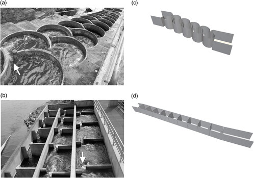
The meander fishway (MF) developed by Peters Fischpass Ökologie is an assembly of overlapping near three-quarter circles, which are connected through vertical slots (Peters 2004). The name originates from the distinct meandering flow that occurs within the MF. The flow is guided along the basin walls through the basin and the energy head is reduced within each basin. At the centre of each basin a steady and slow recirculation pool is present. Therefore, the basic flow pattern is described with these distinctive regions The meandering pattern has been demonstrated with physical modeling on several vertical slot design a while ago (see Rajaratnam et al., 1992). Recent studies have shown that the flow pattern inside the MF is stable and does not vary with basic geometric design alterations, e.g., radius, slope or discharge (Stamm et al. 2015b; Lohnstein 2016; Jähnel 2017).

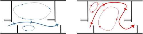
The vertical slot fishway (VSF) is a channel divided into single basins by long baffles with attached baffle blocks and short baffles (Figure 1(b,d)) (Wu et al. 1999). Vertical slots over the entire water height connect the basins. A water jet forms after the slot and its energy is dissipated through mixing within the basin (Wu et al. 1999). First studies evaluating the hydraulics of VSF showed that the geometric design of the basins influences hydraulic parameters and the overall shape of the water jet (Rajaratnam et al. 1986). Nowadays, two main flow patterns are described in the literature to categorise commonly-constructed VSF (Wu et al. 1999; Wang et al. 2010; Musall et al. 2014). In flow pattern 1, a slightly curved main jet develops from one slot to another, with eddies forming on each side of the jet. It leaves two recirculation zones, one on the opposite wall of the slot entrance and a smaller one at the near wall side. In flow pattern 2, a strongly curved jet develops that flows towards the wall furthest away from the slot, before curving back towards the downstream slot (Figure 2). A recirculation pool is present on the upstream slot side of the basin (Wu et al. 1999). While flow pattern 2 in a VSF may resemble the meandering flow in the MF (Rajaratnam et. al. 1992), the flow charactersics were never put against each other.

Figure 2. Display of two main flow patterns within VSF basins. (a) Flow pattern 1, where the main flow goes straight from the upstream to the downstream-located slot; (b) Flow pattern 2, with a redirected main flow to the opposite side of the wall.

Until now, determination of overall flow patterns in VSF relied on physical modeling (e.g. Wu et al. 1999). Various laboratory studies highlight prediction methods by looking at the length/width ratio of each basin, slot width, slot angle, discharge or slope of the basin’s bottom to decide the overall flow pattern. It is also known that geometric combinations exist where the flow patterns alternate between each basin. Minor inflow or geometric variations can be used to establish a fixed flow pattern in such cases (Musall et al. 2014; Höger et al. 2015; Bombač et al. 2017). Based on this, two VSF variations in an unstable region are taken into consideration to analyse the influence of the two flow patterns. The desired flow pattern is formed by varying the placement of the short baffle block inside the basin.

This study considers three different fishway designs overall: one MF and two VSFs, which are recommended by DWA (2014) for e.g., brown trout, creek chub, grayling and roach. All fishways comprise nine basins with a total drop height of 1.50 m between the upstream and downstream bed level. The drop heights are distributed equally by a constant bottom inclination, leading to a total of ten drops of 0.15 m level difference between the upstream basin entrance and downstream basin exit. The slot width for all fishways is 0.20 m. The discharge was set to Q = 200 L/s. As this work serves as an example emphasising the enhancement of the IPOS methodology with a numerical approach, further variations of design parameters or discharge were not investigated.

The MF was designed with a radius of 0.70 m and a slot angle of γ = 65°, leading to the three-quarter-circle design (MF 65°). The bottom slope between the upstream entrance of the first basin and the downstream exit of the last basin result in a slope degree of 11.6° (20,83% slope). This resembles the constructed fishway located on the Nethe river near Höxter, Germany (Stamm et al. 2015a). The Höxter MF also serves as a reference design, because it was verified with previous experimental data.

The VSFs have a basin length of 2.00 m and width of 1.60 m. Therefore, the bottom slope degree between the entrance and exit of the fishway is 4,76° (8,3% slope). The only difference between the two VSFs is the slot angle, which varies between γ = 30° and γ = 45°. This design forms either flow pattern 1 or an indeterminable flow pattern, depending on the evaluation methods given by Höger et al. (2015) and Musall et al. (2014). By changing the slot angle γ in each basin, a clarification of flow pattern was realised, with γ = 30° (VSF 30°) forming flow pattern 1 and γ = 45° (VSF 45°) flow pattern 2. These slot angles are characteristic boundary values for VSF constructions as stated in the German guidelines (DWA 2014). The main constructional design parameters for all fishways are depicted in Figure 3.

Figure 3. Illustration of the different basin designs constructed with slot width of b = 0.20 m. (a) Dimensions of the MF constructed, with the method to obtain a basin angle of γ = 65° according to Stamm et al. (2015a); (b) Overall dimensions of the VSF basin with varying length at the diversion baffle. Measurements in unit meters.

3. Numerical approach

OpenFOAM 5.0 and its interFoam solver for two incompressible, isothermal immiscible fluids using Volume-Of-Fluid (VOF) phase-fraction-based interface capturing was applied for the hydro numerical two-phase simulation (air, water) (Greenshields 2015). The three CAD fishway models were meshed with OpenFOAM v1712 or v1906, which provided the third-party tool cfMesh (v 1.1). The usefulness and implementation of OpenFOAM along with the interFoam solver for hydraulic engineering applications (e.g., fishways) has been shown in various previous studies (Schulze and Thorenz 2014; Duguay et al. 2017; Gisen et al. 2017). To exclude influences from up-/downstream lying basins and boundary conditions, a simulation of the entire fishway is mandatory. Since the whole domain is calculated, a flawless mesh in agreement with a Large-Eddy-Simulation, that captures all eddies larger than the mesh refinement while modelling smaller ones (Gramlich 2012; Gritskevich et al. 2012) is preferable but not feasible due to the high computational demand. Therefore, a deviation in optimal meshing parameters is necessary.

A compromise was achieved by using a hybrid turbulence model known as Detached-Eddy-Simulation. It employs the less computationally demanding and steady-state Reynolds-Average-Navier-Stokes-Simulation (RANS) near the walls (Rodi 2017) and a Large-Eddy-Simulation (LES) in the main flow region. This turbulence model requires small cell sizes near the walls in the boundary layer of the model and a larger of constant size in the main flow (Spalart 2001; Rodi 2017). The RANS is used to model the steady state and mainly viscous flow of the boundary layer in the fine meshed wall regions. As soon as the simulation models spread outside the boundary layer, a LES turbulence model is applied, which requires a constant cell size throughout its domain and calculates all eddies larger than or equal to its cell size. The LES results in turbulent and unsteady flows and is mandatory to investigate IPOS parameters. Without the split of the boundary and main flow area, a pure LES would require a fine and equal cell size throughout the whole domain, thus increasing the computational costs manifold. extent. The LES quality is now dependant on the choice of cell refinement in the main flow, as the LES turbulence closure is no longer coupled to the boundary layer (Spalart 2001; Gramlich 2012). The specific DES turbulence model used in this study is the Spalart-Allmaras-Improved-Delayed-Detached-Eddy-Simulation (SA-IDDES) (Spalart 2009; Gritskevich et al. 2012), which fitted well with previous experimental studies of fishways at TU Dresden (Stamm et al. 2015b; Jähnel 2017; Schneider 2017).

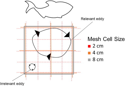
Given the turbulence model and its advantages, all fishway models are meshed in the same way to reduce numerical differences. In order to identify relevant vortex structures, a Cartesian mesh with an overall edge length of 0.02 m discretises the whole domain. This size was chosen to keep the computational costs as low as possible, while retaining fish-relevant eddies. Those high-intensity and relevant eddies are the size of a fraction of the smallest fish body measurements (Lacey et al. 2012; Silva et. al. 2012). A common size for an average roach is between 10 cm and 30 cm (Tudorache et al. 2008), where the relevant body fraction for the minimum mesh refinement would be around one-third of the fish’s (smallest) body measurement. The presented mesh in this study is smaller than the fish-relevant eddy for this example, therefore we assume it is of sufficient detection quality according to the principle of a LES. While a spinning region of fluid described by one computational cell does not guarantee an eddy with high confidence, additional refinement increases the certainty of those eddy structures, as can be seen in Figure 4. In order to demonstrate the evaluation method, we chose an exemplary minimum fish measurement of 4.6 cm (body length of a juvenile roach) to evaluate the swimming capacity stated in the discussion in section 6. The chosen cell size therefore suffices in this study.

Figure 4. Sketch of the correlation between the relevant fish size, eddy diameter and cell size. More cells describe a connected region of fluid (upper right eddy), improving its identification and visualisation. Eddies smaller than the cell size will not be captured and thus will not be relevant in the evaluation.

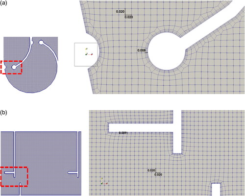
An additional boundary-layer was constructed uniform in proximity to the wall faces, with three prismatic cells growing in size towards the main flow region. The first prismatic layer thickness amounts to roughly 1 mm and expands inwards with a factor of 1.5 until three layers are constructed, leading to a total thickness of the boundary-layer-cells of ≈0.02 m with a maximum first-layer thickness of ≈0.0025 m. With this, we achieved a non-dimensional wall spacing of y⁺ ≈ 10-30, depending on the calculation approach and estimated mean flow, that describes the distance and region near the wall according to the boundary-layer theory (CFDyna 2015; Schlichting and Gersten 2017). The first layer cell is located in the buffer-region or lower-log-region which is outside of the recommended viscous region for the SA-IDDES turbulence model of y⁺ < 1 (Wilcox 2010; CFDyna 2015; Schlichting and Gersten 2017; Roth 2019). Nonetheless, we expect the mean values to be lower inside the whole domain, which cannot be accounted for beforehand due to recirculation flow near the slot regions and additional correction parameters for the dimensional wall distance implemented in the SA-IDDES turbulence model (Gramlich 2012; Roth 2019). The application of wall functions in this case is not suitable, since the recirculations induce a backflow, which cannot be accounted for with this method (ANSYS, Inc. 2014). The meshing parameters lead to a total cell count between ≈4.5 M (MF) and ≈6.5 M (VSF). The cfMesh tool proved to be a stable and easy-to-use meshing environment while satisfying all requirements to employ the SA-IDDES. In Figure 5, a horizontal 2D slice through the domain is depicted for the MF and VSF 45 °, showing an excerpt of the constructed mesh in basin 5 and a magnification near the slot region (red-marked area), where the boundary layer construction near the basin baffles can be seen.

Figure 5. Horizontal 2D-slice through the domain, showing an excerpt of the constructed mesh in basin 5 and a magnification near the slot region (marked area) for the MF (a) and VSF 45° (b).

After defining the turbulence model and overall mesh parameters, the boundary conditions can be set accordingly. The boundary conditions throughout all simulations are identical, since meshing and hydraulic boundary conditions match throughout all variations. This allows a numerical comparison between all simulated fishway variations.

Since the inflow rate is set to 200 L/s at the inlet, the upstream water level is calculated through the variableHeightFlowRate boundary condition during simulation. The outlet holds the water level at ≈0.65 m with a free flow condition by using the prescribed boundary conditions shown Table 1 for the outlet and translating by intended outlet water surface level to z = 0 m. The solver requires additional parameters for a SA-IDDES, such as the dissipation rate $\epsilon ,$ the turbulent kinetic energy $k$ (TKE) and the viscosity-equivalent variable $\mathit{nuTilda}$ on the boundary faces (Inlet/Outlet/Top/Basins) to initialise the simulation. The calculation method for these values follows the instructions in the OpenFOAM user manual (Greenshields 2015) and Gramlich (2012).

Table 1. Boundary conditions applied in OpenFOAM for all simulation faces.

Name/Type	alpha.water	U	p_rgh	k	epsilon	nuTilda
Inlet	variableHeightFlowRate	variableHeightFlowRate	zeroGradient	fixedValue	fixedValue	fixedValue
(patch)		0.2		0,24	1.61	0,18
Outlet	inletOutlet	pressureInletOutletVelocity (0 0 0)	totalPressure	inletOutlet	inletOutlet	zeroGradient
(patch)	0		0	0.00414	4.39E-05
Top	inletOutlet	pressureInletOutletVelocity (0 0 0)	totalPressure	inletOutlet	inletOutlet	zeroGradient
(patch)	0		0	0.00414	4.39E-05
Basins	zeroGradient	fixedValue	zeroGradient	fixedValue	fixedValue	fixedValue
(wall)		(0 0 0)		0	1.00E-20	0

Note: Due to similar meshing parameters, they are used for every fishway variation. Calculation methods are described in Greenshields (2015) and Gramlich (2012).

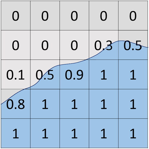
An advection equation implemented with an indicator function alpha.water (α) is used to track the position and shape of the interface (Greenshields 2015): $$\frac{\partial \alpha }{\partial t}+\nabla \left(\overrightarrow{v}\mathrm{ }\alpha \right)+\nabla \left({\overrightarrow{v}}_r\mathrm{ }\alpha \mathrm{ }\left(1-\alpha \right)\right)=0$$

Essentially, one phase is given the value of 1 (water) and the other phase the value of 0 (air). Thus, cells with a mixture of both phases have values between 0 and 1. The water surface interface can be resolved by extracting cells with a value close to α = 0.5. However, the interface can be computationally smeared. Thus, the finer the mesh within the region of the phase interface, the better the interface will be resolved with greater accuracy, as it can be seen in Figure 6 (Schneider 2017). Since the general computational mesh size is set at 0.02 m, the accuracy to pinpoint the water surface level is equal. An overview of all initial boundary conditions is given in Table 1.

Figure 6. Schematic visualisation of the VoF interface in a Cartesian mesh. Cells filled with water show α = 1, with air α = 0. Values between 0 < α < 1 are partially filled and define the water surface.

4. Evaluation methodology: the IPOS-framework

Turbulent flows can be decomposed into a variety of parameters, whereupon the IPOS-framework was proposed as a means to categorise, quantify and discuss the interaction between fish and turbulence (Lacey et al. 2012). The framework states for each category – namely intensity (I), periodicity (P), orientation (O) and scale (S) – detection and calculation methods for laboratory or field experiments to evaluate the strains on fish. The results are then linked to existing research on swimming capacity. In this paper, the IPOS methodology is applied to the simulated fishways, while expanding the method with numerical techniques not stated in the original paper to objectify and simplify the evaluation of turbulent flow.

Beginning with the intensity category, the velocity magnitude $u$ and vorticity $\omega$ hold major importance to estimate strains on fish induced by turbulent flows. The average of both parameters gives a first impression of fatiguing impacts that a fish would experience, but instantaneous fluctuations and direction changes must also be considered since a sudden increase of values (bursts) can destabilise fish (Tritico and Cotel 2010). While the flow velocity $u$ is a commonly-used threshold criterion to assess the functionality of fishways, the vorticity $\omega$ – which describes how fast a region of fluid is spinning around a certain point – is often neglected. Previous experiments with brown trout by Tritico and Cotel (2010) showed that eddies with low vorticity had no effect, while higher vorticity ones led to body rotations and destabilisation. While assessing turbulent flows, vorticity therefore plays a central role in quantifying the turbulent eddy structures.

The periodicity category focuses on the frequency of various-sized eddies in the turbulent flow. Lacey et al. (2012) mention energy spectral analysis as a means to estimate the predictability of turbulent eddies. Additional research has shown that with increasing Reynolds numbers, the strict periodicity of shedding eddies after bluff bodies starts to decrease until it turns non-periodic (Blevins 1990; Williamson 1996). As both methods require advanced data evaluation methods in laboratory experiments, we suggest a new approach to this category by filtering only high-intensity eddies from the remaining flow. A periodic pattern of those eddies could encourage upwards swimming for fish even in high-turbulent flows, since adapting body motions along those eddies reduces energy consumption (Liao et al. 2003). By contrast, similar laboratory experiments show that a non-periodic shedding frequency indicates higher energy consumption and destabilisation of fish (Enders et al. 2003; Tritico and Cotel 2010). The first step is to identify those high-intensity eddies, which is complex in laboratory studies since a dense probe raster is necessary to capture them. Nonetheless, the numerical mesh constructed for the simulations with a constant Cartesian cell size of 0.02 m grants a sufficiently dense probe grid. It can identify fish-relevant eddy structures in terms of detail and scale. The simulation parameters chosen in this study enable using different vortex identification criteria to filter those relevant eddies.

One method to calculate and visualise eddies of different intensities is given by the Q-criterion (Holmén; Hunt et al. 1988; Holmén 2012). It is a vortex criterion that requires solely the velocity components of the flow at each numerical cell, meaning that it can be evaluated in retrospect to already-completed simulations, as long as the mesh fulfils the discretisation requirements for the scope of evaluation. The Q-criterion value $Q$ is calculated by the following equation: $$Q=\frac{1}{2}\left[{\left(\nabla \cdot \mathit{u}\right)}^2-tr\left(\nabla \mathit{u}2\right)\right]$$

It describes the local balance between the shear strain rate and vorticity magnitude, where a positive Q-criterion value highlights that the vorticity magnitude is greater than the magnitude of the rate of strain (Hunt et al. 1988; Holmén 2012). Negative values indicate a translatory flow and no spinning. The Q-criterion therefore sets the velocity and the vorticity magnitude in relation, displaying fast-rotating eddy “hulls” or vortex cores inside the flow (Hunt et al. 1988). An issue is the choice of a threshold value to isolate relevant eddies, which must be set subjectively according to the present flow.

After filtering the relevant eddies, their orientation can be determined by the direction of their vorticity magnitude tensor. If the eddy orientation inside the basins is not clearly periodic or morphs, the vortex structure should be visually inspected. A simplification is possible, where the direction of the main eddies is clear, e.g., eddies swirling mainly around the z-axis. They have a positive vorticity z-component, spinning counter-clockwise, and vice versa. The evaluation of the eddy orientation is of essence when taking the body shape or fin arrangement of fish into account. Eddies with sufficient high-intensity values combined with an unfavourable orientation generate additional strain to specific fish species (Enders et al. 2003; Cotel et al. 2006; Tritico and Cotel 2010).

The scale category distinguishes further relevant eddies affecting fish behaviour. As eddy sizes span from the Kolmogorov microscale to many times the depth, only a small spectra pose a difficulty for fish (Nikora et al. 2003; Tritico and Cotel 2010). Various laboratory experiments have concluded that disturbing eddies are approximately a fraction between two-thirds to three-quarters of the fish’s body length (Pavlov et al. 2000; Tritico and Cotel 2010; Silva et al. 2012). In terms of evaluation, Lacey et al. (2012) focus on the eddy length scale and eddy diameter. Both values can be obtained spatially with the introduced vortex identifier, but they require advanced evaluation methods in the three-dimensional spectra. Their complexity increases as soon as the eddy’s shape starts to bend, while passing through parts of the probes. Therefore, we chose to focus on predefined transects and compare the overall size distribution visually with the data obtained.

5. Results

5.1. Steady-state flow and probes

After a simulation time of t = 100 s, all three fishway variations reached a stationary state, where the water surface elevation does not significantly change. The mean flow depth for the MF basin centre lies around 0.85 m. At the outer wall region of the MF, higher water levels can be observed due to its constructional design, which guides the flow along the basin perimeters. The VSF water level fluctuates around 0.75 m over the basin centre. The water levels as well as the velocities correlate with previously-validated simulations and research conducted at the Institute of Hydraulic Engineering and Technical Hydromechanics (IWD) (Jähnel 2017; Schneider 2017). The results for the evaluation are subsequently obtained for 10 s (tstart = 100 s, tend = 110 s) at an interval of 25 Hz (0.04 s), leading to 251 time steps for one simulation variation. Each time step requires ≈0.8 GB of disc space overall, while only relevant evaluation data (velocity, vorticity, $Q,$ $\alpha$) amounts to ≈0.5 GB. The total amount of disc space per fishway was 200 GB (total) or 125 GB (evaluation data). The mesh information takes up ≈1.5 GB of disc space for each fishway.

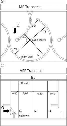
For the evaluation, three transects are defined: the first lying shortly after the upstream slot, the second in the middle of the basin length, and the third being shortly before the downstream slot, as shown in Figure 7. On these transects, probe locations at a distance of ≈0.02 m (MF) or ≈0.05 m (VSF) were defined. The boundary layer cells are omitted in the following transect evaluations. By focussing on the middle-located basin no. 5 of each fishway, the flow pattern identification and IPOS evaluation is conducted to exclude up- and downstream boundary condition influences (Stamm et al. 2015b). The transects were obtained on different water levels above the basin centre bed level (e.g., VSF: 0.175 m | 0.425 m | 0.675 m), but reduced to the transect horizon at 0.425 m on the first transect T1 in all variations, since the upstream slot region possesses the highest velocities and supposedly also the strongest strain on fish. Considering that the transects T2 and T3 revealed lower flow intensity overall – as can be seen in the appendix files¹ – they will be used to verify the numerical model as shown in the discussion, but neglected in the evaluation section to keep the overview. Also a water level diagram for each fishway is availiable in the appendix, since the fluctuations can be neglected for this evaluation.

Figure 7. Transect placement inside the MF and VSF fishways. The probe distance is defined in both cases from the right side wall to the centre point/left wall of the basin. (a) Transect placement inside the MF basins; (b) Transect placement inside the VSF basins.

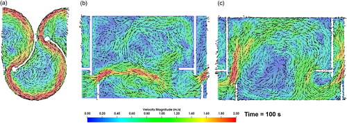
The flow patterns inside the basins demonstrate clear differences between the fishways, as seen in Figure 8. The main flow inside the MF is guided along the basin walls from one slot to another, with a recirculation pool spinning slowly around the basin centre. Flow pattern 1 prevails in the VSF 30° simulation, while it changes to flow pattern 2 in the VSF 45° simulation as intended.

Figure 8. Slice through basin 5 visualising the flow pattern and velocities of the MF (a), VSF 30° (b) and VSF 45° (c). All sub-figures show a snapshot at the simulated time step $t\mathrm{ }=\mathrm{ }100\mathrm{ }s.$

5.2. Evaluation of the fishways as proposed by the IPOS-framework

5.2.1. Intensity

The boxplot diagram shown in Figure 9 provides a statistical overview of the velocity magnitude through all time steps. It shows the median and interquartile ranges for all probes set in transect T1. Figure 10 shows the vorticity magnitude ${\omega }_{mag}$ in an identical way.

Figure 9. Boxplots of the velocity magnitude $U_{mag}$ for basin 5 in the MF (a), VSF 30° (b) and VSF 45° (c).

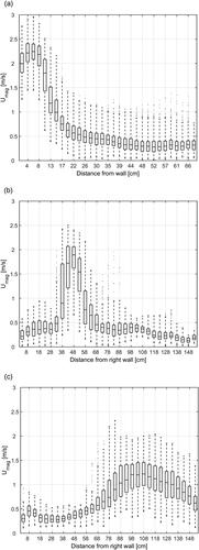
Figure 10. Boxplots of the vorticity magnitude ${\omega }_{mag}$ for basin 5 in the MF (a), VSF 30° (b) and VSF 45° (c).

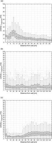
The MF simulation shows high average (median) velocities between 1.75 m/s and 2.25 m/s near the basin wall, which drop to 0.25 − 0.50 m/s near the basin centre. The fluctuations shown by the extent’s interquartile range indicate a wide range near the wall up to 0.5 m/s, decreasing to 0.25 m/s inside the recirculation pool. The vorticity magnitude is the highest among the fishways, with an average of up to 25 1/s at the shear zone and an interquartile range of between 13 1/s to 32 1/s. Looking at the outliers (upper and lower 25% of the values), the vorticity in this zone shows a wide range between almost 0 1/s to 65 1/s. The vorticity steadily decreases towards the basin centre.

In the VSF 30° case, a rapid and highly fluctuating velocity is seen near the main flow between ≈0.40 and 0.65 m away from the right side wall. The highest average velocities are around 2.0 m/s, with fluctuations between 0.75 m/s and 1.00 m/s around the main flow zone. Inside the recirculation zones, the average velocities drop to ≈0.25 m/s, with fluctuations ranging from 0.25 − 0.1 m/s. The average vorticity magnitude along the transect appears to be equally distributed along the transect, with an average of between 5 1/s and 10 1/s. The interquartile range goes up to 15 1/s, while strong outbursts of up to 40 1/s can be seen at some probes.

The VSF 45° case displays average velocities between 1.00 m/s and 1.25 m/s on the left side of the basin due to flow pattern 2, with widespread fluctuations around ≈0.50 m/s. On the basin’s right side, those values drop significantly to ≈0.25 m/s for the average and 0.1 m/s for the fluctuations. In terms of the vorticity magnitude, a similar distribution is seen. The average vorticity is between 10 1/s and 12.5 1/s at the left side of the basin, with an interquartile range between 7 1/s and 19 1/s. The right side of the basin shows noticeably lower vorticity values.

5.2.2. Periodicity

Figure 11 shows a boxplot of the Q values at each probe in transect 1. Figure 12 visualizes the MF variation for basin 5 and the respective spinning eddy hulls. The minimum threshold value was set to $Q>150\frac{1}{s^2},$ after inspecting the flow data visually. This was also suited for the VSF 30° and VSF 45° data, as seen in Figure 13.

Figure 11. Boxplots of the Q-criterion for basin 5 in the MF (a), VSF 30° (b) and VSF 45° (c).

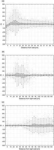
Figure 12. Eddies (grey) extracted from basin 5 under the entire water surface (light blue) of the MF at t = 100 s, shown from an isometric view (orientation axis lower-left corner). The eddy shedding starts directly after the upstream slot and does not change its rotation axis inside the basin.

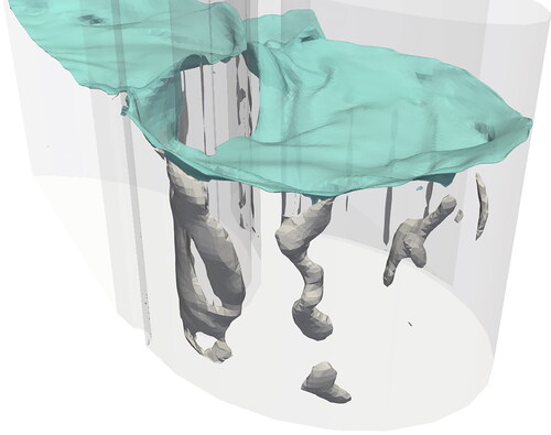
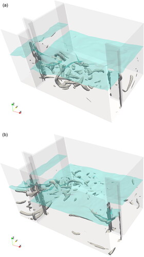
Figure 13. Eddies (grey) extracted from basin 5 under the entire water surface (light blue) of the VSF 30° (a) and VSF 45° (b) at t = 100 s, shown from an isometric view (orientation axis lower-left corner). The eddy shedding starts directly after the upstream slot. The rotational axis changes drastically inside the basin (hairpin vortices).

By isolating the stronger spinning vortices in the main flow, a respective frequency of high-intensity eddies is visible throughout the time steps. By employing the $Q$ threshold, we can quantify the largest eddy passing at a time step through transect T1, as seen in Figure 14, with the grey line and the left axis showing its diameter in the horizontal (x-y) plane. In addition, the black dots coupled with the right axis shows the distance between the eddy centre and the outer (MF) or right (VSF) wall side of the basins.

Figure 14. Eddy-Signal-Diagram showing the simulation time (bottom axis), diameter (left axis – line) and location (right axis – dots) of the largest passing eddy on transect 1 in the MF (a), VSF 30° (b) and VSF 45° (c).

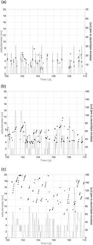
Throughout the 10 s observation frame, the MF shows an almost periodic eddy shedding in the near wall zone. The eddies spawn one by one near the slot, pass at transect T1 with a spread of ≈0.20 m and are of similar size, as further discussed in the scale category.

The VSF 30° shows two distinctive eddy zones, one being between 0.30 − 0.50 m and the other 0.60 − 0.80 m away from the right side wall. The eddy sizes differ during the observation time and are difficult to predict. A frequency derivation in this case is futile, since multiple different-sized eddies can be present at the same time step in the transect.

The VSF 45° has a widespread high-intensity eddy zone on the left side of the basin. In this case, a frequency is difficult to obtain due to multiple eddies at the transect. A clear eddy shedding pattern in the VSF simulations could not yet be obtained by data or visually, due to the rotational complexity and amount of the eddies described in the following orientation category.

5.2.3. Orientation

The visualisation of vortices in Figure 12 and Figure 13 at the timestep t = 100 s, enables a first visual impression of the orientation in each fishway. The eddies in the MF basin 5 emerge through all time steps uniformly spinning counter-clockwise around the z-axis, with a high positive z-vorticity component. This is confirmed by taking a look at the z-vorticity component, as shown in Figure 15 with boxplots. These counter-clockwise vertical-spinning eddies exist in every odd-numbered MF basin (left diverting flow), while even-numbered basins (right diverting flow) spin clockwise, having negative z-vorticity components.

Figure 15. Boxplots of the vorticity z-component for basin 5 in the MF (a), VSF 30° (b) and VSF 45° (c). It can be seen that in the MF boxplot the mathematical sign mainly remains in the positive range. The VSF 30° switches its sign at ≈50 cm away from the right wall and therefore its spin orientation around the z-axis changes.

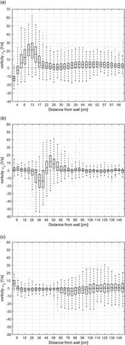
The VSFs display constant morphing eddies in the main flow area. They develop at a short distance after the upstream slot and deform/dissipate into hairpin vortices, whose spinning direction changes throughout the eddy length. It is worth mentioning an observation in the VSF 30° where the eddy orientation switches. A look at the z-vorticity component in Figure 15 shows an alteration in orientation over all time steps, due to which the mathematical sign changes between ≈45 and ≈50 cm away from the right wall, which coincides with the main flow region. This means that eddies on the two sides of the main flow spin differently from one another. In the VSF 45°, no orientation pattern was visible with current methods.

5.2.4. Scale

The diameter of an eddy is calculated by counting the intensity criteria satisfying cells consecutively and multiplying them by the cell size (0.02 m) along the transect. In Figure 14, the grey line and left axis display the largest eddy passing through transect T1 at any given time.

For the MF, the high-intensity eddies pass near the main flow region with constant eddy sizes between 4 cm and 8 cm. An eddy (axis) length is also accessible due to the uniform geometry, by comparing/adding transects at different heights.

In the VSFs, the eddy diameter ranges between 4 cm and 16 cm, being twice as large compared with the MF. An evaluation method for eddy lengths shaped as hairpin vortices is difficult, since they stretch outside of the transect line. Advanced evaluation methods and further research needs to be conducted to obtain eddy lengths in these cases.

6. Discussion

6.1. General statements

The procedures suggested in the IPOS-framework by Lacey et al. (2012) are suited to objectively identify complex flow and turbulence parameters in numerical models. An appropriate comparison can be made for different fishways or hydraulic structures in an objective and streamlined procedure.

The MF displays a uniform flow pattern throughout the whole evaluation. Almost every parameter of the IPOS-framework shows that its turbulent features are easier to grasp numerically since flow guides design and construction. The velocity and vorticity magnitudes are the highest among the observed fishway designs. As fish wander upstream, they would encounter high-turbulence eddies near the main flow, with a near periodic frequency, orientation and size inside each basin.

The VSF 30° variation establishes a strong lead current from the upstream- to the downstream-located slot. It displays flow pattern 1 throughout the whole fishway, as previously estimated by Höger et al. (2015) and Musall et al. (2014). The dominant eddies are in the shape of a hairpin developing after the slots with their switching spinning directions depending on the side of the main flow, which is a distinctive feature of this design. The eddy shedding has a noticeable constant periodicity and remains inside the main currents boundaries.

The VSF 45° creates a recirculation flow inside the basin, leading to flow pattern 2. The eddies forming inside basin 5, shaped like hairpin vortices, are on average smaller in size and have in general the lowest maximum intensity. They spread widely in the left side of transect T1. Since not only the frequency but also location of the eddies is important for a periodic flow, this variation seems to be the most unpredictable. A major orientation pattern of the eddies is not visible.

The flow patterns obtained in the simulations correspond to previous research and should not be omitted regarding flow regime stability inside fishways (Musall et al. 2014; Höger et al. 2015; Stamm et al. 2015b). Until now, the topic of the best flow regime inside fishways is highly discussed. This study proves that with even a slight constructional change, the flow pattern can switch, given that the construction lies in an unstable design region (Musall et al. 2014). Looking at the presented IPOS evaluation and the flow patterns of each fishway, we assume that there are missing aspects of the framework as well as guidelines for design and construction to assess the functionality of fishways for the prevalent fish species.

6.2. Comparison of fish swimming capacity and IPOS evaluation

6.2.1. Intensity

From a fish’s perspective, the passability of a fishway is measured by its own swimming capacity against the prevalent flow. The flow velocity combined with metabolic measurements or video-tracking footage of fish serve as a main indicator to assess the swimming capacity of the flow. The swimming capacity varies depending on the fish species, water temperature and bodily dimensions (Tudorache et al. 2008). The fishways investigated are designed in accordance with German guidelines for brown trout, creek chub or roach (DWA 2014). The results from Tudorache et al. (2008) state critical flow velocities for juvenile roach between 0.45 m/s and 0.60 m/s, which are exceeded at some places inside the simulated fishways. Adult specimens of roach presented a critical flow velocity with an average of 1.11 m/s. Similar evaluations by Tritico and Cotel (2010) specified the critical velocity for creek chub on average at around 0.53 m/s, which decreased in the presence of turbulent eddies to 0.41 m/s − 0.47 m/s. We assume that juvenile roach and creek chub will avoid the near wall region of the MF, which had the highest velocities between the three fishways. Adult roach would experience similar difficulties as their juvenile counterparts, since the velocities in the shear flow region increase drastically. Nonetheless, all specimens have the chance to pass through at the inner half of the slot width (≈10 cm − 20 cm from the outer wall), which exerts velocities in their capacity range. The remaining basin of the MF would serve as a recreational area, where the max flow velocities for roach do not exceed 0.30 m/s to 0.42 m/s on average. A similar resumé could be given for the VSF 30° case. On the other hand, the VSF 45° is suspected to be the most exhausting for juvenile roach as they encounter statistically higher flow velocities compared with the fish’s critical velocity at the left half of the basin. This is contrary to the initial impression that we would expect looking at the velocity boxplot diagram of the VSF 45° case. By contrast, adult roach are expected to pass the VSF 45°.

6.2.2. Periodicity

In case individual fish encounter difficulties achieving a successful passage, they would try to compensate by adjusting their swimming path or strategy. They could to either exploit the high energy vortices by adjusting their locomotion to incoming eddies or seek refuge in near wall or bottom areas, where flow velocities are usually lower (Gerstner 1998; Webb 1998; Liao et al. 2003; Liao 2007; Tudorache et al. 2008). The numerical approach chosen in this study allows us to identify both mechanisms simultaneously, especially the observation of time dependent turbulent eddies.

The identification of high-turbulent eddies through the vorticity $\omega$ serves as a first indicator. The high-vorticity eddies were obtained within the simulations and are essential for identifying the periodicity, orientation and scale aspects of the IPOS-framework. In their experiments, Tritico and Cotel (2010) acquired higher vorticity measurements with increasing flume velocity, e.g., having a vorticity of $\omega$ = 3 s⁻¹ at $u$ = 0.1 m/s velocity or ω = 12 s⁻¹ at u = 0.5 m/s. Since the vorticity is dependent on the surrounding velocity, this parameter must be set in comparison with the main flow by using vortex criteria to obtain a relation to the prevalent flume velocity. Therefore, the eddy identification with the vorticity is subjective in our case, since it is velocity dependent and should be adjusted with experimental as well as numerical data for each fishway design and fish species.

This leads to the proposal of the Q-criterion as an eddy identifier of numerical evaluations in this study, which is not yet stated in the IPOS-framework. It helps to identify relevant vortex structures by defining eddies as areas where the vorticity magnitude is greater than the magnitude of the rate-of-strain (Holmén 2012). A prerequisite of this method is a dense probe raster to identify the eddy structures. Since the framework sources mainly laboratory and field experiments – where the identification of eddy structures usually has a coarse probe raster – numerical models overcome this drawback. The numerical mesh required in our DES/LES simulations is finer than the magnitude of the relevant eddy scale of commonly-researched fish species (Tritico and Cotel 2010; Pavlov et al. 2000; Silva et al., 2012). A sensitive matter in this evaluation is the threshold for a high-intensity eddy structure using the Q-criterion. For the MF simulation, strong eddy structures were obvious and corresponded well with high vorticity values, especially in the shear zone between the main flow and recirculation pool. With a vorticity threshold of $\omega >25\mathrm{ }{s}^{-1},$ the eddies in the MF resembled those obtained with a threshold of $Q>1501/s^2.$ As the MF and VSF share the same boundary and mesh conditions, the threshold of $Q>1501/s^2$ provided the best agreement of high-turbulent eddies through all variations. To identify possible swimming capacity thresholds using the Q-criterion for different fish species, additional laboratory research with live fish is of essence.

6.2.3. Orientation

In terms of fishway performance, the simulations show clear differences regarding the orientation of eddies, assuming that some species would have difficulties. If we compare the influence of this category – e.g., from the perspective of a roach against a creek chub – inside the MF the cross-sectional body shape in each plane would play a crucial role (Lacey et al. 2012). As we have constant high-intensity eddies that spin mainly in the z-direction, the roach – with its rather deep body compared with its length – would experience a greater impact in comparison with longitudinally-oriented creek chub. Since both fish species demonstrate similar swimming capacity in terms of intensity (DWA 2014; Tudorache et al. 2008; Tritico and Cotel 2010), the MF geometric design yields at first sight a hydraulic barrier for the roach, induced by its constant horizontal-spinning eddies. Nonetheless, it could also have the adverse effect of benefitting the performance of the roach, in case it could use the eddies to propel itself forward by adjusting its body to the periodic eddy shedding that it produces. In addition, we expect the horizontal-spinning eddies in the MF to not benefit or even influence the swimming pattern of species similar to rainbow trout or creek chub (Liao et al. 2003; Lacey et al. 2012).

Since the VSF demonstrated no primary spinning direction, we assume that they would not exclude any fish species, solely due to the orientation of eddies.

6.2.4. Scale

The effects induced by the orientation are highly dependent on the other categories of the IPOS-framework, especially when taking the scale of the eddies into account. Some research suggests that the most severe impacts on fish are observed, when the eddies have the size of a major fraction of the fish’s dimensions (Pavlov et al. 2000; Tritico and Cotel 2010; Silva et al. 2012), while small or very large eddies impose little to no effect. As the size and orientation of eddies hold major importance to distinguish their relevance, we want to put usual body shapes and dimensions of a fish species in the context of the evaluated fishways (Cada and Odeh 2001; Lacey et al. 2012). In reference to the roach evaluated by Tudorache et al. (2008), with body lengths of 4.6 cm, 7.3 cm (juvenile) and 15.7 cm (adult) on average, we can presume the possible effect of the eddy sizes inside each simulated fishway. In the MF, the expected eddy sizes between 4 cm to 8 cm would mainly affect the juvenile individuals. We assume that adult species with a ratio of body/eddy-ratio ≈0.5 would still be affected by the eddies, as the orientation is disadvantageous looking at their body shape. In the VSF cases, the variety of eddy sizes increases up to 16 cm, implying that roach in all life stages would be affected by the identified eddies.

6.2.5. Summary

Summarising the IPOS-evaluation for all fishways exemplary for a roach, we can state the following conclusions:

• Intensity: Juvenile roach should pass the MF and VSF 30° fishways, while the VSF 45° poses a difficulty due to the high velocities spread at transect T1. Adult specimen are able to pass all variations.

• Periodicity: The frequency of the shedding eddies is difficult to appraise but seems predictable. The orientation of the eddies in the MF is constant. Additionally, the location of the emerging eddies and high flow velocities are apparent in the MF and VSF 30° case, which could help roach to compensate for other IPOS parameters. The VSF 45° is chaotic and decreases the fishway’s functionality in this category.

• Orientation: The constant horizontal-spinning eddy in the MF could create ambiguous effects for roach depending on the size and age of the individual. For the dominant hairpin vortices in the VSF, no statement can be made yet.

• Scale: The dominant eddy sizes will have an impact on roach, because the typical body lengths correspond to the critical body-eddy ratios mentioned in all fishway variations.

Providing a definitive ranking of the most suitable fishway for all roach specimen based on the IPOS-framework would be far-fetched without additional research and improvement of the evaluation method. Apart from focussing the evaluation on hydraulic parameters, we suggest conducting additional strain measurements of the fish’s condition with numerical methods on the presented fishways, which could be validated with laboratory experiments using the fish shaped artificial-lateral-line-probe (Tallin University of Technology 2018).

6.3. Numerical limitations and future improvements

As this study relies on numerical models, the validation and verification of results holds utmost importance. Since we chose the smallest computational possible fish-relevant eddy as the maximum cell size (2 cm), a grid convergence study would further assure the numerical integrity. One way to ensure this is to refine the mesh iterative to the point where no differences in the results are visible, reflecting numerical convergence. A common and acknowledged procedure for estimating such errors is the Grid Convergence Index (GCI) based on the method described by Celik et al. (2008). It requires additional simulations of the same model with a coarser and finer numerical mesh. In the meshing process we encountered a computational limitation for the fine grid with a conventional uniform grid refinement ratio r of two (disk space and RAM). Instead, we made two different GCI studies including two coarser meshes with a r of 2.0 (2 cm | 4 cm | 8 cm) and another with a r of ≈1.11 (1.8 cm | 2 cm | 2.2 cm). The GCI was calculated for every probe on each transect and water level (0.175 m | 0.425 m | 0.675 m) for the mean velocity magnitude over the evaluation window (Δt = 10 s).

The results for two coarser grids with a r of 2.0, which were calculated by the method described by Slater (2008) and Celik et al. (2008), are unsatisfying due to the loss of turbulent structures induced in a LES/DES turbulence model by spatial discretisation. This issue could be handled by future improvements by cutting out specific sections or basins of the fishway with customised turbulent boundary conditions at the inlet and outlet faces, leading to a smaller territory for finer discretisation compared to the full-sized model. The focus on only a fraction of the basin count of a uniformly-built fishway could increase the insight into turbulent eddy structures, enable a proper GCI study and improve further evaluation.

The GCI results for a r of  ≈ 1.11 on the other hand could be evaluated for the total mean velocity magnitude of all 279 probes in each transect and water level GCI_total and the basin centre GCI_centre of each simulated fishway and can be seen in Table 2. In addition the asymptotic range of convergence was checked, that must be ≈ 1.0 to indicate a grid independent solution. The evaluation of Table 2 shows ambiguous results on the chosen data points for the VSF regarding the grid convergence, while the MF shows decent results with the chosen evaluation points.

Table 2. Grid convergence study for all fishway simulations with a grid refinement ratio of r ≈ 1.11. It shows the GCI values for GCI_total and GCI_{centre, T1} of each simulated fishway. The grids are notated in the index with 1 (fine = 1.8 cm), 2 (original = 2.0 cm) and 3 (coarse = 2.2 cm).

	MF	VSF30	VSF45
ptotal	2.5466	5.1731	5.374
GCI12,total	16.70%	5.36%	10.98%
GCI23,total	22.70%	9.49%	6.71%
Asymptotic range	1.0424	1.0317	0.3488
pcentre,T1	9.16	6.0526	15.9503
GCI12, centre, T1	4.77%	11.51%	2.18%
GCI23, centre, T1	13.22%	48.05	12.45%
Asymptotic range	1.0651	2.21998	1.0808

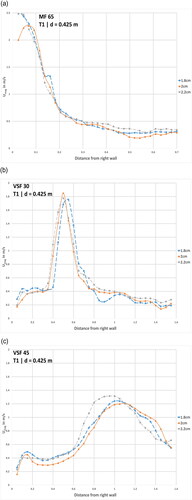
In addition to the GCI-study, we made a comparison diagram of the mean velocity magnitude for each simulated fishway, evaluated transect and water level to visually check the deviation of the results induced by different spatial discretization. In Figure 16 the comparison of the velocities for the IPOS evaluation scope (transect T1 at d = 0.425 m) and a r ≈ 1.11 can be seen, which shows a sufficient convergence in each case at first sight. Additional mean velocity magnitude diagrams for other transects and depths are provided in the appendix files.² This was also done for the case with r = 2.0 for the MF and VSF 45° case, availiable in the appendix files.³

Figure 16. Comparison of the mean velocity magnitude along transect T1 at d = 0.425 m for the grid refinement ratio r ≈ 1.11 in the MF (a), VSF 30° (b)¹ and VSF 45° (c).

One further limitation is the non-dimensional wall spacing y⁺ in the current simulations. This topic is an essential part of a LES/DES model, which must ideally be fulfilled to ensure a correct simulation. The mesh used in this study deviates from the proposed optimum and is one of the factors to look for during the meshing process. While this improvement is feasible, the increased cell amount of smaller size in complex geometric features like e. g. sharp corners, leads to higher demanding mesh qualtity criteria, that must be fulfilled.

Another difficulty of high-resolution numerical models lies in the proper evaluation of the complete data. As our evaluation method concentrated on applying the IPOS-framework on certain transects inside the fishway, a detailed evaluation of the whole 3D numerical data remains a challenge.

Finally, the IPOS-framework and additional literature state further parameters to analyse. For example, the TKE, Reynolds stresses or drag force are often cited as indicators of turbulent intensity inside flows (Wang et al. 2010; Lacey et al. 2012; Silva et al. 2012). While the TKE focusses on the flow fluctuations, the Reynolds stresses and drag force on fish hold strong interest regarding swimming capacity (Verma et al. 2018). These values could provide improved insights into different flow conditions and be compared in a similar manner. As the evaluation method may seem complex and elaborate, future improvements will help us to comprehend the interaction between the fishway’s hydraulic design in comparison to the swimming capacity of fish in all life stages.

7. Conclusion

The investigated fishway designs show distinctive and distinguishable flow regimes, even though the environmental and hydrological boundary conditions are identical. To grasp turbulent flow, the IPOS-framework provides a number of evaluation categories, parameters and methods to quantify those characteristics in laboratory experiments. The implementation of numerical models is reasonable to accomplish and can be expanded by further parameters such as the Q-criterion, which help to gain a deeper comprehension of the flow.

The advantages of a numerical model combined with the IPOS structured evaluation include the comparability with experimental/laboratory research and different constructional design changes. It offers additional insights into the turbulence parameters and has a higher probe density. The quantification and visualisation of high-intensity eddies through numerical simulations are therefore a benefit for further investigations. Another positive effect is that small structural changes can be quickly implemented. Finally, the numerical method could reduce the time and cost of multiple structural evaluations.

One disadvantage of this method is the high computational costs to obtain correct or sufficient flow structures so that they can be compared with experimental/laboratory research. The results are highly dependable on turbulence model and mesh resolution. Even with reduced computation time by using a hybrid turbulence model, a high-performance computer is required to calculate the simulation time until a steady state for the whole fishway is reached, due to the fine mesh requirement in relation to the minimum relevant eddy size. The validation of the chosen mesh size of 2 cm in the simulations with the GCI method is another issue that could not be resolved adequately due to computational restrictions. Instead, we relied on the anticipated minimum eddy diameter of ≈4 cm invoked by the combination of turbulence model, mesh size and numerical accuracy of an eddy, which should be sufficient to capture the smallest fish-relevant eddies. To ensure the accuracy of the numerical model against laboratory ones or field measurements, further research needs to be conducted. Assuming improvements and lower pricing of cloud computing, these negative points could be resolved in the near future.

The different flow patterns and IPOS evaluations in this study affirm that each of the investigated fishways will inflict different effects on the same fish species. The flow regime in each construction differs based on various parameters, requiring improved evaluation methods and the extraction of fish-specific strains swimming inside the flow. This can be achieved by either an experimental “sensor” fish body in laboratory experiments or a “virtual” fish within numerical models. At present, these methods are subject of research at the IWD.

Acknowledgement

We would like to thank the Centre for Information and High Performance Computing (ZIH) at the TU Dresden for the necessary computation resources and support in this project.

Disclosure statement

No potential conflict of interest was reported by the authors.

Notes

1 Appendix files available through following link:https://cloudstore.zih.tu-dresden.de/index.php/s/nxZTaXDYxqSkxiF

2 Direct link to the mean velocity magnitude diagrams (r ≈ 1.11):https://cloudstore.zih.tu-dresden.de/index.php/s/MjkCnbfH972jJ8e

3 Direct link to the mean velocity magnitude diagrams (r ≈ 2.0):https://cloudstore.zih.tu-dresden.de/index.php/s/4AckMAeYT8o4KAM

1 The simulation for a mesh size of 1.8 cm was unstable in terms of residual handling and could only be validated until t = 101.2 s or 30 time steps. The error source could not be found.

References

- ANSYS, Inc. 2014. Introduction to ANSYS Fluent. Turbulence modeling. Limitations of wall-functions. ANSYS, Inc.
- Blevins RD. 1990. Flow induced vibration. 2nd edition, Van Nostrand Reinhold (reprinted by Kreiger, 1993).
- BMUB/UBA. 2016. Water Framework Directive. The status of German waters 2015. Bonn: Umweltbundesamt.
- Bombač M, Četina M, Novak G. 2017. Study on flow characteristics in vertical slot fishways regarding slot layout optimization. Ecol Eng. 107:126–136.
- Cada GF, Odeh M. 2001. Turbulence at hydroelectric power plants and its potential effects on fish. Report to Bonneville Power Administration, United States: N. p., 2001. Web. doi:10.2172/781814.
- Celik IB, Ghia U, Roache PJ, Freitas CJ, Coleman H, Raad PE. 2008. Procedure for estimation and reporting of uncertainty due to discretization in CFD applications. J Fluids Eng. 130(7):78001.
- CFDyna. 2015. A-priori estimation of boundary layer height for mesh generation. Y-plus: estimation of first layer height near wall; [Accessed 2020 Oct 15]. http://www.cfdyna.com/CFDHT/Y_Plus.html.
- Cotel AJ, Webb PW, Tritico H. 2006. Do Brown Trout choose locations with reduced turbulence? Trans Am Fish Soc. 135(3):610–619.
- Duguay JM, Lacey RWJ, Gaucher J. 2017. A case study of a pool and weir fishway modeled with OpenFOAM and FLOW-3D. Ecol Eng. 103:31–42.
- DWA. 2014. Fischaufstiegsanlagen und fischpassierbare Bauwerke. Gestaltung, Bemessung, Qualitätssicherung (DWA-Regelwerk: M, Merkblatt, 509). Hennef: DWA Dt. Vereinigung für Wasserwirtschaft Abwasser und Abfall e.V.
- Enders EC, Boisclair D, Roy AG. 2003. The effect of turbulence on the cost of swimming for juvenile Atlantic salmon (Salmo salar). Can J Fish Aquat Sci. 60(9):1149–1160.
- European Community. 2000. Directive 2000/60/EC of the European Parliament and of the Council of 23 October 2000 establishing a framework for Community action in the field of water policy. Anal Proc. 21(6):196.
- Fehér J, Gáspár J, Veres KS, Kiss A, Globevnik L, Peterlin, M., Kirn, T., Stein, U., Prins, T., Spiteri, C., Laukkonen, E., Heiskanen, A.-S., Austner, K., Semeradova, S., Künitzer, A. 2012. Hydromorpholgical alterations and pressures in European rivers, lakes, transitional and coastal waters. Thematic Assessment for EEA Water. Vol. 2.
- Gerstner CL. 1998. Use of substratum ripples for flow refuging by Atlantic cod. In: Environmental Biology of Fishes. 51 (4)S. :455–460.
- Gisen DC, Weichert RB, Nestler JM. 2017. Optimizing attraction flow for upstream fish passage at a hydropower dam employing 3D Detached-Eddy Simulation. In: Ecol Eng. 100S. :344–353.
- Gramlich M. 2012. Numerical Investigations of the Unsteady Flow in the Stuttgart Swirl Generator with OpenFOAM [Master Thesis]. Gothenburg, Sweden: Chalmers University of Technology. Department of Ap-plied Mechanics, Division of Fluid Dynamics.
- Greenshields CJ. 2015. OpenFOAM programmer's guide. UK: Open-FOAM Foundation Ltd.
- Gritskevich MS, Garbaruk AV, Schütze J, Menter FR. 2012. Development of DDES and IDDES formulations for the k-ω shear stress transport model. Flow Turbulence Combust. 88(3):431–449.
- Höger V, Musall M, Sokoray-Varga B. 2015. Hydraulik von Fischaufstiegsanlagen in Schlitzpassbauweise. physikalische und numerische Untersuchungen zur Optimierung der Passierbarkeit. Germany: Bundesanstalt Für Gewässerkunde.
- Holmén V. Methods for vortex identification. Mathematics (Faculty of Engineering), Master’s Theses. Lund University Libraries.
- Holmén V. 2012. Methods for vortex identification [master thesis]. Lund: Faculty of Engineering, Lund University. https://lup.lub.lu.se/student-papers/search/publication/3241710 (accessed on November 23, 2020).
- Hunt J, Wray A, Moin P. 1988. Eddies, streams, and convergence zones in turbulent flows. In: Studying turbulence using numerical simulation databases. Vol. 1. p. 193–208.
- Jähnel C. 2017. Hydraulische Untersuchungen zur Anströmung von Schlitzöffnungen in Rundbeckenpässen. Study Project. Dresden: Institut für Wasserbau und THM, Technische Universität Dresden.
- Lacey RWJ, Neary VS, Liao JC, Enders EC, Tritico HM. 2012. The IPOS framework: linking fish swimming performance in altered flows from laboratory experiments to rivers. River Res Appl. 28(4):429–443.
- Liao JC, Beal DN, Lauder GV, Triantafyllou MS. 2003. Fish exploiting vortices decrease muscle activity. Science. 302(5650):1566–1569.
- Liao JC. 2007. A review of fish swimming mechanics and behaviour in altered flows. Philos Trans R Soc Lond B Biol Sci. 362(1487):1973–1993.
- Lohnstein J. 2016. Hydraulische Untersuchung der Rund-beckenpassanlage Höxter/Godelheim [diploma thesis]. Dresden: Technische Universität Dresden.
- Musall M, Oberle P, Henning M, Weichert R, Nestmann F. 2014. Analysen zu Strömungsmustern in technischen Fischaufstiegsanlagen. Dresden: Gesellschaft der Förderer des Hubert-Engels Institut.
- Nikora VI, Aberle J, Biggs BJF, Jowett IG, Sykes JRE. 2003. Fish size, time to fatigue, and turbulence on swimming performance: a case study of Galaxias maculatus. J Fish Biol. 63(6):1365–1382.
- Pavlov DS, Lupandin AI, Skorobogatov MA. 2000. The effects of flow turbulence on the behaviour and distribution of fish. J Ichthyol. 40:232–261.
- Peters HW. 2004. Der Mäander Fischpass. Wasserwirtsch. 94(7–8):33–39.
- Rajaratnam N, van der Vinne G, Katopodis C. 1986. Hydraulics of vertical slot fishways. J Hydraul Eng. 112(10):909–927.
- Rajaratnam N, Katopodis C, Solanki S. 1992. New designs of vertical slot fishways. Canadian J. Civil Engineering, 19(3):402–414
- Rodi W. 2017. Turbulence modeling and simulation in hydraulics: a historical review. J Hydraul Eng. 143(5):03117001.
- Roth MS. 2019. Implementierung einer geometrischen Rauheit für Wandrandbedingungen in der 3D-HN-Modellierung [Implementation of a geometric roughness for wall-boundary-conditions in 3D-CFD-models] [diploma thesis]. Dresden: Technische Universität Dresden, Institut für Wasserbau und Technische Hydromechanik.
- Schlichting H, Gersten K. 2017. Boundary-layer theory. Unter Mitarbeit von Egon Krause und Herbert Oertel. 9th ed. Berlin (Heidelberg): Springer.
- Schneider LK. 2017. Hydro-numerical investigations concerning the influence of two different turbulence modeling approaches (RANS with k-e-equation and LES) within two types of fish migration facilities (Vertical Slot Fish Pass and Meander-Type Fish Pass) [master’s thesis]. Dresden: Technische Universität Dresden.
- Schulze L, Thorenz C. 2014. The multiphase capabilities of the CFD toolbox OpenFOAM for hydraulic engineering applications. Hg. v. International Conference on Hydro-Science and -Engineering; Hamburg.
- Silva AT, Katopodis C, Santos JM, Ferreira MT, Pinheiro AN. 2012. Cyprinid swimming behaviour in response to turbulent flow. Ecol. Eng., 44:314–328 doi:10.1016/j.ecoleng.2012.04.015
- Slater JW. 2008. Examining spatial (grid) convergence. NPARC Alliance CFD Verification and Validation Web Site; [Accessed 2008 Jul 17] https://www.grc.nasa.gov/www/wind/valid/tutorial/spatconv.html.
- Spalart PR. 2001. Young-Person's guide to detached-eddy simulation grids. Unter Mitarbeit von Craig Streett. Seattle (WA): NASA, Boeing Commercial Airplane Group. [Accessed 2020 Jun 17]. https://ntrs.nasa.gov/search.jsp?R=20010080473.
- Spalart PR. 2009. Detached-Eddy simulation. Annu Rev Fluid Mech. 41(1):181–202.
- Stamm J, Helbig U, Seidel C, Zimmermann R, Martin H. 2015a. Hydraulische Charakteristik von Rundbeckenpässen (45). Proceedings in Internationales Wasserbau-Symposium Aachen.
- Stamm J, Helbig U, Zimmermann R. 2015b. Hydraulic characteristics of meander-type fish passes. Proceedings of the 36th IAHR World Congress, 2015, Deltas of the Future and What Happens Upstream Proceedings held between 28 June - 3 July 2015, The Hague, The Netherlands.
- Tallin University of Technology. 2018. Differential pressure sensor base artificial lateral line probe, iRon. Estonia: Centre for Biorobotics, Tallin University of Technology (TUT), FIThydro; [Accessed 2020 Sep 30]. https://www.fithydro.wiki/index.php/Differential_pressure_sensor_base_artificial_lateral_line_probe.
- Tritico HM, Cotel AJ. 2010. The effects of turbulent eddies on the stability and critical swimming speed of creek chub (Semotilus atromaculatus). J Exp Biol. 213(Pt 13):2284–2293.
- Tudorache C, Viaene P, Blust R, Vereecken H, Boeck GD. 2008. A comparison of swimming capacity and energy use in seven European freshwater fish species. Ecol Freshwater Fish. 17(2):284–291.
- Verma S, Novati G, Koumoutsakos P. 2018. Efficient collective swimming by harnessing vortices through deep reinforcement learning. Proc Natl Acad Sci U S A. 115(23):5849–5854.
- Wang RW, David L, Larinier M. 2010. Contribution of experimental fluid mechanics to the design of vertical slot fish passes. Knowl Manag Aquatic Ecosyst. 396(396):02.
- Webb PW. 1998. Entrainment by river chub nocomis micropogon and smallmouth bass micropterus dolomieu on cylinders. J Exp Biol. 201(Pt 16):2403–2412.
- Wilcox DC. 2010. Turbulence modeling for CFD. 3rd ed. La Cañada (CA): DCW Industries.
- Williamson CHK. 1996. Vortex dynamics in the cylinder wake. Rev Fluid Mech. 28:477–539.
- Wu S, Rajaratnam N, Katopodis C. 1999. Structure of flow in vertical slot fishway. J Hydraul Eng. 125(4):351–360.