Computational fluid dynamics simulation of passive downstream fish passage over a weir with OpenFOAM^®

Abstract

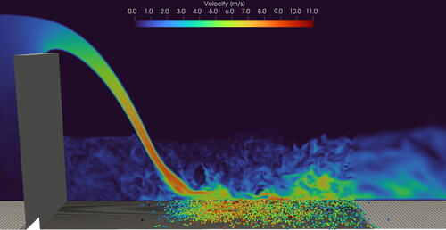
Many fish species are dependent on migration through river systems. Weirs are an obstacle to downstream migration, which can lead to obstruction as well as injury and mortality. The current level of knowledge about downstream migration over weirs is limited, and the current assessment of this is uncertain. This study uses a computational fluid dynamics (CFD) method for assessing the damage potential of the downstream migration over the weir, evaluating the effectiveness of the current recommendations. Two test cases were simulated using OpenFOAM^® and an interFoam-based solver, extended with Lagrangian particles to represent passively transported fish. The results of the simulations show that adherence to the recommendation for a necessary tailwater level has no significant impact on the relevant hydraulic stressors, shear stress, pressure changes and collisions in certain situations. A thick nappe, however, leads to a significant reduction in collisions, especially of particles initialized near the surface. The CFD method used in this study proves to be suitable for evaluating downstream fish passage with certain limitations. This means that qualitative comparisons of different situations are possible, but not the determination of the damage potential of a specific situation. Further investigations are necessary to identify factors for safe downstream fish passage.

Keywords:

• Downstream fish passage
• weir
• CFD
• particle simulation
• OpenFOAM

1. Introduction

For both navigation and renewable energy production, there are many weirs on German waterways and around the world. However, there are also adverse effects of weir structures on the environment, including the river continuity (Belletti et al. 2020). As a result, weirs affect fish populations, especially diadromous species that migrate between freshwater and marine habitats to reproduce (Watson et al. 2018), but also potamodromous species moving within freshwater (Barbarossa et al. 2020), contributing to declining fish stocks worldwide (Pelicice et al. 2015; Schilt 2007; Silva et al. 2018). While obstruction is the main problem for upstream migrating fish, the downstream passage can result in fish injury or mortality in addition to obstruction (Scruton et al. 2008).

Weir structures, especially those including hydropower plants, typically have several possible routes for fish to pass. These pose varying risks to fish (Schwevers and Adam 2020). Passage through turbines is usually associated with high risk and has been frequently investigated (Čada 2001; Deng et al. 2011; Eyler et al. 2016; Skalski et al. 2002). However, passage above or below the weir can also be associated with risks of injury or mortality. Here, the current level of knowledge is still relatively low compared to turbine passage (Pflugrath et al. 2019). Typical causes of injury include pressure changes, especially in undershot weirs, collisions with parts of the weir structure, the plunge pool floor or installations in the downstream area, as well as high shear whenever water masses with different velocity trajectories meet or near the weir crest and the channel bottom (Baumgartner et al. 2014).

It is important to improve the design and operation of the hydropower unit to reduce ecological impact. However, the passage over the weir itself must also be designed as safely as possible for fish. In Germany, the evaluation of weir passage is currently carried out using the recommendation of the German Association for Water, Wastewater and Waste (DWA 2021). The DWA recommends a water depth below the impoundment of more than one-quarter of the water level difference but at least 0.9 m. Furthermore, the plunge pool is recommended to have a volume of at least 10 m³ per 1 m³/s flow to avoid high shear forces (DWA 2021) as recommended by Odeh and Orvis (1998). It should be noted that there is no reference to experiments conducted by Odeh and Orvis regarding fish damage, and no background is given for the values mentioned, except that they are the basic design characteristics of downstream fish passage facilities used in 1998 by the US Fish and Wildlife Service. It should also be considered that the recommendations regarding tailwater depth by Odeh and Orvis (1998) were intended for bypass systems and may not necessarily be a useful application for the weir itself. The situation at the weir differs significantly from that of a bypass system, particularly with regard to flow and water propagation direction. Typically, the water jet of a bypass system leads into a plunge pool that remains almost unaffected by the slight water and energy input from the bypass system, and the water can spread in all directions. In contrast, the flow over the weir is usually much larger, and the nappe can only spread in the direction of the tailwater. This leads to a significant influence on the situation in the plunge pool. The hydraulic jump can be shifted into the tailwater by the nappe, resulting in supercritical flow at the point of impact and, therefore, a lack of necessary water cushion, even if the required tailwater depth is present downstream. This raises questions as to whether applying the tailwater criterion is also feasible for the weir overflow (Thorenz et al. 2018).

Recent field trials have raised additional concerns as to whether the tailwater criterion is able to avert injury to fish. Knott et al. (2022) observed fish mortality and Pflugrath et al. (2019) potentially harmful collisions with the plunge pool floor in situations adhering to the recommendations by the DWA. However, due to a small sample size and low water level difference, respectively, these studies are only of limited comparability. Based on these observations, Mueller et al. (2022) suggest increasing the required plunge pool depth to 70% of the water level difference, whereas Pflugrath et al. (2019) call for further testing at overshot weirs with varying plunge pool depths.

However, in addition to whether the tailwater criterion of at least a quarter of the water level difference is sufficient, there is a fundamental question of whether an increase is advisable or whether this criterion needs to be fundamentally reconsidered. A theoretical water cushion, regardless of its height, does not fulfil its function if it is displaced into the tailwater due to the hydraulic situation caused by the weir overflow. Thorenz et al. (2018) examined the applicability of the tailwater criterion for the weir overflow using numerical simulations. Two stylized weirs, each with situations where the tailwater criterion is not met and situations where the tailwater criterion is met, were simulated. In these situations, at least visually, the difference between the situations adhering to the criteria and those not adhering to it is marginal. Of greater importance seems to be the nappe thickness and the angle of impact of the nappe on the plunge pool floor.

In summary, there are strong doubts about the tailwater criterion’s efficacy. However, due to the lack of alternatives, it is still applied. In addition to the tailwater criterion, the DWA (2005) recommends a maximum impact velocity on water of 13 m/s. This value is based on a series of tests conducted between 1939 and 1972 with fish of various sizes, summarized by Bell and DeLacy (1972) and later by the US Army Corps of Engineers (USACE 1991). Based on these publications, Ebel (2013) identifies a critical value of 16 m/s for the onset of injury to gills, eyes and internal organs in fish but also recommends a value of 7–8 m/s to prevent injuries reliably. The basis for these are recommendations for bypass systems by the National Marine Fisheries Service (NMFS 1995, 1997) and the Washington Department for Fish and Wildlife (WDFW 2000). These publications do not cite any research that led to the mentioned values. More recent experiments regarding the impact velocity are not available. One issue not addressed by the DWA (2005) is rapid pressure changes, despite being a major factor for injury, particularly at undershot weirs (Pflugrath et al. 2019). Generally, all cited recommendations and criteria are based on a minimal number of actual trials, some of which are not documented and traceable.

Downstream fish passage over weir structures is an issue that needs to be addressed to improve the knowledge of acceptable and unacceptable conditions. A common method of evaluating the hazard potential for fish in existing structures is a live fish field study. These have been carried out extensively on Kaplan turbines (Dauble et al. 2007; Hughes et al. 2013; Trumbo et al. 2014) but also on Francis turbines (Dedual 2007), Archimedes screws (Pauwels et al. 2020) and in a limited number on weirs themselves (Baumgartner et al. 2006; Duncan 2013; Knott et al. 2022). The physical conditions during downstream passage can also be directly measured using passive sensors (Deng et al. 2014; Fu et al. 2016; Pauwels et al. 2022). The main disadvantage of these methods is that they can only be applied to existing structures. In addition, the expense for such studies is immense, the sample size accordingly often limited, and the assessment of the cause and location of injury difficult. One way to evaluate a weir during the design phase is through physical models. These offer the possibility to analyse and evaluate the hydraulic situation. On the other hand, due to scale effects, it is usually not possible to monitor the actual hazard potential with live fish since the body size of live fish cannot be adapted to scale (Adam and Lehmann 2011). An exception to this is ethohydraulic models. The disadvantage is the enormous additional effort due to the necessary size of the model as well as the fish handling. Generally, methods that do not harm live creatures are preferable.

An alternative approach for the investigation of the hazard potential of the weir passage is computational fluid dynamics (CFD), using particles to simulate fish. Various approaches are being pursued to model fish passage with CFD. Zhu et al. (2022) evaluated quantitatively the pressure and shear damage probability for a Francis turbine using CFD simulation. Romero-Gomez and Richmond (2017) used CFD models to simulate the movement and collisions of Lagrangian particles in hydro-turbine intakes and validated the simulations using a laboratory physical model and an autonomous sensor device. The accuracy of simulating Lagrangian neutrally buoyant inertial spheres moving in subcritical flow was verified using experimental data in a laboratory flume (Romero-Gomez et al. 2022). Another method based on Lagrangian particles to predict the relative risk of injury and mortality for fish during turbine passage was further validated by comparison to analytical values for moving particles and physical experimental data for trajectories and collisions of particles (Singh et al. 2021). Richmond et al. (2014) evaluated blade strike and rapid pressure change during the turbine passage using streamtracers to estimate a fish’s path and the discrete element method (DEM) to model fish-like composite particles. The resulting measurements were compared to previous field studies with passive sensors. DEM was used as well by Singh et al. (2022) to detect the hazard potential of fish passage through a Kaplan turbine due to pressure change, shear and collision. Benigni et al. (2021, 2022) simulated downstream fish migration through Kaplan turbines, focusing on the differences between steady-state and transient CFD calculations.

Overall, our understanding of downstream fish migration below or above weirs is still unsatisfactory and mainly limited to individual facilities. Studies with live fish or passive sensors can only be applied to existing structures and physical models are not applicable to the large variety of different system types and situations. For these reasons, CFD simulations were chosen to address the issue despite limitations stemming from the simplified depiction of the fish. The objective of this work is to draw up a method to describe the situation of downstream fish migration over or under weirs and its physical effects on fish. This article describes a study based on CFD simulations with Lagrangian particles using the open-source simulation package OpenFOAM^® to evaluate downstream fish passage. First, an overview of the modelling approach, using unsteady, large eddy simulation (LES) to resolve velocity fluctuations, is provided. This approach is then used to further evaluate the recommendation for the plunge pool depth by the DWA (2005) and to test the practical application on an actual weir. The results of these simulations are presented. Finally, the usability of the described modelling approach and its limitations are discussed and summarized.

2. Method description

2.1. Computational fluid dynamics

2.1.1. OpenFOAM

To simulate the passive downstream passage of fish over a weir, the open-source CFD library OpenFOAM^® was used. OpenFOAM^® uses the finite volume method to solve partial differential equations and provides a wide range of solvers, each tailored to model specific physical phenomena. For this study, an adapted solver based on the two-phase solver interFoam from OpenFOAM^® version 2012 (Bracknell, UK) extended with Lagrangian particles was used. The solver interFoam is based on the volume of fluid method (Hirt and Nichols 1981) for simulating two-phase flows with an interface between two immiscible fluids, for which the Navier Stokes equations are solved (Deshpande et al. 2013; Rusche 2003). It is widely used to simulate free-surface flows (Gisen et al. 2017; Thorenz and Schulze 2021). The implemented equations for mass and momentum are formulated as follows: (1) $$\nabla \bullet \mathit{\text{U}}=0$$(1) (2) $$\frac{\partial \rho U}{\partial t}+\nabla \bullet \left(\rho \mathit{\text{UU}}\right)=-\nabla p_{\mathit{\text{rgh}}}+\nabla \bullet \mu \left(\nabla U+{\nabla U}^T\right)+\rho g+F$$(2) where U is the velocity vector, ρ is the density of the mixture of the two phases, t is time, p_rgh is a modified pressure that is used instead of p, and µ is the dynamic viscosity of the fluid mixture. The following equation shows the relationship of p_rgh and p: (3) $$p_{\mathit{\text{rgh}}}=p-\rho g\bullet h$$(3)

F is a continuum surface tension force model described by Brackbill et al. (1992), but which is of little importance in the cases considered. With this formulation of the continuity equation, it is assumed that the fluid is incompressible and has a constant density. In addition, interFoam solves a scalar transport equation to model the movement of the distribution of air and water: (4) $$\frac{\partial \alpha }{\partial t}+\nabla \bullet \left(\alpha U\right)+\nabla \bullet \left[\right(1-\alpha \left)\alpha U_c\right]=0$$(4) where α is the volume fraction of the total volume that is occupied by water, with 0 ≤ α ≤ 1. U_c is an artificial compression velocity implemented in the interFoam solver to avoid the smearing of the interface between the two phases when solving the phase fraction equation (Equation (4)(4) $$\frac{\partial \alpha }{\partial t}+\nabla \bullet \left(\alpha U\right)+\nabla \bullet \left[\right(1-\alpha \left)\alpha U_c\right]=0$$(4) ) with the finite volume method (Okagaki et al. 2021; Peltonen et al. 2020). The introduction of α results in the following equations for the dynamic viscosity µ and the density ρ of the fluid mixture: (5) $$\mu =\alpha \bullet {\mu }_1+\left(1-\alpha \right)\bullet {\mu }_2$$(5) (6) $$\rho =\alpha \bullet {\rho }_1+\left(1-\alpha \right)\bullet {\rho }_2$$(6)

2.1.2. Turbulence modelling

Turbulence is an essential and omnipresent feature of many fluid flows, and its adequate prediction is critical for a wide range of applications. Because turbulence is a highly nonlinear and seemingly chaotic phenomenon that involves a wide range of spatial and temporal scales, turbulence modelling is one of the most challenging aspects of CFD. Today, Reynolds-averaged Navier–Stokes (RANS) is still the most common turbulence modelling method used in industrial and research applications due to its computational efficiency and stability (Yusuf et al. 2020; Zhao et al. 2020). In RANS, turbulent fluctuations are modelled as a time-averaged component, which has limitations in capturing unsteady and large-scale turbulent structures. This is especially inconvenient when modelling a particle’s path. A time-averaged flow field tends to evade obstacles, which would lead to an underestimation of collisions. To avoid a time-averaged flow field and directly simulate all eddies which could alter the particle’s path, direct numerical simulation (DES) would be necessary, which is practically not possible. Therefore, LES was chosen to at least simulate all highly energetic larger eddies. LES resolves the largest turbulence structures directly while the smaller, less energetic eddies are modelled using sub-grid scale models, which makes it more accurate in predicting turbulent variation than RANS but computationally more expensive (Rodi 2017). A wide variety of different subgrid models for LES is available in OpenFOAM^®. In this study, the commonly used turbulence model k-equation was used (Yoshizawa 1986).

2.1.3. Lagrangian particles

There is a wide range of available solvers for different kinds of particle-laden flow in OpenFOAM^®. Prominent examples are DPMFoam, which is a highly customizable solver using the Discrete Phase Model, a Lagrangian approach for modelling the behaviour of particles in a fluid (Fernandes et al. 2018), or MPPICFoam, which uses the Lagrangian Multi-Phase Particle In Cell method to simulate the behaviour of multiphase flows, particularly the behaviour of particles suspended in a fluid (Andrews and O’Rourke 1996). While these solvers have been proven to work as intended in many cases, they include a multitude of sophisticated models to depict processes like heat transfer or particle-particle interactions that are not necessary for this study but increase the complexity. Furthermore, to simulate the weir passage, a multiphase solver is necessary. For these reasons, the two-phase solver interFoam was extended with the basicKinematicCloud, a simple Lagrangian particle phase.

The basicKinematicCloud is designed to be flexible and adaptable. It provides a framework for implementing various kinematic models for particle motion. Generally, the basic motion for a particle, based on Newton’s second law of motion, can be written as follows: (7) $$m\frac{\mathit{\text{du}}}{\mathit{\text{dt}}}=\sum F_i=F_D+F_G+F_P+F_{\mathit{\text{VM}}}+F$$(7) where m is the mass of the particle, u is its velocity, and ∑F_i is the sum of all forces on the particle. F_D is the drag force, F_G is the gravitational force, F_P is the force due to a local pressure gradient, F_VM is the virtual mass or added mass force, and F stands for all other but less prominent forces like rotational or shear lift forces and thermophoretic forces. Because the density of the used particles is equal to the water’s density and, therefore, the gravitational and buoyancy forces cancel each other out, the predominant forces in the fluid-particle flow are the drag force F_D and the virtual mass force F_VM. The general formulation for F_D expressed in terms of the drag coefficient C_D is: (8) $$F_D=C_D{A}_p{\rho }_f(u_f-u_p)\left|u_f-u_p\right|$$(8) where A_P is the projected area of the particle, ρ_f is the fluid density, u_f is the fluid velocity and u_p the particle velocity. The implemented model for the drag coefficient C_D is the drag correlation by Putnam (1961), which is applicable to spherical solid particles. The equation is written as shown below: (9) $$C_D=\{\begin{array}{l}\frac{24}{{\mathit{\text{Re}}}_p}\left(1+\frac{1}{6}{\mathit{\text{Re}}}_p^{2/3}\right)\mathit{\text{if }}{\mathit{\text{Re}}}_p\le 1000\\ 0.44\mathit{\text{ if }}{\mathit{\text{Re}}}_p>1000 \end{array}$$(9) where Re_p is the particle Reynolds number, which is defined as follows: (10) $${\mathit{\text{Re}}}_p=\frac{{\rho }_f\bullet u_p\bullet d_p}{{\mu }_f}$$(10) where d_p is the characteristic diameter of the particle, and µ_f is the dynamic viscosity of the fluid. For higher particle volume fractions, various drag models exist but have not found application due to the low volume fraction used. The equation for F_VM is formulated as follows: (11) $$F_{\mathit{\text{VM}}}=V_p{\rho }_f(\frac{D{u}_f}{\mathit{\text{Dt}}}-\frac{d{\mathit{u}}_{\mathit{p}}}{\mathit{\text{dt}}})$$(11) where V_p is the volume of the particle, and D/Dt denotes the material derivative. Besides the drag force F_D, the following forces are included in the used model: the gravitational force F_G, the lift force F_L, the virtual mass force F_VM and F_P and the force due to a local pressure gradient.

Apart from the particle movement due to the flow of the carrier fluid that each particle modelling method integrates, feedback on the fluid or particle-particle interaction is only present in higher orders of coupling. The necessary order of coupling between the particle and the fluid is typically determined by the volume fraction of the particle phase α_p = V_P/V_F. According to Elghobashi (1994) in flows with α_p ≤ 10⁻⁶, the particles have a negligible effect on the carrier fluid, so one-way coupling is sufficient. A volume fraction of α_p ≤ 10⁻³ requires additional particle-particle interaction, i.e. four-way coupling. Although a particle volume fraction of this order may occur, one-way coupling was chosen. The reason for this is that each particle moves independently of one another. This leads to the advantage that virtual volume fractions (unnatural number of particles per volume) can be realized in a single simulation without mutual influence: Instead of many simulations with a single or only a few particles, one simulation with many particles is sufficient.

In addition to the particle basic movement, the used method includes a model for the interaction with each patch of the computational domain. Particles can either escape through a patch, stick to it or rebound. An elasticity and a restitution coefficient describe the rebound velocity. The strictly spherical particles themselves are described by a diameter and a density. They do not have any other properties. A wide variety of injection models to initialize the particles is available. For this study, only the manualInjection was used, where the starting position of each particle is defined in a position file.

2.1.4. Particle injection position

Because the forces acting on a fish during the weir passage are also dependent on the passage corridor, the injection position of the particles is of great importance. A statistical analysis assumes a uniformly distributed sample. Since fish do not migrate uniformly distributed over the whole cross-section, but the actual migration corridors depend on the species and other factors (Knott et al. 2023; Larinier and Travade 2002), the cross-section flowed through above the weir crest is divided into individual starting windows. These should be, with regard to the hydraulic conditions, as homogeneous as possible within themselves and different from the other starting windows. The statistical analysis can thus be carried out individually for the homogeneous starting windows, and an equally distributed population can be assumed. To achieve temporal variance, these starting windows are extended upstream along the streamlines, creating 3D areas in which the particles are initialized. These cover a space with a flow velocity of about 1–3 m/s, roughly the range of the usual maximum swimming speed of European freshwater fish (Ebel 2014). The spatial distribution creates temporal variance. To achieve a confidence level of 95% and a margin of error of 2%, a sample size of 2401 particles is initialized randomly in each area for each simulation (Israel 1992).

After injection, the particle’s position, velocity and the hydraulic situation surrounding the particle are tracked discretely. For this study, a tracking interval of 0.01 s was chosen. The amount of data generated and the corresponding storage space required depends on the tracking interval. Postprocessing also becomes costlier with the number of data points. Significantly smaller tracking intervals are therefore impractical. The selected interval represents a good compromise between effort and accuracy and also enables simple conversions. The simulation duration depends on the specific case; the particles should have passed through the area associated with high. This was the case after 5 s for the simplified overhot weir and after 10 s for Pulverweiden weir.

2.1.5. Particle postprocessing

The necessary data for the particle processing is recorded during the simulations. These are the cell values pressure (p), velocity (U), velocity gradient (gradU), phase distribution (alpha.water) and once the wall distance (wallDistance) as well as the particle values position (positions), identification number (origId) and particle velocity (U). The postprocessing was done using Python version 3.10.9 (Wilmington, DE, USA). Figure 1 shows a flowchart of the data processing done.

Figure 1. Flowchart of the data processing done. The values are output for each time step and particle.

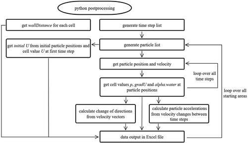
The output per tracking interval and particle is then used to determine the maximum values for pressure fluctuation, shear stress and collision as well as the corresponding velocity and impact angle. The precise calculation of these values is described in the following chapters.

2.2. Hydraulic stressors

During the passage across hydraulic structures, fish are exposed to a variety of influences that can lead to injury or even mortality. The typical hydraulic stressors that are reported in the literature are shear stress, pressure changes, acceleration, turbulence, gas supersaturation, physical strike and collision (Cox et al. 2023). Due to the limited weir heights, especially collisions, but also shear stress and pressure changes are considered particularly relevant for German waterways (Kaminski et al. 2021; Schmalz et al. 2015). Whereas strike is mainly associated with turbine passage and is not considered at weirs due to the lack of moving parts, acceleration, turbulence and aeration theoretically also cause injury at weir structures. Due to the modest height differences of German weirs, gas supersaturation in particular, but also acceleration, is of less importance (Mao et al. 2022; Nielsen and Szabo-Meszaros 2022). While turbulence is usually not harmful in itself, it can lead to disorientation and, therefore, increased predation (Čada 2001). Since predation is not directly depictable in the numerical simulations, turbulence was not analysed.

2.2.1. Shear stress

Shear stress is a commonly identified hydraulic stressor and is relevant for both undershot and overshot weirs (Baumgartner et al. 2017; Čada et al. 1999; Neitzel et al. 2000). Areas where potentially lethal levels of shear stress occur are wherever two bodies of water moving at different velocities meet (Čada 2007). Typical injuries due to shear stress include decapitation, descaling, eye loss, fin, operculum or gill damage, haemorrhaging and spinal injury (Cox et al. 2023). Because shear is a naturally occurring phenomenon, some species are better adapted and have higher tolerances to shear stress than others. The majority of studies have analysed the impact of high shear stress on North American species (Čada et al. 1999; Čada and Charles 1997; Čada 1990; Deng et al. 2005, 2010; Killgore et al. 2001; Neitzel et al. 2000, 2004; Odeh et al. 2002; Turnpenny et al. 1992) while more recently some studies also focused on Australian species (Boys et al. 2014; Navarro et al. 2019) and Southeast Asian species (Baumgartner et al. 2017; Colotelo et al. 2018; Thorncraft et al. 2013).

For a parallel flow of a Newtonian fluid, shear stress τ can be described by the following equation: (12) $$\tau =\mu \frac{\partial u}{\partial y}$$(12)

where µ is the dynamic viscosity and ∂u/∂y is the velocity gradient perpendicular to the flow direction. Also commonly used, especially in laboratory experiments, is the time-averaged strain rate e, the average velocity difference $d\overline{u}$ divided by the distance dy, which is often defined as the width of the fish (Neitzel et al. 2004). The consideration of different values of dy makes quantitative comparison between reported results problematic (Cox et al. 2023). In this study, shear stress τ [mPa] is used. Since the dynamic viscosity µ of water at 20 °C is 1.0 [mPa*s], the values for the shear stress τ [mPa] are equivalent to those of the strain rate e [m/(m*s) or s⁻¹] assuming a complete filling with water of 20 °C. In OpenFOAM^®, shear stress τ is accessible through the velocity gradient gradU, which is calculated for each cell as the velocity change in all three directions between the cell centre and the respective cell face over the respective distance. The distance depends on the computational grid discretization. The velocity gradient from the centre of the cell to the surrounding cell faces is calculated. Accordingly, a velocity gradient tensor is produced, which looks as follows: (13) $$\mathit{\text{gradU}}=\begin{array}{ccc}\frac{\mathit{\text{dU}}\_x}{\mathit{\text{dx}}}& \frac{\mathit{\text{dU}}\_x}{\mathit{\text{dy}}}& \frac{\mathit{\text{dU}}\_x}{\mathit{\text{dz}}}\\ \frac{\mathit{\text{dU}}\_y}{\mathit{\text{dx}}}& \frac{\mathit{\text{dU}}\_y}{\mathit{\text{dy}}}& \frac{\mathit{\text{dU}}\_y}{\mathit{\text{dz}}}\\ \frac{\mathit{\text{dU}}\_z}{\mathit{\text{dx}}}& \frac{\mathit{\text{dU}}\_z}{\mathit{\text{dy}}}& \frac{\mathit{\text{dU}}\_z}{\mathit{\text{dz}}}\end{array}$$(13)

where dU_x, dU_y and dU_z are the velocity changes in x-, y- and z-direction, respectively and dx, dy and dz are the distances in the respective direction. These changes in velocity are caused by rotation, the antisymmetric part of the gradU tensor, and strain, the symmetric part. On the considered size scale of the cell, it can be assumed that the effect on fish of the velocity gradient is the same regardless of its origin. Accordingly, no separation is undertaken, but rather, the absolutely highest value outside the main diagonal of these nine is used approximately as the strain rate e. The main diagonal is ignored because these velocity changes cannot lead to shear stress but only compression or stretching. Additionally, this approach is dependent on the coordinate system. The maximum value can be up to $\sqrt{2}$ times higher than the value recorded. Also, as LES turbulence modelling is used, small eddies are not resolved directly but modelled as a time-averaged component. Therefore, this less energetic small-scale part of the turbulent shear stress remains unaccounted for. To summarize this approach does not specify an exact value but only an approximation for the shear stress. The maximum recorded shear stress on the individual particles during the entire weir passage was evaluated.

2.2.2. Pressure changes

Sudden widening or narrowing of the flow cross-section and, thus, the flow velocity or the abrupt change in the water level is caused for rapid pressure changes. Especially quick pressure drops, happening in seconds or less, are known to harm fish (Cox et al. 2023; Pflugrath et al. 2019). Even though minor pressure changes also occur at overshot weirs, they are mainly associated with undershot weirs. The high pressure due to the water depth in front of the weir drops abruptly as the water passes through the weir. Pressure change can lead to injuries like embolism, eye loss, haemorrhaging, operculum damage or swim bladder rupture, which are often irreversible and lethal (Cox et al. 2023). Especially at undershot weirs, rapid pressure change can be the main reason for damage to fish. Consequently, different studies have analysed the impact on North American species (Abernethy et al. 2001, 2002; Brown et al. 2012; Carlson et al. 2010; Doyle et al. 2020; Feathers and Knable 1983; Foye and Scott 1965; Harvey 1963), Australian species (Boys et al. 2014, 2016a, 2016b) and Eurasian species (Doyle et al. 2022; Tsvetkov et al. 1972). Interspecific differences regarding tolerable pressure change levels are mainly due to different types of swim bladders. Whereas physostomes have a pneumatic duct that connects the swim bladder to their intestines, allowing them to expel gas quickly, physoclisti do not have this connection. They can only regulate buoyance slowly by gas diffusion into and out of the swim bladder (Brown et al. 2014). In consequence, physoclisti are likely to be more susceptible to pressure changes.

Pressure changes are usually described using the ratio of pressure change (RPC). RPC is defined as the ratio of exposure pressure P_e to acclimatization pressure P_a: (14) $$\mathit{\text{RPC}}=\frac{P_e}{P_a}$$(14)

P_a is the pressure that a fish is acclimated to and would naturally experience at a certain water depth and P_e is the minimum or maximum pressure the fish experienced during its downstream passage. In this study, Pa is defined as the hydrostatic pressure at the point of initialization. Up to this point, it is assumed that the fish was able to move freely and, hence, acclimate to the situation. Pe is defined as the minimum static pressure. The static pressure in each cell the particle is located in is discretely tracked during the simulation, and the RPC is calculated for each particle.

2.2.3. Collision

As there are no moving parts, only the collision with the weir structure is a factor in the weir passage and not the strike of turbine blades as in a turbine passage. Collisions occur at overshot and undershot weirs. Typical situations are the direct impact of fish on baffle blocks in the stilling basin or the plunge pool floor. At low-head weirs, where height and pressure differences are too small for dangerously high shear stress or pressure changes, collisions can still lead to significant harm to fish (Pflugrath et al. 2019). Collision can usually lead to bruising, descaling, epithelium or eye loss, fin, operculum or gill damage, haemorrhaging and spinal injury. Despite the high importance, the empirical data on collisions is very limited. Based on different field tests, the USACE (1991) created a correlation between fish kill rate and collision velocity.

The applied numerical method has the option of recording collisions of particles with walls. However, because collisions are only detected when the centre of the particle touches the wall, this was not used. When conducting field trials, the detection of collision or strike with passive sensors is often done by evaluating the acceleration peak duration where acceleration values are within 70% of the peak value. Here, it was defined that if the peak duration is less than 0.0075 s, it is considered a collision event (Boys et al. 2013). Since this requires tracking intervall of less than 0.001 s but an intervallof 0.01 s was used, another method was chosen: Accelerations by more than 10 g, based on a change in time of 0.01 s, are counted as collisions if the particle is in a cell less than 0.04 m to the nearest wall. Evaluated is the impact velocity, calculated as the maximum velocity in the two previous time steps. If multiple collisions occur, only the most intense is considered. Additionally, the angle of impact is approximated by determining the trajectories before and after the impact and considering the law of reflection.

3. Case study: simplified overshot weir

As a first test case, a highly simplified rectangular overshot weir erected on a flat surface, based on the numerical study of Thorenz et al. (2018), was chosen. Whereas Thorenz et al. (2018) simulated the hydraulic situation without particles representing fish and evaluated the result visually based on the streamlines, this study utilizes the described method to investigate fish passage over the simplified weir. In this way, this case study aims to either strengthen or weaken the criticism of the tailwater criterion (DWA 2005).

3.1. Model description

In the numerical model, an area with a length of 99.92 m, a width of 2.24 m and a height of 8 m was considered. The rectangular weir was located in the centre, so the lengths of the headwater and tailwater were 50 m and 49.6 m respectively. The computational grid consists of about 18 million hexahedron-dominant cells with a base length of 32 cm. It was iteratively refined in the vicinity of all walls, the nappe and the area of possible particle movement to a cell length of 2.0 cm. The remaining water-filled area was refined to a cell length of 8.0 cm. Since particles cannot be larger than the cells, and to avoid the influence of differing cell sizes on the interpretation of collisions and shear stress, no wall layers were added. A mesh independence analysis was performed with five different mesh refinements with cell lengths of 16.0, 8.0, 4.0, 2.0 and 1.0 cm in the areas of high flow gradients and possible particle movement. The performance of the overflow was tested, i.e. the water level and flow rate as well as the simulated turbulence share as an LES quality criterion. Due to the boundary condition, the headwater level was kept stable in all cases. Differences were less than 1.0 cm. The flow rate averaged over 30 s relative to the case with a cell length of 1.0 cm was 100.8% (cell length 2.0 cm), 101.72% (4.0 cm), 112.58% (8.0 cm) and 107.00% (16.0 cm). Figure 2 shows the highly turbulent area below the weir body of the case with a cell length of 2.0 cm. In the red areas, at least 80% of the turbulent kinetic energy is simulated and less than 20% is modelled by sub-grid models. This is not the case in the blue areas. Except for the low-turbulence nappe itself, this criterion for good LES is fulfilled. As the added particles have to be smaller than the cells to avoid unphysical behaviour, the coarsest grid was selected, which represents the hydraulic situation sufficiently well.

Figure 2. Section of the calculation area with a cell length of 2.0 cm. In red: Areas in which at least 80 % of the turbulent kinetic energy is simulated and less than 20 % is modelled by Sub-grid models. In blue: Areas in which more than 20 % is modelled. The white lines represent the water surface.

Four situations were examined, corresponding to the study by Thorenz et al. (2018). A headwater level of 5 m was fixed by defining the pressure field and the air-water distribution at the inlet patch (Thorenz 2024), whereas the tailwater level, which was set in the same way, varied. For two weir heights of 3 m (W3) and 4 m (W4), two tailwater situations were examined. In one case, the tailwater criterion of DWA (2021) was met, where a tailwater level of 2 m, roughly 70% of the water level difference, was set (T2), and in another case, it was not, where a tailwater level of 0 m was set (T0). The four cases were named W3T0, W3T2, W4T0 and W4T2. The lateral patches were defined as smooth walls without friction (slip), the bottom and the weir block as rough walls (no-slip) and the atmosphere as inletOutlet.

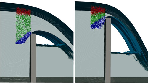
In each case, the cross-section above the weir crest was divided into three starting areas: One below the surface (A1, red), one above the weir crest (A3, blue), both with a height of 0.3 m and the last one covering the area in between (A2, green) with a height of 0.25 m in cases W4T0 and W4T2 and 1.1 m in cases W3T0 and W3T2. All particle movement simulations were started from quasi-stationary conditions, which were achieved by preliminary simulations without particles. Figure 3 shows the initialized particles, colour-coded according to the three starting areas. A simulation time of 5 s was sufficient for all particles to pass the area associated with high risk. During this time, the position of the particles, as well as their velocity and the field values pressure and velocity gradient, were stored every 0.01 s, resulting in 500 stored time steps.

Figure 3. Initial positions of the particles of the cases with a weir height of 3 m W3T2 and W3T0 (left) and of the cases with a weir height of 4 m W4T2 and W4T0 (right). Starting areas: A1 – below the surface (red; h = 0.3 m), A2 – covering the area between A1 and A3 (green; h = 0.25–1.1 m) and A3 – above the weir crest (blue; h = 0.3 m).

The primary objective of the simulation of the highly simplified overshot weir was to compare the variants that comply with the DWA tailwater criterion with those that do not. In addition, the starting areas of the individual variants were compared with each other. A statistical analysis was carried out to compare the starting areas. Since a normal distribution of the results was not given in many cases, the Kruskal–Wallis test was performed to check the results of the sample set of all 12 combinations of hydraulic conditions and particle starting areas for significant differences (Kruskal and Wallis 1952). If there were significant differences between any samples, Dunn’s post-hoc test using the Bonferroni method for adjusting p values was performed with a significance level of α = 0.05 to compare the individual pairs and to identify between which pairs there were significant differences (Dunn 1964).

3.2. Results

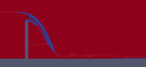
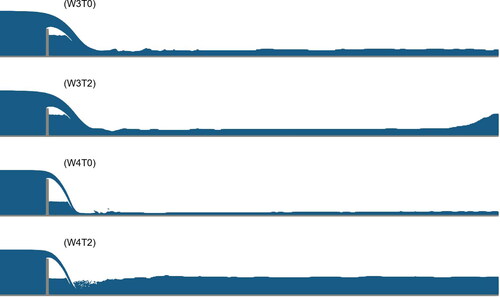
The hydraulic situations shown in Figure 4 corresponded to the expected situation. The application of Bernoulli’s principle and the calculation of the supporting forces results in a hydraulic jump migrating downstream in the case W3T2, whereas this is not the situation in the case W4T2. Accordingly, the near-fields of the weirs of W3T2 and W3T0 look very similar, but the near-fields of the weirs of W4T2 and W4T0 look distinctively different.

Figure 4. Slices through the computational domains of the four cases showing the hydraulic situations. Depicted in blue is the water-filled area. Starting from the top, W3T0 with a weir height of 3 m and a tailwater level of 0 m, W3T2 with a weir height of 3 m and a tailwater level of 2 m, W4T0 with a weir height of 4 m and a tailwater level of 0 m and W4T2 with a weir height of 4 m and a tailwater level of 2 m.

3.2.1. Shear stress

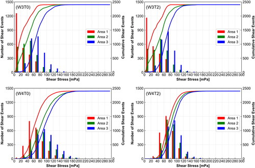
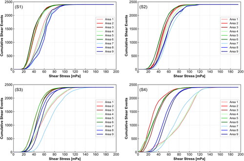
For every particle, the maximum shear stress during the downstream weir passage was recorded based on the maximum strain rate calculated over a distance of approximately 1 cm, the typical distance between a cell’s centre and its faces, and a water temperature of 20 °C. Figure 5 displays the distribution of shear stress experienced by the particles of all four cases divided into the three starting areas. Generally, the shear stress experienced by the particles of the cases with the same weir height looked similar despite different tailwater levels. In contrast, the difference between the weir heights was clearly visible despite the same tailwater levels. In all four cases, the shear stress experienced by the particles of A3 near the weir crest was relatively similar, with a peak between 60 mPa and 80 mPa for the cases with a weir height of 3 m and a peak between 80 mPa and 100 mPa for the cases with a weir height of 4 m. In contrast, the difference of the particles of A1 (close to the surface) was considerably larger. Here, almost half of all particles of the cases with a weir height of 3 m experienced shear stress below 20 mPa, whereas the peak of the cases with a weir height of 4 m was between 40 mPa and 60 mPa and 60 mPa and 80 mPa, respectively. Overall, a thicker nappe (W3T0 and W3T2) led to lower shear stresses and a more considerable variance between the starting areas than a thinner nappe (W4T0 and W4T2). The statistical analysis verified the marginal difference between adhering and not adhering to the tailwater criterion. No significant difference was found between the respective starting areas of W3T0 and W3T2 (A1: p = 1.00, A2: p = 0.50 and A3: p = 1.00), as well as the starting areas 2 of W4T0 and W4T2 (p = 1.00).

Figure 5. Sum lines and distribution of shear stress experienced by the particles. Cases W3T0 and W4T0 (left figures) have a tailwater level of 0 m, and cases W3T2 and W4T2 (right figures) of 2 m. The weir has a height of 3 m in the top row (W3T0 and W3T2) and 4 m in the bottom row (W4T0 and W4T2).

3.2.2. Pressure changes

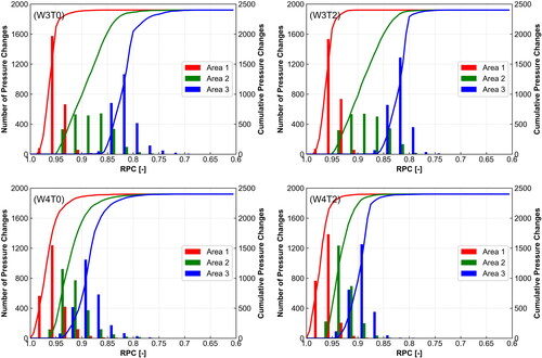
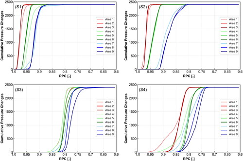
The RPC is primarily based on the initial pressure and, therefore, on the water depth at the addition position of each particle. A higher initial pressure leads to an increased pressure change and a lower RPC. The results, shown in Figure 6, reflect that very well. However, as is usual with overshot weirs, the pressure changes were generally minimal. The results of the cases W3T2 and W3T0 look very similar despite different tailwater levels. The smaller start areas A1 and A3 have distinctive peaks in the class 0.825–0.8 and 0.975–0.95, respectively, correlating with their respective depths, whereas the RPCs of the wider A2 are stretched between the former. W4T2 and W4T0 were very similar as well, but due to the thinner nappe, the results of the different starting areas were much closer together.

Figure 6. Sum lines and distribution of pressure changes experienced by particles. Cases W3T0 and W4T0 (left figures) have a tailwater level of 0 m, and cases W3T2 and W4T2 (right figures) of 2 m. The weir has a height of 3 m in the top row (W3T0 and W3T2) and 4 m in the bottom row (W4T0 and W4T2).

3.2.3. Collision

For evaluating the tailwater criterion, collisions were of primary concern.

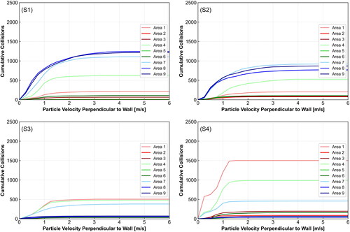
Because for each particle, only the collision with the highest velocity was recorded, the total number of collisions can only be as high as the number of particles, which was 2401 per starting area. Figure 7 displays the number of collisions in relation to the particle’s velocity perpendicular to the wall right before the recorded collision. Again, there was a substantial difference between the 3 m and 4 m weir height cases, whereas the differences between the 0 m and 2 m tailwater levels were much more subtle. This is particularly prevalent for the number of collisions of particles of A1 in each case. For case W3T2, no collision (0.0% of particles) and for case W3T0, eight collisions (0.3% of particles) were recorded for the particles of A1. For case W4T2, 1284 collisions (53.5% of particles) and for case W4T0, 1109 collisions (46.2% of particles) were recorded. Also, for the particles near the weir crest of A3, the recorded collision numbers were higher for cases W4T2 and W4T0 than for cases W3T2 and W3T0.

Figure 7. Sum lines and distribution of particle velocities perpendicular to the wall before recorded collisions. Cases W3T0 and W4T0 (left figures) have a tailwater level of 0 m, and cases W3T2 and W4T2 (right figures) of 2 m. The weir has a height of 3 m in the top row (W3T0 and W3T2) and 4 m in the bottom row (W4T0 and W4T2).

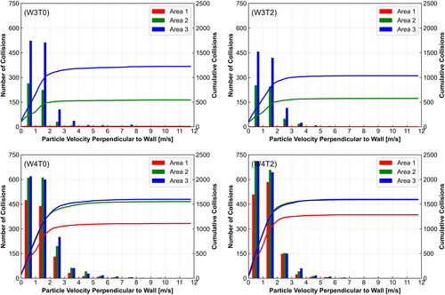
Whereas the number of collisions can be pretty high, the particles’ velocities perpendicular to the wall before the recorded collisions were relatively low. In all cases, most collisions occured at a velocity of less than 2 m/s towards the wall (W3T0: 86.3%, W3T2: 85.3%, W4T0: 78.8% and W4T2: 85.4%). In the cases with a weir height of 4 m, the difference between the tailwater cushions was more relevant than in those with a weir height of 3 m. This is reflected as well in the statistical analysis of the velocities. Dunn’s test showed no significant difference between the respective starting areas with collisions of W3T2 and W3T0 (A2: p = 1.00, A2: p = 1.00). In contrast, the differences between the respective starting areas of W4T2 and W4T0 are significant (A1: p = 0.00, A2: p = 0.00 and A3: p = 0.00).

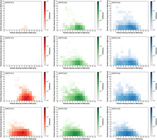
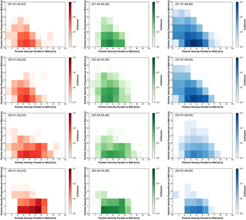
The forces acting on a fish when struck perpendicular to the surface are much greater than when struck at a very acute angle. Also, a fish may have a higher opportunity to avoid a collision at a narrow angle by active movement than a collision at a wide angle because the velocity in the direction to the solid surface is considerably lower. Still, the velocity parallel to the wall before the impact can be of relevance as well. Figure 8 shows heatmaps of all collisions, divided according to the velocities parallel and perpendicular to the wall.

Figure 8. Number of recorded collisions divided according to the particle velocity perpendicular and parallel to the wall before the collision. From top to bottom: W3T0 (weir height 3 m, tailwater level 0 m), W3T2 (weir height 3 m and tailwater level 2 m), W4T0 (weir height 4 m and tailwater level 0 m), W4T2 (weir height 4 m and tailwater level 2 m). The first column (red) is starting area 1, the second column (green) starting area 2 and the third column (blue) starting area 3.

Of further interest is the location of the collisions. Due to the discrete particle tracking every 0.01 s and the collision detection method, particles can be up to roughly 5 cm from the next wall when a collision is detected. In addition, collision detection is strongly dependent on grid discretization. Figure 9 shows the locations of all recorded collisions of case W4T2. Since the collision positions are comparable in all four cases, W4T2 was selected as representative and is presented here. Accordingly, the following statements are valid for all cases. The positions of the collisions matched the flow pattern very well. In the area where the nappe hits the bottom, most collisions occurred, and the impact velocities were highest. In the peripheral areas, the impact velocities were generally lower. The abrupt end of the recorded collision points is striking. This is due to the end of the cell refinement area. With the larger cells of 8 cm, the centre of all cells is more than 2 cm from the wall, and collisions are no longer detected. This was a deliberate choice. Because of the hydraulic situation, no further relevant collisions were expected.

Figure 9. Locations and impact velocities of all recorded collisions of case W4T2. The velocity is plotted on the background. The cell size is visible on the bottom.

4. Case study: Pulverweiden weir

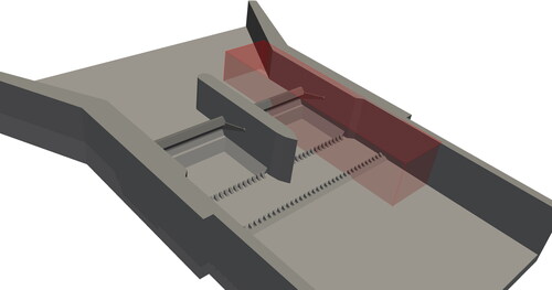
To test the applicability of the method described, a case study was conducted. The method was applied to the weir Pulverweiden on the river Saale in Germany. Pulverweiden weir consists of two identical and symmetrical weir openings with segment gates of 17.5 m in width. A special feature of the system is that the segment gates can be raised as well as lowered. Accordingly, the weir is operated as an overshot weir during low flows and an undershot weir during high flows. The mean water flow is around 50 m³/s and the drop height is slightly above 2 m, depending on the flow situation. This weir was chosen as a test case because, on the one hand, it is possible to examine overshot and undershot situations at one weir, and even though the drop height is relatively low, potentially harmful situations for fish cannot be ruled out due to two rows of baffle blocks at the end of the stilling basin. On the other hand, due to the relatively simple geometry, Pulverweiden weir is an ideal test case.

The aim of this case study is not a final damage potential analysis but rather the verification of the method’s applicability to real weirs. The questions to be answered are what results this method can deliver and what potential exists.

4.1. Model description

Due to the identical and symmetrical weir openings, only half of one weir opening is depicted in the numerical model in order to reduce the computational effort drastically. Because of the symmetrical design, this simplification only leads to a slight deviation, which was accepted. The model has dimensions of 45.12 m in length, 10.24 m in width and 10 m in height. The weir was placed at about one-third of the model, resulting in an upstream length of 15 m and a tailwater length of 30 m. The dimensions of the model area are shown in Figure 10.

Figure 10. The geometry of the Pulverweiden weir with two segment gates, the stilling basin and two rows of baffle blocks. Headwater on the left and tailwater on the right. The red box indicates the model area.

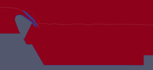
With a base cell length of 32 cm and an iterative refinement down to a cell edge length of 2.0 cm along all walls, the nappe and the area of possible particle movement, the computational grid consists of 50 million to 60 million cubic cells, depending on the gate position. To avoid differing measured shear stress due to varying cell size, no wall layers were added. As in the first test case, a mesh independence analysis was performed with five different mesh refinements with cell lengths of 16.0, 8.0, 4.0, 2.0 and 1.0 cm in the areas of high flow gradients and possible particle movement. As the flow rate was defined to be constant, the headwater level as well as the simulated turbulence share as an LES quality criterion was evaluated. Compared to the situation with a cell length of 1.0 cm, the mean headwater level barely deviated by 0.07 cm (cell length 2.0 cm), 0.46 cm (4.0 cm), 0.35 cm (8.0 cm) and 0.25 cm (16.0 cm). Figure 11 shows the plunge pool of the case with a cell length of 2.0 cm. In the red areas, at least 80% of the turbulent kinetic energy is simulated and less than 20% is modelled by sub-grid models. This is not the case in the blue areas. Except for the phase interface of the nappe, this criterion for good LES is fulfilled. As the added particles have to be smaller than the cells to avoid unphysical behaviour, the coarsest grid was selected, which represents the hydraulic situation sufficiently well.

Figure 11. Section of the calculation area with a cell length of 2.0 cm. In red: Areas in which at least 80 % of the turbulent kinetic energy is simulated and less than 20 % is modelled by Sub-grid models. In blue: Areas in which more than 20 % is modelled. The white lines represent the water surface.

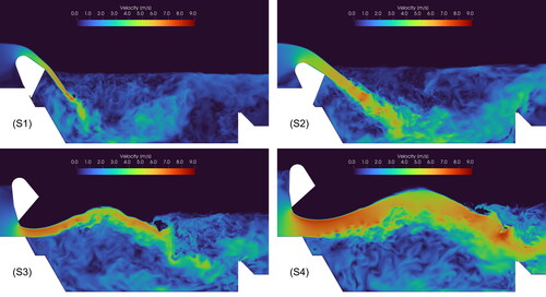
Four different flow situations and correspondingly different weir positions were examined. The first situation (S1) depicts a frequently recurring mean flow with a total discharge of 50 m³/s. In this situation, the weir is operated as an overshot weir. The second (S2) and third (S3) situations had the same total discharge of 110 m³/s. At this discharge, the operation mode is changed from overshot (S2) to undershot (S3). The fourth selected situation (S4) depicts an average flood discharge of 240 m³/s. Here, the weir is operated as an undershot weir. Figure 12 shows slices of the four situations at the beginning of the simulation. The boundary conditions are identical to those of the first test case except for the inlet and the left wall. At the inlet a volume flow is defined, the water level sets freely. To the left the domain is confined by the weir side wall and therefore defined as rough wall (no-slip).

Figure 12. Initial flow conditions of the four situations considered. In the first two cases (top), the weir is operated as an overshot weir and in the two later cases (bottom), the weir is operated as an undershot weir. The water velocity is plotted on the slice.

In contrast to the first case study, there is a possible variance in the fate of migrating fish based on their horizontal position due to the solid wall on one side. Therefore, the starting areas were not only divided vertically in three sections but also horizontally in three sections, resulting in nine starting areas. These were numbered starting from the wall. The height of the starting areas next to the surface (A1–A3), as well as the areas next to the weir crest (A7–A9), is around one-third of the total depth but no more than 0.3 m. The starting areas horizontally in the middle (A4–A6) occupy the remaining space, which is from 0.2 m up to 0.9 m, depending on the gate position. After an initialization simulation without particles to create quasi-stationary initial conditions, 2401 particles were initiated per starting area. A simulation time of 10 s was sufficient for all particles to pass the area associated with high risk. During this time, the position of the particles, their velocity and the field values pressure and velocity gradient were stored every 0.01 s, resulting in 1000 stored time steps.

For the assessment of the damage potential, a quantitative evaluation is necessary. In addition, the four situations are to be compared qualitatively, particularly those with the same discharge but different operating modes (S2 overshot and S3 undershot). As with the simplified test case, shear stress, pressure changes and collisions were analysed and described separately. As the comparison of the individual starting ranges was not the main focus of this investigation, the statistical analysis was omitted.

4.2. Results

4.2.1. Shear stress

The highest shear stress was recorded for every particle during the simulation based on the strain rate over a distance of approximately 1 cm, the typical distance between a cell’s centre and its faces, and a water temperature of 20 °C. Figure 13 displays the shear stress experienced by the particles of all four situations divided into the nine starting areas. Generally, there was a perceptible difference between the situations with overflowed and underflowed weirs. The shear stress experienced by the particles of all starting areas of S1 and S2 (overshot) was roughly in the same range with mean values between 39 mPa (A6) and 60 mPa (A8) and between 45 mPa (A5) and 60 mPa (A7), respectively. Particles that start close to the weir body or the wall experienced slightly higher shear stress (A1, A4 and A7–A9). 80% of all recorded values of all starting areas of S1 and S2 were between 25 mPa and 86 mPa. The shear stress experienced by the particles of the starting areas of S3 and S4 (undershot) differed much more. Especially, the starting areas next to the wall (A1, A4 and A7) experienced higher shear stress. The mean values of S04 were between 30 mPa (A2) and 83 mPa (A1). 80% of all recorded values of all starting areas of S3 and S4 are between 9 mPa and 115 mPa. In the undershot situations, the vertical distribution affected less the shear stress experienced.

Figure 13. Sum lines of shear stress experienced by the particles. Cases S1 and S2 (top figures) are overshot situations, and cases S3 and S4 (bottom figures) are undershot situations. The discharge increases from 50 m³/s (S1) to 110 m³/s (S2 and S3) and 240 m³/s (S4).

4.2.2. Pressure changes

As in the first test case, there was a clear correlation between the initial pressure, i.e. the initial depth of the particle, and the RPC. A higher initial pressure led to an increased pressure change and a lower RPC. The RPCs of all four simulated situations are depicted in Figure 14. Particles of starting areas in a horizontal row experienced virtually the same pressure changes. Vertically, more substantial pressure fluctuations can be observed with increasing initial depth. In all situations, particles of the lower starting areas A7–A9 experienced the strongest pressure changes and particles of the upper starting areas A1–A3 the smallest pressure changes. The difference between the overshot (S1 and S2) and undershot (S3 and S4) situations is evident. Whereas the mean RPCs of S1 and S2 were above 0.9 (0.94 and 0.92, respectively), particles in undershot situations experienced a mean RPC of 0.79 (S3) and 0.80 (S4). 80% of all recorded RPCs of all starting areas of the overshot situations (S1 and S2) were between 0.98 and 0.83, and of the undershot situations (S3 and S4) between 0.91 and 0.74.

Figure 14. Sum lines of pressure changes experienced by the particles. Cases S1 and S2 (top figures) are overshot situations, and cases S3 and S4 (bottom figures) are undershot situations. The discharge increases from 50 m³/s (S1) to 110 m³/s (S2 and S3) and 240 m³/s (S4).

4.2.3. Collision

Due to the modest water level difference of Pulverweiden weir, collisions were of primary concern. Because for each particle, only the collision with the highest velocity was recorded, the total number of collisions can only be as high as the number of particles, which is 2401 per starting area. Figure 15 displays the number of collisions in relation to the particle’s velocity perpendicular to the wall right before the recorded collision. Differences can be observed between situations and the individual starting fields of the situations. There was a clear difference between starting fields close to the wall (A1, A4 and A7) and the weir body in overshot situations (A7–A9) with over 2000 collisions each (21.9 − 25.3% of particles) and the open water starting fields (A2, A3, A5 and A6) with less than 500 collisions each (2.0 − 4.2% of particles). In the overshot situations (S1 and S2), most collisions occured at the lower starting fields A7–A9, and in the undershot situations (S3 and S4) at the starting fields near the lateral wall (A1, A4 and A7). Overall, the velocities perpendicular to the wall before the recorded collisions were low. The mean values were between 0.5 m/s and 1.5 m/s, and the 90th percentiles were between 1 m/s and 2.5 m/s. The velocities were particularly low for collisions of the starting fields near the lateral wall.

Figure 15. Sum lines of particle velocities perpendicular to the wall before recorded collisions. Cases S1 and S2 (top figures) are overshot situations, and Cases S3 and S4 (bottom figures) are undershot situations. The discharge increases from 50 m³/s (S1) to 110 m³/s (S2 and S3), and 240 m³/s (S4).

An additional look at the velocities parallel to the wall, shown in Figure 16, reveals that these were comparable across all situations and starting areas. Most collisions occured at a velocity parallel to the wall between 2 m/s and 6 m/s. In situations S1–S3, the greatest accumulation was between 3 m/s and 4 m/s, in situation S4 between 4 m/s and 5 m/s. It can also be seen in this representation that the velocities perpendicular to the wall were lowest for collisions in situation S4. Here, collisions with the side wall dominated, characterized by small impact angles and, therefore, low velocities against the wall.

Figure 16. Number of recorded collisions divided according to the particle velocity perpendicular and parallel to the wall before the collision. Cases S1 and S2 (upper figures) are overshot situations, and cases S3 and S4 (lower figures) are undershot situations. The first column (red) is the upper starting areas A1–A3, the second column (green) the Middle starting areas A4–A6, and the third column (blue) is the lower starting areas A7–A9.

5. Discussion

In the context of this work, several of aspects were highlighted and two test cases were carried out, which differ significantly in their approach. Accordingly, the discussion is divided into three parts:

1. The applicability of the tailwater criterion will be evaluated using the simplified overshot weir.

2. The results of the simulations of the Pulverweiden weir will be used to assess the damage potential of the weir on fish.

3. The practicability of the presented method, its potential and existing problems will be discussed.

5.1. Tailwater criterion

The aim is to evaluate the usability of the tailwater criterion for the assessment of downstream fish passage over weirs. Since the hydraulic situation at a weir differs significantly from a bypass as described, the nappe displaces the tailwater cushion that is supposed to avoid collisions. On the other hand, a water cushion builds up between weir and nappe due to the momentum equilibrium. This has already been observed in previous studies (Thorenz et al. 2018).

The results of this work confirm these observations. The number of collisions is almost unaffected by whether there is a theoretically sufficient tailwater level. This is not surprising when comparing cases W3T0 and W3T2. Due to the downstream migration of the hydraulic jump, the flow is supercritical in the potentially harmful area and, therefore, unaffected by the downstream water level. In these cases, the application of the tailwater criterion is not reasonable. Nevertheless, when comparing cases W4T0 and W4T2, there is an influence of the tailwater level. The number of collisions is not significantly reduced, but the impact velocities are. The mean particle velocities before a collision are significantly lowered by roughly 1.5–2 m/s, depending on the starting area. Although the number of collisions is relatively high, it is necessary to note that the impact angles are very small in most cases. An impact with very low velocity perpendicular to the surface is certainly less severe than with high velocity. A particular effect of the tailwater cushion on the impact angles was noticeable. Where in case W4T0, 12 collisions were detected with particle velocities of 8–10 m/s perpendicular to the wall, none of the collisions in case W4T2 occurred at more than 8 m/s. However, since there is no discernible influence on the majority of the particles, no significant correlation could be identified.

Despite the slight reduction of impact velocities, the tailwater criterion does not seem to be able to identify acceptable situations in many cases. Also, increasing the required water cushion in relation to the height difference does not appear to be effective. In the cases considered, a tailwater level of 70% of the drop height only had a marginal effect. The situation, which is substantially different from the bypass, requires other criteria in order to ensure an acceptable situation for downstream fish passage. Depending on the starting position of the particle, the thickness of the nappe showed a noticeable influence. For particles starting in the lower areas, the thickness of the nappe had no significant influence. For particles starting in the higher areas, the thicker nappe led to an almost complete prevention of collisions.

5.2. Damage potential weir Pulverweiden

The validity of a quantitative damage potential estimate relies on the sufficient fulfilment of five steps: (1) The precise depiction of the hydraulic situation around the weir and the tailwater area; (2) The movement of the particles must be simulated accurately using the Lagrangian method; (3) Determining the hydraulic stressors from the numerical simulation has to be correct; (4) The transferability of the particles to fish must be given; (5) The effects of the hydraulic stressors on fish have to be known.

The extent to which these criteria are met diminishes in descending order. The applied numerical method to simulate the fluid flow field is a proven tool used for scientific purposes for many years (Deshpande et al. 2013; Gisen et al. 2017; Thorenz et al. 2018). Despite certain simplifications, a good representation of the hydraulic situation can be assumed with a conscientious and trained application. The particle movement is subject to more remarkable simplifications and has not been proven to the same extent. Nevertheless, the most important influencing variables are considered. The evaluation of pressure, shear stress and collisions are influenced by the recording method and the grid discretization. This will be further elaborated in the following section. Complete transferability of the movement and behaviour of the particles to fish is not given. This also differs greatly among different fish with different body shapes and sizes. Accordingly, no single particle can represent an exact fish, but the totality of particles can approximate the movement and distribution of passively moving fish. Finally, the effect of hydraulic stressors, especially their interaction, is largely unknown. For individual fish in certain life stages, dose-response dependencies are known under specific laboratory conditions, but this can only serve as a rough indicator.

In conclusion, no comprehensive quantitative assessment of the damage potential of the Weir Pulverweiden is currently feasible. Nevertheless, a rough estimate based on the results of its CFD simulation can be done. However, this estimation should be viewed with caution, taking into account the uncertainties. For the most part, the maximum shear stress experienced by the particles is between 40 mPa and 80 mPa, with the highest values recorded below 140 mPa, corresponding to a strain rate of 140 s⁻¹. In the literature, the first injuries to fish are reported at strain rates of 339 s⁻¹ based on a distance of 1.8 cm (Colotelo et al. 2018). Due to differing observation distances, partly unclear and synonymous use of shear, shear stress and strain rate, as well as difficult measurement of shear, it is difficult to draw a clear conclusion. However, despite the uncertainties, the shear rates recorded appear to be far from injury thresholds for fish.

The pressure changes measured are also within a range that is considered harmless for fish. Although they are greater in the undershot situations, the RPC is in any case above the value of 0.7, which is assumed to be safe by Čada and Charles (1997) and Boys et al. (2016a), even considering sensitive fish species.

A substantial amount of collisions were recorded, especially for starting areas close to the wall. Overall, the particle velocities before the collisions, especially perpendicular to the wall, were low. Only in 2.1% of all collisions was the velocity perpendicular to the wall above 3 m/s and in none above 5 m/s, corresponding to a mortality rate of 0% according to the USACE (1991). However, this consideration neglects the velocity parallel to the wall. Further knowledge about the effects of these situations is necessary for a quantitative assessment. When comparing S02 and S03, it can be said that in this case, overshot operation leads to a higher number of collisions, but undershot operation leads to slightly higher pressure changes.

5.3. Practicability, potentials and problems

The method testing based on two test cases should show to what extent the presented method is applicable for investigating downstream fish passage over a weir. In general, the method is very promising for the estimation and qualitative comparison of different situations. One advantage arises from the fact that it is based on the frequently used two-phase solver interFoam and can be easily applied to existing cases. Adding the simple particles and the one-way coupling also did not lead to stability problems or significantly increased computing times. This method allows a quick and numerically stable way of simulating high numbers of strictly spherical particles, but not a more sophisticated depiction of a specific fish. However, as each fish has many individual characteristics like shape, size and flexibility, representing every fish is an impossible task. Therefore, the simulation of a large number of simple spherical particles with the corresponding simplifications was chosen.

The significant hydraulic stressors shear stress, pressure changes and collisions can be evaluated, but not secondary factors, such as increased predation. The evaluation of the pressure changes is done very simply via the instantaneous pressure in the cell in which the particle is located. Since the pressure fluctuation depends almost exclusively on the acclimatization pressure, i.e. the water depth before the passage, an estimation without numerical simulation is also possible.

The shear stress is also determined via the cell in which the particle is located. However, there is an influence due to the grid discretization. Comparability with experimental data with different reference lengths is tricky. The measured value also depends on the coordinate system. The actual value can be up to $\sqrt{2}$ times higher. Therefore, only a rough order of magnitude and not an exact value is obtained.

Collision detection was carried out similarly to autonomous sensor devices for field operations via the velocity change. Several artificial boundaries are drawn here. First, the threshold of acceleration above which a collision is registered. Here, a threshold of 10 g was chosen. Furthermore, a collision is only assumed if a particle is close to a wall. This is determined by the cell in which the particle is located. The centre of this cell must be less than 0.04 m from the nearest wall for a collision to be registered. This leads to two detected artefacts in the collision evaluation. First, the cell size again has a clear impact. If the cell size reaches an edge length of 0.08 m, collisions are no longer detected. This can be used to define the area under consideration. Second, collisions can be registered even if no actual collision took place. If a particle moves close to a wall and is decelerated or accelerated, a collision is detected. This can be applied to infer larger fish from tiny particles by setting the necessary distance to the wall. Finally, the collision detection method also affects the detected impact angle. If a particle moves at a minimal angle towards a wall, the collision can be detected a few time steps before the actual impact. Since no deflection has taken place at this point, the impact angle is close to zero. In practice, it has been shown that in some collisions, the angle of impact is distorted from about 5°−10° to almost 0°. This alteration is visible in the impact angle figures as a gap between collisions with impact angles close to zero and larger impact angles. However, because only small angles are altered slightly, it is insignificant.

Something that has proved to be important in the test cases is the separation into different starting areas. These can have a significant impact on the results. The more starting areas, the more detailed the result. However, the necessary number of starting areas is also strongly dependent on the case’s complexity. For the quasi-two-dimensional test case, three start areas were sufficient; the real weir required more. However, the test cases also showed the method has weaknesses in real situations. Flows parallel to walls, as found on the sides in real situations, led to many collisions that are difficult to evaluate. This is not the case with cut-out models. Without extensive validation and more knowledge about the effects of collisions at small impact angles on fish and whether they can be prevented by active swimming, it is preferable to limit the focus to basic research rather than assessing real-life situations.

6. Conclusion

In this study, two test cases, a simplified weir and the actually existing Pulverweiden weir, were simulated using the open-source CFD library OpenFOAM^® and an adapted solver based on the two-phase solver interFoam, extended with Lagrangian particles to represent passively transported fish. Each test case consisted of four simulated situations. The simplified weir was simulated with two different weir heights, each with two different tailwater levels. Four flow situations were simulated for the Pulverweiden weir.

Recommendations regarding the necessary tailwater level for downstream fish passage over weirs were reviewed. The results of the simulations show that adherence to the recommendation of a tailwater level of a quarter of the water level difference, but at least 0.9 m (DWA 2021), has no significant impact on the relevant hydraulic stressors in certain situations. The number of collisions is independent of the underwater level; in some cases, impact velocities can be slightly reduced. The thickness of the nappe has a significantly greater influence. A thick nappe leads to a significant reduction in collisions, especially of particles initialized near the surface. This result confirms the concern that the abovementioned recommendation for the tailwater level does not prove to be able to identify safe downstream passage of fish over the weir.

Due to the unsatisfactory state of knowledge on fish descent via weirs, further intensive investigations are necessary. The CFD method used in this study is suitable for this purpose with certain limitations. A general advantage of the downstream particle trajectory evaluation is that it is based on the frequently used solver interFoam. It is not necessary to constantly maintain a separate solver. The disadvantage is the limited performance of the Python post-processing and the large amounts of data generated. Limitations exist due to the depiction of the fish as small spherical particles, the measurement of hydraulic stressors and unknown dose-response dependencies. Accordingly, qualitative comparisons of different situations are possible, but not the determination of the damage potential of a specific situation.

Going forward, CFD simulations using passive particles can help to understand the downstream fish passage over weir structures better. Factors influencing the safety of downstream migration can be recognized, and adapted recommendations for the design and operation of weirs can be developed. In order to conduct detailed damage analyses, further research in two directions is important. On the one hand, the validation of the CFD methodology is necessary. This concerns the simplification of the representation of fish as well as the particle movement in general. On the other hand, a more comprehensive knowledge of dose-response dependencies is necessary to be able to translate the results of the numerical simulations into actual damage rates.

Disclosure statement

No potential conflict of interest was reported by the author(s).

References

- Abernethy C, Amidan B, Cada G. 2001. Laboratory studies of the effects of pressure and dissolved gas supersaturation on Turbine-Passed Fish. Richland (WA): Pacific Northwest National Laboratory.
- Abernethy C, Amidan B, Cada G. 2002. Simulated passage through a modified Kaplan turbine pressure regime: a supplement to “laboratory studies of the effects of pressure and dissolved gas supersaturation on turbine-passed fish”. Richland (WA): Pacific Northwest National Laboratory.
- Adam B, Lehmann B. 2011. Ethohydraulik: grundlagen, Methoden und Erkenntnisse. Berlin, Germany: Springer.
- Andrews MJ, O'Rourke PJ. 1996. The multiphase particle-in-cell (MP-PIC) method for dense particulate flows. Int J Multiph Flow. 22(2):379–402.
- Barbarossa V, Schmitt RJP, Huijbregts MAJ, Zarfl C, King H, Schipper AM. 2020. Impacts of current and future large dams on the geographic range connectivity of freshwater fish worldwide. Proc Natl Acad Sci USA. 117(7):3648–3655. doi: 10.1073/pnas.1912776117.
- Baumgartner LJ, Daniel Deng Z, Thorncraft G, Boys CA, Brown RS, Singhanouvong D, Phonekhampeng O. 2014. Perspective: towards environmentally acceptable criteria for downstream fish passage through mini hydro and irrigation infrastructure in the Lower Mekong River Basin. J Renew Sustain Energy. 6(1):12301.
- Baumgartner LJ, Reynoldson N, Gilligan DM. 2006. Mortality of larval Murray Cod (Maccullochella peelii peelii) and Golden Perch (Macquaria ambigua) associated with passage through two types of low-head weirs. Mar Freshw Res. 57(2):187–191.
- Baumgartner LJ, Thorncraft G, Phonekhampheng O, Boys C, Navarro A, Robinson W, Brown R, Deng ZD. 2017. High fluid shear strain causes injury in Silver Shark: preliminary implications for Mekong hydropower turbine design. Fish Manag Ecol. 24(3):193–198.
- Bell M, DeLacy A. 1972. A compendium on the survival of fish passing through spillways and conduits. Portland (OR): US Army Corps of Engineers.
- Belletti B, Garcia de Leaniz C, Jones J, Bizzi S, Börger L, Segura G, Castelletti A, van de Bund W, Aarestrup K, Barry J, et al. 2020. More than one million barriers fragment Europe’s rivers. Nature. 588(7838):436–441. doi: 10.1038/s41586-020-3005-2.
- Benigni H, Schneider J, Reckendorfer W, Jaberg H, Zenz G, Tuhtan J. 2021. Numerical simulation and experimental verification of downstream fish migration in a Kaplan turbine. IOP Conf Ser: earth Environ Sci. 774(1):012149. doi: 10.1088/1755-1315/774/1/012149.
- Benigni H, Schneider J, Reckendorfer W, Schiffer J, Tuhtan J, Leithner S, Zenz G, Meusburger P. 2022. Numerical simulation and experimental verification of downstream fish migration in a Bulb turbine. IOP Conf Ser: earth Environ Sci. 1079(1):012101. doi: 10.1088/1755-1315/1079/1/012101.
- Boys C, Baumgartner L, Miller B, Deng Z, Brown R, Pflugrath B. 2013. Protecting downstream migrating fish at mini hydropower and other river infrastructure. Nelson Bay, Australia: NSW Department of Primary Industry.
- Boys C, Navarro A, Robinson W, Fowler A, Chilcott S, Pflugrath B, Baumgartner L, McPherson J, Brown R, Deng Z. 2014. Downstream fish passage criteria for hydropower and irrigation infrastructure in the Murray–Darling Basin. Nelson Bay, Australia: NSW Department of Primary Industries.
- Boys CA, Robinson W, Miller B, Pflugrath B, Baumgartner LJ, Navarro A, Brown R, Deng Z. 2016a. A piecewise regression approach for determining biologically relevant hydraulic thresholds for the protection of fishes at river infrastructure. J Fish Biol. 88(5):1677–1692.
- Boys CA, Robinson W, Miller B, Pflugrath B, Baumgartner LJ, Navarro A, Brown R, Deng Z. 2016b. How low can they go when going with the flow? Tolerance of egg and larval fishes to rapid decompression. Biol Open. 5(6):786–793. doi: 10.1242/bio.017491.
- Brackbill J, Kothe D, Zemach C. 1992. A continuum method for modeling surface tension. J Comput Phys. 100(2):335–354.
- Brown RS, Carlson TJ, Gingerich AJ, Stephenson JR, Pflugrath BD, Welch AE, Langeslay MJ, Ahmann ML, Johnson RL, Skalski JR, et al. 2012. Quantifying mortal injury of juvenile Chinook Salmon exposed to simulated hydro-turbine passage. Trans Am Fish Soc. 141(1):147–157. doi: 10.1080/00028487.2011.650274.
- Brown RS, Colotelo AH, Pflugrath BD, Boys CA, Baumgartner LJ, Deng ZD, Silva LGM, Brauner CJ, Mallen-Cooper M, Phonekhampeng O, et al. 2014. Understanding barotrauma in fish passing hydro structures: a global strategy for sustainable development of water resources. Fisheries. 39(3):108–122. doi: 10.1080/03632415.2014.883570.
- Čada G, Carlson T, Ferguson J, Richmond M, Sale M. 1999. Exploring the role of shear stress and severe turbulence in downstream fish passage. Paper presented at: Waterpower Conference. Hydro’s future: technology, markets and policy; July 6–9, 1999; Las Vegas (NV). Reston (VA): American Society of Civil Engineers; p. 1–9.
- Čada G, Charles C. 1997. Development of biological criteria for the design of advanced hydropower turbines. Oak Ridge (TN): Oak Ridge National Laboratory.
- Čada GF. 1990. A review of studies relating to the effects of propeller-type turbine passage on fish early life stages. N Am J Fish Manag. 10(4):418–426.
- Čada GF. 2001. The development of advanced hydroelectric turbines to improve fish passage survival. Fisheries. 26(9):14–23. doi: 10.1577/1548-8446(2001)026<0014:TDOAHT>2.0.CO;2.
- Čada GF. 2007. Determining the effect of shear stress on fish mortality during turbine passage. Hydro Rev. 26(7):52.
- Carlson TJ, Brown RS, Stephensons JR, Gingerich AJ, Pflugrath BD, Colotelo AH, Welch AE, Benjamin PL, Skalski JR, Seaburg AG, et al. 2010. Assessment of barotrauma in untagged and tagged juvenile Chinook Salmon exposed to simulated hydro turbine passage. Richland (WA): Pacific Northwest National Laboratory.
- Colotelo AH, Mueller RP, Harnish RA, Martinez JJ, Phommavong T, Phommachanh K, Thorncraft G, Baumgartner LJ, Hubbard JM, Rhode BM, et al. 2018. Injury and mortality of two Mekong River species exposed to turbulent shear forces. Mar Freshw Res. 69(12):1945.
- Cox RX, Kingsford RT, Suthers I, Felder S. 2023. Fish injury from movements across hydraulic structures: a review. Water. 15(10):1888. doi: 10.3390/w15101888.
- Dauble DD, Deng Z, Richmond MC, Moursund RA, Carlson TJ, Rakowski CL, Duncan JP. 2007. Biological assessment of the advanced turbine design at Wanapum Dam, 2005. Richland (WA): Pacific Northwest National Laboratory.
- Dedual M. 2007. Survival of juvenile Rainbow Trout passing through a Francis turbine. N Am J Fish Manag. 27(1):181–186.
- Deng Z, Carlson TJ, Dauble DD, Ploskey GR. 2011. Fish passage assessment of an advanced hydropower turbine and conventional turbine using blade-strike modeling. Energies. 4(1):57–67. doi: 10.3390/en4010057.
- Deng Z, Guensch GR, McKinstry CA, Mueller RP, Dauble DD, Richmond MC. 2005. Evaluation of fish-injury mechanisms during exposure to turbulent shear flow. Can J Fish Aquat Sci. 62(7):1513–1522.
- Deng Z, Mueller RP, Richmond MC, Johnson GE. 2010. Injury and mortality of juvenile salmon entrained in a submerged jet entering still water. N Am J Fish Manag. 30(3):623–628.
- Deng ZD, Lu J, Myjak MJ, Martinez JJ, Tian C, Morris SJ, Carlson TJ, Zhou D, Hou H. 2014. Design and implementation of a new autonomous sensor fish to support advanced hydropower development. Rev Sci Instrum. 85(11):115001.
- Deshpande SS, Anumolu L, Trujillo MF. 2013. Evaluating the performance of the two-phase flow solver interFoam. Comput Sci Disc. 5(1):014016.
- Doyle KE, Ning N, Silva LGM, Brambilla EM, Boys CA, Deng ZD, Fu T, Du Preez JA, Robinson W, Baumgartner LJ. 2020. Gambusia holbrooki survive shear stress, pressurization and avoid blade strike in a simulated pumped hydroelectric scheme. Front Environ Sci. 8:1–14. doi: 10.3389/fenvs.2020.563654.
- Doyle KE, Ning N, Silva LGM, Brambilla EM, Deng ZD, Fu T, Boys C, Robinson W, Du Preez JA, Baumgartner LJ. 2022. Survival estimates across five life stages of Redfin (Perca fluviatilis) exposed to simulated pumped-storage hydropower stressors. Conserv Physiol. 10(1):coac017. doi: 10.1093/conphys/coac017.
- Duncan JP. 2013. Characterization of fish passage conditions through the fish weir and turbine unit 1 at Foster Dam, Oregon, using Sensor Fish, 2012. Richland (WA): Pacific Northwest National Laboratory.
- Dunn OJ. 1964. Multiple comparisons using rank sums. Technometrics. 6(3):241–252. doi: 10.1080/00401706.1964.10490181.
- DWA. 2005. Fischschutz- und Fischabstiegsanlagen: bemessung, Gestaltung, Funktionskontrolle. Hennef (Germany): DWA Dt. Vereinigung für Wasserwirtschaft Abwasser und Abfall.
- DWA. 2021. Methodische Grundlagen zur standörtlichen Evaluierung des Fischschutzes und Fischabstiegs. Hennef (Germany): Deutsche Vereinigung für Wasserwirtschaft Abwasser und Abfall.
- Ebel G. 2013. Fischschutz und Fischabstieg an Wasserkraftanlagen: fish protection and downstream passage at hydro Power stations; Handbuch Rechen- und Bypasssysteme. Halle (Saale) (Germany): Büro für Gewässerökologie und Fischereibiologie Dr. Ebel.
- Ebel G. 2014. Modellierung der Schwimmfähigkeit europäischer Fischarten—Zielgrößen für die hydraulische Bemessung von Fischschutzsystemen. Wasserwirtschaft. 104(7-8):40–47. doi: 10.1365/s35147-014-1095-1.
- Elghobashi S. 1994. On predicting particle-laden turbulent flows. Appl Sc Res. 52(4):309–329.
- Eyler SM, Welsh SA, Smith DR, Rockey MM. 2016. Downstream passage and impact of turbine shutdowns on survival of Silver American Eels at five hydroelectric dams on the Shenandoah River. Trans Am Fish Soc. 145(5):964–976. doi: 10.1080/00028487.2016.1176954.
- Feathers MG, Knable AE. 1983. Effects of depressurization upon Largemouth Bass. N Am J Fish Manag. 3(1):86–90.
- Fernandes C, Semyonov D, Ferrás LL, Nóbrega JM. 2018. Validation of the CFD-DPM solver DPMFoam in OpenFOAM® through analytical, numerical and experimental comparisons. Granul Matter. 20(4):64.
- Foye RE, Scott M. 1965. Effects of pressure on survival of six species of fish. Trans Am Fish Soc. 94(1):88–91.
- Fu T, Deng ZD, Duncan JP, Zhou D, Carlson TJ, Johnson GE, Hou H. 2016. Assessing hydraulic conditions through Francis turbines using an autonomous sensor device. Renew Energ. 99:1244–1252.
- Gisen DC, Weichert RB, Nestler JM. 2017. Optimizing attraction flow for upstream fish passage at a hydropower dam employing 3D Detached-Eddy Simulation. Ecol Eng. 100:344–353.
- Harvey HH. 1963. Pressure in the early life history of sockeye salmon. Vancouver (BC): University of British Columbia.
- Hirt C, Nichols B. 1981. Volume of fluid (VOF) method for the dynamics of free boundaries. J Comput Phys. 39(1):201–225.
- Hughes JH, Weiland MA, Woodley CM, Ploskey GR, Carpenter SM, Hennen MJ, Fischer ES, Batten GW, III, Carlson TJ, Cushing AW, et al. 2013. Survival and passage of yearling and subyearling Chinook Salmon and juvenile Steelhead at McNary Dam, 2012. Richland (WA): Pacific Northwest National Laboratory.
- Israel GD. 1992. Determining sample size. Gainsville (FL): University of Florida.
- Kaminski L, Thorenz C, Weichert R. 2021. Numerical simulation of fish passage over a weir. 8th ed. Logan (UT): Utah State University.
- Killgore KJ, Maynord ST, Chan MD, Morgan RP. 2001. Evaluation of propeller-induced mortality on early life stages of selected fish species. N Am J Fish Manag. 21(4):947–955.
- Knott J, Mueller M, Pander J, Geist J. 2023. Downstream fish passage at small-scale hydropower plants: Turbine or bypass? Front Environ Sci. 11:1–20.
- Knott J, Suttor C, Klarl M, Mueller M, Pander J, Geist J. 2022. Fischökologisches monitoring an innovativen Wasserkraftanlagen: abschlussbericht 2022, band 10: großweil an der loisach. München, Germany.
- Kruskal WH, Wallis WA. 1952. Use of ranks in one-criterion variance analysis. J Am Stat Assoc. 47(260):583–621.
- Larinier M, Travade F. 2002. Downstream migration: problems and facilities. Bull Fr Pêche Piscic. 364:181–207. doi: 10.1051/kmae/2002102.
- Mao X, Zhao W, Huang S, Xu Y, Cheng Z, Shi G, Tang K, Jiang L, Guan Z, Yang Y. 2022. A review of the effects of total dissolved gas supersaturation in discharge water on fish. Fresenius Environ Bull. 31:3854–3861.
- Mueller M, Knott J, Pander J, Geist J. 2022. Fischökologisches Monitoring an innovativen Wasserkraftanlagen: abschlussbericht 2020, Band 11: standortübergreifende Verbesserungsmöglichkeiten für den Fischschutz und die Gewässerökologie, 2. aktualisierte Auflage 2022. München (Germany): Technical University of Munich.
- Navarro A, Boys CA, Robinson W, Baumgartner LJ, Miller B, Deng ZD, Finlayson CM. 2019. Tolerable ranges of fluid shear for early life-stage fishes: implications for safe fish passage at hydropower and irrigation infrastructure. Mar Freshw Res. 70(11):1503.
- Neitzel DA, Dauble DD, Čada GF, Richmond MC, Guensch GR, Mueller RP, Abernethy CS, Amidan B. 2004. Survival estimates for juvenile fish subjected to a laboratory-generated shear environment. Trans Am Fish Soc. 133(2):447–454.
- Neitzel DA, Richmond MC, Dauble DD, Mueller RP, Moursund RA, Abernethy CS, Guensch GR. 2000. Laboratory studies on the effects of shear on fish. Richland (WA): Pacific Northwest National Laboratory.
- Nielsen N, Szabo-Meszaros M. 2022. A roadmap for best practice management on hydropower and Fish – IEA Hydro report on Annex XIII hydropower and fish. Switzerland: Zenodo.
- NMFS. 1995. Juvenile fish screen criteria. Portland (OR): NMFS.
- NMFS. 1997. Fish screening criteria for anadromous Salmonids. Portland (OR): NMFS.
- Odeh M, Noreika JF, Haro A, Maynard A, Castro-Santos T, Čada GF. 2002. Evaluation of the effects of turbulence on the behavior of migratory fish. Portland (OR): Bonneville Power Administration United States Department of Energy.
- Odeh M, Orvis C. 1998. Downstream fish passage design considerations and developments at yydroelectric projects in the north-east USA. In: Jungwirth M, editor. Fish migration and fish bypasses. Oxford: Fishing News Books; p. 267–280.
- Okagaki Y, Yonomoto T, Ishigaki M, Hirose Y. 2021. Numerical study on an interface compression method for the volume of fluid approach. Fluids. 6(2):80. doi: 10.3390/fluids6020080.
- Pauwels IS, Baeyens R, Toming G, Schneider M, Buysse D, Coeck J, Tuhtan JA. 2020. Multi-species assessment of injury, mortality, and physical conditions during downstream passage through a large Archimedes hydrodynamic screw (Albert Canal, Belgium). Sustainability. 12(20):8722. doi: 10.3390/su12208722.
- Pauwels IS, Tuhtan J, Coeck J, Buysse D, Baeyens R, et al. 2022. Archimedes Screw—An alternative for safe migration through turbines. In: Rutschmann P, Kampa E, Wolter C, Albayrak I, David L, Stoltz U, editors. Novel developments for sustainable hydropower. Cham: Springer International Publishing; p. 125–133.
- Pelicice FM, Pompeu PS, Agostinho AA. 2015. Large reservoirs as ecological barriers to downstream movements of Neotropical migratory fish. Fish Fish. 16(4):697–715.
- Peltonen P, Kanninen P, Laurila E, Vuorinen V. 2020. The ghost fluid method for OpenFOAM: a comparative study in marine context. Ocean Eng. 216:108007.
- Pflugrath BD, Boys CA, Cathers B, Deng ZD. 2019. Over or under: autonomous sensor fish reveals why overshot weirs may be safer than undershot weirs for fish passage. Ecol Eng. 132:41–48.
- Putnam A. 1961. Integratable form of droplet drag coefficient. ARS J. 10:1467–1468.
- Richmond M, Serkowski J, Rakowski C, Strickler b, Weisbeck M, Dotson C. 2014. Computational tools to assess turbine biological performance. Hydro Review. 33(6).
- Rodi W. 2017. Turbulence modeling and simulation in hydraulics: a historical review. J Hydraul Eng. 143(5):03117001. doi: 10.1061/(ASCE)HY.1943-7900.0001288.
- Romero-Gomez P, Richmond MC. 2017. Movement and collision of Lagrangian particles in hydro-turbine intakes: a case study. J Hydraul Res. 55(5):706–720.
- Romero-Gomez P, Singh RK, Richmond MC, Weissenberger S. 2022. Numerical investigation of inertial sphere impaction on a cylinder in subcritical flow. Part Sci Technol. 40(1):35–49.
- Rusche H. 2003. Computational fluid dynamics of dispersed two-phase flows at high phase fractions. London: Imperial College London.
- Schilt CR. 2007. Developing fish passage and protection at hydropower dams. Appl Anim Behac Sci. 104(3–4):295–325.
- Schmalz W, Wagner F, Sonny D. 2015. Forum "fischschutz und fischabstieg": arbeitshilfe zur standörtlichen evaluierung des fischschutzes und fischabstiegs. Berlin (Germany): Ecological Insitute.
- Schwevers U, Adam B. 2020. Fish protection technologies and fish ways for downstream migration. Cham, Switzerland: Springer.
- Scruton DA, Pennell CJ, Bourgeois CE, Goosney RF, King L, Booth RK, Eddy W, Porter TR, Ollerhead LMN, Clarke KD. 2008. Hydroelectricity and fish: a synopsis of comprehensive studies of upstream and downstream passage of anadromous wild Atlantic salmon, Salmo salar, on the Exploits River, Canada. Hydrobiologia. 609(1):225–239. doi: 10.1007/s10750-008-9410-4.
- Silva AT, Lucas MC, Castro-Santos T, Katopodis C, Baumgartner LJ, Thiem JD, Aarestrup K, Pompeu PS, O’Brien GC, Braun DC, et al. 2018. The future of fish passage science, engineering, and practice. Fish Fish. 19(2):340–362.
- Singh R, Richmond M, Romero-Gomez P, Rakowski C, Serkowski J. 2021. Validation of computational fluid dynamics simulations for the biological performance assessment of hyropower generation units. Richland (WA): Pacific Northwest National Laboratory.
- Singh RK, Romero-Gomez P, Colotelo AH, Perkins WA, Richmond MC. 2022. Computational studies of hydraulic stressors for biological performance assessment in a hydropower plant with Kaplan turbine. Renew Energ. 199:768–781.
- Skalski JR, Mathur D, Heisey PG. 2002. Effects of turbine operating efficiency on smolt passage survival. N Am J Fish Manag. 22(4):1193–1200.
- Thorenz C. 2024. Boundary conditions for hydraulic structures modelling with OpenFOAM. 10th International Symposium on Hydraulic Structures; 17–19 June 2024; Zurich, Switzerland (Forthcoming).
- Thorenz C, Gebhardt M, Weichert R. 2018. Numerical study on the hydraulic conditions for species migrating downstream over a weir. 7th International Symposium on Hydraulic Structures; 15–18 May; Germany: Aachen.
- Thorenz C, Schulze L. 2021. Numerical investigations of ship forces during lockage. J Coast Hyd Struc. 1:27.
- Thorncraft G, Phonekhampheng O, Baumgartner L, Martin K, Pflugrath BD, Brown RS, Deng ZD, Boys CA, Navarro A. 2013. Optimising fish-friendly criteria for incorporation into the design of mini-hydro schemes in the Lower Mekong Basin. Vientiane, Laos: National University of Laos.
- Trumbo BA, Ahmann ML, Renholds JF, Brown RS, Colotelo AH, Deng ZD. 2014. Improving hydroturbine pressures to enhance salmon passage survival and recovery. Rev Fish Biol Fish. 24(3):955–965.
- Tsvetkov VI, Pavlov DS, Nezdoliy VK. 1972. Changes of hydrostatic pressure lethal to young of some freshwater fish. J Ichthyol. 12:307–318.
- Turnpenny AWH, Davis MH, Fleming JM, Davies JK. 1992. Experimental studies relating to the passage of fish and shrimps through tidal power turbines. Southampton. UK: National Power, Marine and Freshwater Biology Unit.
- USACE. 1991. Fisheries handbook of engineering requirements and biological criteria. Portland (OR): US Army Corps of Engineers, North Pacific Division.
- Watson JR, Goodrich HR, Cramp RL, Gordos MA, Franklin CE. 2018. Utilising the boundary layer to help restore the connectivity of fish habitats and populations. Ecol Eng. 122:286–294.
- WDFW. 2000. Fish protection screen guidelines for Washington state. Olympia (WA): WDFW.
- Yoshizawa A. 1986. Statistical theory for compressible turbulent shear flows, with the application to subgrid modeling. Phys Fluids. 29(7):2152–2164. doi: 10.1063/1.865552.
- Yusuf SNA, Asako Y, Che Sidik NA, Mohamed SB, Aziz Japa WMA. 2020. A short review on RANS turbulence models. CFDL. 12(11):83–96. doi: 10.37934/cfdl.12.11.8396.
- Zhao Y, Akolekar HD, Weatheritt J, Michelassi V, Sandberg RD. 2020. RANS turbulence model development using CFD-driven machine learning. J Comput Phys. 411:109413.
- Zhu G, Guo Y, Feng J, Gao L, Wu G, Luo X. 2022. Analysis and reduction of the pressure and shear damage probability of fish in a Francis turbine. Renew Energ. 199:462–473.