Mapping of ferric (Fe³⁺) and ferrous (Fe²⁺) iron oxides distribution using ASTER and Landsat 8 OLI data, in Negash Lateritic iron deposit, Northern Ethiopia

ABSTRACT

Iron plays an important role in industrial and engineering fields development of a country and as such there is an enormous demand for iron in Ethiopia. However, a search for this valuable primary mineral resource exploration remains challenging and costly. Therefore, this study aims to map iron oxide minerals using Landsat-8/operational land imager (OLI) and advanced space-borne thermal emission and reflection (ASTER) satellite imagery in Negash Lateritic iron deposit, Northern Ethiopia to ease the costs and reduce the time. Different image processing techniques such as band ratio, selective principal component analysis, linear spectral unmixing, and mixture-tuned matched filter were used to produce iron oxide maps. Minimum noise fraction (MNF), pixel purity index (PPI), and N-dimensional visualizer were also applied to extract endmembers in the automated spectral hourglass wizard. In addition to this, the enhanced image thresholding and scatter plot were used to map the potential areas. Ferric iron oxide band ratio of ASTER mapped maximum area of 62.1 km² followed by a laterite band ratio of ASTER covering 57.8 km². The result was validated using existing iron oxide polygons and the outcome obtained from selective PCA shows a strong match with the existing iron oxide polygons. The sub-pixel mapping techniques show poor accuracy in mapping goethite and hematite relative to the pixel level. Thus, it is evident from the results that ASTER mapped better than Landsat 8 OLI for band ratios of selective PCA, unmixing, MTMF, and mineralized areas while characterizing with limited fieldwork.

KEYWORDS:

• ASTER
• band ratio
• endmember extraction
• PCA
• iron oxides
• LSU
• MTMF

1. Introduction

Iron is the world’s most commonly used mineral resource accounting for about 95% of the annual metal use. China is currently the world′s largest consumer of iron ore and also the world’s largest steel-producing country followed by Japan and Korea (Chen et al., 2020; Govil et al., 2018; Mohamed et al., 2021; Ranjbar et al., 2004). Iron is primarily used in structural engineering, automobiles, and general industrial applications. The northern part of Ethiopia is endowed with a variety of minerals such as fossil fuel, metalliferous, and non-metalliferous minerals, and laterite is a polymetallic area among them. Laterite is a consolidated product of humid tropical weathering of a mix of goethite, hematite, kaolin, quartz, some times bauxite, and other clay minerals, and appears as red or brown to chocolate colored at the top with hollow, vesicular, and botryoidal structure (Elsayed et al., 2020; Haldar, 2018; Schubert, 2015). Iron deposits as laterite are also found in the country at Wollega (Chago, Dha, Gordona-Korree, Worakalu, Belowtuist, Katta valley, Yubdo); Kaffw (Garo, Melka Sedi, Dombova, Mai Guda); Sidamo (Melka Arba), and Tigray (Adwa, Wukro and Enticho) localities (Tadesse, 2009).

Satellite images are widely used to map geological and environmental features at different scales (Morais et al., 2012; Guha et al., 2019; Kumar et al., 2020; Shaik et al., 2021; Yazdi et al., 2018). Now-a-days, mineral detection using remote-sensing techniques is important since it saves time and effort, unlike manual land surveys and many satellite remote-sensing data sets are accessible freely and could be extensively used for mineral exploration. Spectral absorption features are often regarded as important tools for spatial mapping of minerals/group of minerals specially associated with hydrothermal deposits (Clark & Roush, 1984; Clark et al., 1995; Cloutis, 1996). Absorption features of minerals imprinted in their reflectance spectra as a result of atomic processes operative within the ore. In recent times, a few key economic rocks (chromite, kimberlite, limestone, etc.) have also been delineated in spatial domain using space-borne/airborne sensors capable of recording absorption features of these rocks (Guha et al., 2014; Rajendran et al., 2012; El Zalaky et al., 2018). In this regard, spectral features of different rocks are analysed in laboratories based on comparative analysis of reflectance spectra of constituent minerals within the visible-near infrared (VNIR) and shortwave infrared (SWIR) electromagnetic domains, and these characteristics are related to certain chemical compositions and lattice structures of minerals and rocks (Ni et al., 2020). For this purpose, both VNIR and SWIR regions of the spectrum encompassing 400–1000 nm and SWIR 1000–2400 nm, respectively, are measured (Transon et al., 2018). Unlike multispectral sensors as Landsat-8 (11 bands) that record relatively small number of discrete spectral bands (4–20), hyperspectral sensors record a high number of continuous and narrow spectral bands of 5–15 nm (Kaufmann et al., 2009). This information is useful for the potential mapping of heavy metal contaminations and reolith characteristics in the context of mineral deposits.

Numerous examples of the application of spectral remote-sensing techniques in exploring iron ores are available around the world (Azizi & Saibi, 2015; M. Azizi et al., 2015; Mogren et al., 2017; Saadi et al., 2008a, 2008b; Saibi et al., 2018). Bersi et al. (2016) have used a combination of remote-sensing and aero gravity to evaluate the ore potential of Gara Djebilet, southwestern Algeria and to estimate the tonnage of the iron ore at Gara Djebilet deposits. Saibi et al. (2018) have reviewed the applications of remote-sensing in geosciences. Yazdi et al. (2018) have successfully applied alteration mapping for porphyry copper exploration using ASTER and Quick Bird multispectral images. Similar studies on hydrothermally altered mineral mapping were conducted by Nabilou et al. (2018), Fakhari et al. (2019), Zamyad et al. (2019). All these works indicate the credibility of using remote-sensing datasets as a cost-effective tool compared to geophysical and geochemical techniques for mapping hydrothermally altered minerals.

Various researchers have reported the capability of ASTER and Landsat 8 OLI sensors in image processing and image enhancement techniques such as Principle Component Analysis (PCA), Minimum Noise Fraction (MNF), Band Ratios (BRs), Band Combinations (BCs), and spectral indices for iron oxide mapping (Fantaye, 2009; Gad & Kusky, 2006, 2007; Omer & Elsayed Zeinelabdein, 2018; Rajendran et al., 2012; Van der Meer et al., 2012). Spectral mapping algorithms such as Spectral Angle Mapper (SAM), Spectral Feature Fitting (SFF), Matched Filter, Constrained Energy Minimization (CEM), Linear Spectral Unmixing (LSU), and Mixture Tuned Matched Filter (MTMF) are well employed on ASTER datasets to obtain the lithological, mineral, and hydrothermal alteration maps with reasonable accuracies (Boardman & Kruse, 2011; Gad & Kusky, 2007; Galvao et al., 2005; Gopinathan et al., 2020; Hosseinjani & Tangestani, 2011; Pour & Hashim, 2012; Pour et al., 2011, 2018; Qiu et al., 2006; Rajendran et al., 2013; Saed et al., 2022). Similar studies using ASTER were carried out for geospatial and geological mapping of prospective iron ore zones (Aboelkhair et al., 2011; H. Azizi et al., 2010; Bedini, 2011; Galvao et al., 2005; Guha et al., 2013; Hewson et al., 2005; Hosseinjani & Tangestani, 2011; Kalinowski & Oliver, 2004; Mars & Rowan, 2010; Pal et al., 2011; Pour & Hashim, 2012; Rajendran et al., 2012; Van der Meer et al., 2012).

In Ethiopia, lack of modern exploration methods such as space and airborne surveys in combination with ground reconnaissance to delineate promising iron ore zones makes it expensive and time-consuming. Therefore, this study aims to precisely map the ferric (Fe³⁺) and ferrous (Fe²⁺) iron oxides distribution using ASTER and Landsat 8 OLI data for the first time in Negash Lateritic iron deposit of Northern Ethiopia to save on the costs and duration of exploration.

2. Material and methods

2.1 Study area

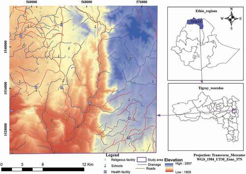
The study area is situated at the Eastern Tigray Northern Ethiopia at four different woredas located at about 57 km from Mekelle city. Geographically, the area is located in zone 37 bounded by UTM coordinates of 557,000 − 578,000 m E, and 1,525,000 − 1,546,500 m N covering a total area of 507.6 km² (Figure 1). The locality is accessed by an asphalt road running from Mekelle to Adigrat and gravel road to Negash and Wukro besides alternative small trail routes to other directions.

Figure 1. Location map of the study area.

2.2 Geology

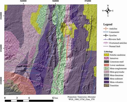
According to Gebresilassie et al. (2012), the area forms a part of the Arabian Nubian Shield and consists of Neoproterozoic low-grade N-S to NE-SW trending basement rocks of Tsaliet Group (~860 − 750 Ma) with metavolcanics, meta volcaniclastics, metasediments, and younger Tambien Group (~740 Ma) with metasediments, slate, phyllite, meta limestone, and pebbly slate (diamictite). Apart from foliation, Tambien Group rocks show development of synclinal structures (Negash syncline). These structures are intruded by post-tectonic granitoid (~600 Ma) and overlain unconformably by fluvial Paleozoic iron-rich Enticho Sandstone and Edaga Arbi Tillite and by marine Mesozoic iron-rich Adigrat sandstone, Antalo simestone, Agula shale, and Amba Aradom sandstone. Dolerite dikes also have intruded during uplift and faulting during Cenozoic time. Tsaliet metavolcanics cover the largest area (35.19%) followed by meta-greywacke (15.28%; Figure 2).

Figure 2. Geological map of Negash area.

2.3 Data

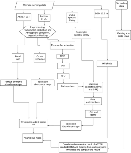
In this study, ASTER (Advanced Spaceborne Thermal Emission and Reflection Radiometer) and Landsat 8 Operational Land Imager (OLI) image data covering the suspected area of iron ore deposits in Negash were used. In this effort, VNIR and SWIR wavelengths were employed to decipher spatial distribution of iron oxide sites (Table 1). Landsat 8/Operational Land Imager images of six spectral bands (2 to 7) with a spatial resolution of 30 m were utilized in this study. Approximate scene size is 170 km north-south by 183 km east-west (106 mi by 114 mi). Secondary data including a geological map of the Wukro sheet, a topo-sheet of the Wukro area and shapefiles of different objects were supplemented. Geological survey and laboratory analysis were carried out to confirm the image processing results and iron formations prospectivity mapping them. A global positioning system (GPS) survey was also conducted in the study area for verifying the spatial distribution of alteration zones and lithological units using a handheld GPS. Additionally, numerous photos were taken from alteration zones and lithological units during the field work. Overall methodological framework and data analysis are presented in Figure 3. The remote-sensing datasets were processed using the ERDAS Imagine and ArcGIS software packages.

Table 1. Performance characteristics of satellite data.

Data set	Band name	Band width (µm)	Spatial resolution (m)	Acquisition date	Source
ASTER	1 VIS	0.52 − 0.60	15	Dec 10, 2005	http://earthexplorer.usgs.gov/
	2 VIS	0.63 − 0.69	15
	3 N NIR	0.78 − 0.86	15
	4 SWIR	1.600 − 1.700	30
	5 SWIR	2.145 − 2.185	30
	6 SWIR	2.185 − 2.225	30
	7 SWIR	2.235 − 2.285	30
	8 SWIR	2.295 − 2.365	30
	9 SWIR	2.360 − 2.430	30
Landsat 8 OLI	Band 2 – Blue	0.45 − 0.51	30	28 January 2020	https://glovis.usgs.gov/
	Band 3 – Green	0.53 − 0.59	30
	Band 4 – Red	0.64 − 0.67	30
	Band 5− Near infrared	0.85 − 0.88	30
	Band 6− SWIR 1	1.57 − 1.65	30
	Band 7− SWIR 2	2.11 − 2.29	30

Figure 3. Flowchart of the Methodology.

2.4 Data preprocessing

Preprocessing applied to ASTER imagery consisted of conversion from the DN value to radiance using radiometric calibration, layer stacking, conversion to BIL format, and atmospheric correction. For atmospheric correction, Fast Line-of-sight Atmospheric Analysis of Spectral Hypercubes (FLAASH) tropical model and rural aerosol model were adopted. On the other hand, Landsat-8/OLI DN values were converted to radiance using radiometric calibration, followed by transfer to BIL format and then applying FLAASH atmospheric correction. Tropical atmospheric conversion was followed by band match to scale reflectance between 0 and 1 and subset using study area. Finally, NDVI was calculated for both the images. Areas greater than 0.4 for ASTER and 0.3 for Landsat 8 OLI were masked as vegetation and ignored during further analysis (Tompolidi et al., 2020). The NDVI for both images was calculated from equation 1(1) $\mathrm{N}\mathrm{D}\mathrm{V}\mathrm{I}=NIR-Red/NIR+Red$(1) . Panchromatic and thermal infrared (TIR) bands, as well as bands 1, 8, and 9 of the OLI were excluded from the analysis as bands 1 and 9 are meant for coastal studies and cirrus cloud detection, respectively (Masoumi et al., 2017).

(1) $\mathrm{N}\mathrm{D}\mathrm{V}\mathrm{I}=NIR-Red/NIR+Red$(1)

where NIR is band 3 and 5, and red is band 2, and 4, for ASTER and Landsat 8 OLI, respectively.

2.5 Endmember extraction method

Endmember extraction is an important process in the creation of useful material abundance maps. Although there are different endmember extraction methods, image spectra in this study were extracted through a “spectral endmember selection” procedure, including minimum noise fraction (MNF), pixel purity index (PPI; Boardman, 1993; Boardman et al., 1995; Hosseinjani & Tangestani, 2011) and n-dimensional visualization (Boardman et al., 1995; Hosseinjani & Tangestani, 2011). An automated spectral hourglass was used to run the steps sequentially and the image endmembers were obtained at the same spatial scale as the image to be analyzed, whereas the reference endmembers were collected under different atmospheric conditions than airborne or satellite imagery and at a different spatial scale due to their proximity to objects (Adams, J.B.J.R.G.A.E. & Composition, M, 1993; Shi & Wang, 2016).

2.5.1 Pixel purity index (PPI)

First, minimum noise fraction was applied for ASTER 9 bands and 6 Landsat 8 OLI bands. Then, Pixel Purity Index (PPI) was run on the MNF data to aid in deriving endmembers from the image besides spatial data reduction. All 9 ASTER and 6 Landsat 8 OLI were used for further analysis since the eigenvalues are >1 (Hosseinjani & Tangestani, 2011). The number of iterations and thresholds used were 10,000 and 2.5 for both images.

2.5.2 N-Dimensional visualizer

The n-dimensional visualizer is an interactive tool that allows the user to select endmembers in n-space. Pixels from the spectral bands are loaded into an n-dimensional scatter plot and rotated on the visualization tool until points or extremities on the scatter plot are exposed. The ENVI n-dimensional visualizer was loaded with the top-scoring pixels from the PPI result and 10 and 7 of endmembers were retrieved from n-dimensional visualizer automatically for ASTER and Landsat 8 OLI. These endmembers were used for subsequent classification and other processing. Then, using the spectral feature fitting, the known reference spectral was matched with an unknown spectral derived from the images (Hosseinjani & Tangestani, 2011). SFF values > 0.756 were taken as endmember for ASTER image and 0.948 for Landsat 8 OLI (Kalinowski & Oliver, 2004).

2.5.3 Spectral feature fitting (SFE)

Spectral feature fitting was used to compare the fit of image spectra to reference spectra using a least-squares technique. Because SFF is an approach based on absorption features after the continuum is eliminated from both datasets, the reference spectra are scaled to match the images spectra.

2.6 Abundance mapping techniques

2.6.1 Band ratio

The band ratio is a simple and effective method for identifying and demarcating iron ore mineral occurrences (Gopinathan et al., 2020). Band ratios 6/4 (ferrous iron oxides) and 4/3 (ferric iron oxides) of Landsat 8 OLI (Cardoso-Fernandes et al., 2019) and band 2/band 1 (for Fe³⁺), 4/5 (Laterite) and band 5/band 3 + band 1/band 2 (for Fe²⁺) of ASTER were used in this study (Gopinathan et al., 2020).

2.6.2 Feature-oriented principal component selection (FPCS)

Feature-oriented main component selection or Crosta Technique is a method based on PCA (Traore et al., 2019). Only the bands of the image that have a reflection and absorption are used in feature-oriented principal component selection. The ability to forecast whether the target surface type is highlighted by dark or bright pixels in the matching principal component image is a key feature of this method. In this investigation, the Crosta approach was utilized and ASTER bands 1, 2, 3 and 4 (Traore et al., 2019) and Landsat 8 OLI bands 2, 4, 5 and 6 (Osinowo et al., 2021) were employed for iron oxide mapping.

2.6.3 Linear spectral unmixing (LSU)

The LSU is a sub-pixel image processing algorithm, which was used to determine the abundance of the minerals in each pixel of an image. The reflectance at each pixel of the image is assumed to be a linear combination of the reflectance of each material (endmember) present within the pixel. However, there are certain limitations in applying the linear spectral unmixing technique. The results of spectral unmixing are highly dependent on the input of endmembers and changing endmembers also alter the final results (Gopinathan et al., 2020). In this study, LSU was applied on the MNF images of the ASTER and Landsat 8 OLI images using different endmembers.

2.6.4 Mixture tuned matched filtering (MTMF)

MTMF improves performance over MF alone by combining components of hyperdimensional convex geometry spectral unmixing and statistically matched filter target detection. It maintains the MF’s ease of calculation while allowing for increased target selectivity, excelling at the accurate mapping of extremely small subpixel targets with low false alarm rates. When utilized on the same input data as other methods that previously had a high number of false alarms, MTMF frequently delivers low false alarm rates. This increase in performance demonstrates the effectiveness of the approach mixture tuning (MT) component. More challenging applications are needed to fully quantify the detection versus false alarm rejection. MTMF was applied for iron oxide target detection for both images using generated endmembers. Thresholding of MF score was used for target detection (Boardman & Kruse, 2011).

2.6.5 Correlation and model validation

To correlate the results obtained from remote-sensing analysis Pearson correlation coefficient was used. To operate 1000 random points were generated using 50 rows and 50 columns, then correlation was calculated from ASTER and Landsat 8 OLI. The Pearson correlation coefficient results were interpreted as strong correlation values ranging from ±0.50 to ± 1, a medium correlation is defined as ± 0.30 to ± 0.49, and a weak correlation is defined as one with a value of less than ± 0.30 (Bekele et al., 2022).

Validation of accuracy is a process that involves evaluating the accuracy of a product and becomes an integral part of any remotely sensed data-derived map. It is critical to know the maps accuracy before making any decisions based on it. The most frequent metric of map accuracy is positional accuracy, which is a measure of how closely the imagery matches with the ground truth. Although there are different accuracy assessment techniques, in this study, visual interpretation and existing iron oxide maps of the study area were digitized into polygons and overlain to the mapped results to check the positional accuracy as applied by Foody (2002).

2.6.6. Anomalous (potential) area detecting

An anomaly is a pattern in the image data that does not follow the expected behavior, also referred to as outliers, exceptions, peculiarities (Chandola et al., 2009; Zhou et al., 2016). To acquire quantitative information about the areas of mineral abundances, thresholding (or density slicing) is applied to the transformed data to separate the high potential pixels (anomalous areas) and exclude iron oxide lower concentrations as applied similarly by (Wambo et al., 2020). A threshold was applied on band ratios, selected PCA and LSU which is generated using the mean and standard deviation. The standard deviation employed varies with the confidence level used to calculate the anomaly as applied by San et al. (2004). Before calculating the threshold, the results were stretched to 0 − 255 and mean and standard deviation was taken from the basic statistics. For MTMF results 2D scatter plot was used to identify the pixels with low infeasibilities and high MF scores. MF results in the x-axis and infeasibility in the y-axis were utilized. Pixels lying in the bottom right corner were selected as potential areas since they have high MF and low infeasibility values as done by Calin et al. (2015). The threshold is calculated using equation 2(2) $Threshold=X+SD$(2) .

(2) $Threshold=X+SD$(2)

If confidence level is 92%, 2SD if 95% and 3SD if 98%, where X is mean, and SD is standard deviation.

3. Results

3.1 NDVI

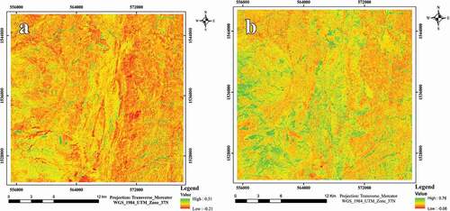
The NDVI image of Landsat 8 OLI was in the range of −0.21 to 0.51 while that derived from ASTER lied between – 0.08 and 0.76 (Figure 4a and 4b). The green portions show highly vegetated zones along stream beds and valleys in contrast to less vegetated areas of moderate yellow regions and shadow and bare lands of red patches.

Figure 4. NDVI map generated from Landsat 8 OLI (a), and ASTER (b).

3.2 Ratio maps

3.2.1 Ferrous and ferric iron

The ferrous mineral are abundance map generated from Landsat 8 OLI shows that the targets are in the Abrha-we-Atsbha area (Figure 5a). On the other hand, in ASTER map, the ore is found to be high in the Saze area mountains and west of Tsenkanet (Figure 5b). The anomalous area covered was 56.8 km² and 13.75 km² for ASTER and Landsat images, respectively. These areas were identified by a threshold value above 220 and confidence level of 92% in the case of ASTER and a threshold value of 197.2 and a confidence level of 95% in the instance of Landsat 8 OLI (Table 2).

Table 2. Threshold, confidence level and area mapped using all techniques.

Sensor	Technique	Confidence level	Threshold used	Area in (km^2)
ASTER	Band 2/1	92%	222.8	62.1
	Band 5/3 + 1/2	92%	220	56.8
	Band 4/5	92%	210	57.8
	Selective PCA	95%	210.5	34.79
	Unmixing (goethite)	92%	197	8.4
	Unmixing (hematite)	98%	185	26.5
	Goethite MF			16.4
	Hematite MF			52
Landsat 8 OLI	Band 6/4	95%	197.2	13.75
	Band 4/3	95%	188	13.2
	Selective PCA	95%	214.2	32.5
	MF (goethite)			28.4
	MF (hematite)			14.8

Figure 5. Ferrous iron anomaly map generated from Landsat 8 OLI (a), ASTER (b), and ferric iron anomaly generated from Landsat 8 OLI (c), and ASTER (d).

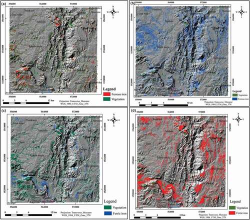
Ferric iron identified through Landsat 8 is dominant in the north around Sendeda, north of Graaras, north of Genfel and southwest around Abrha Atsbha areas (Figure 5c). Similarly, the demarks by ASTER are found in the cavity area around Adi Ksandid and other localities as Abraha Atsbha, Zarema and Graaras (Figure 5d). The said areas were mapped using a threshold value of 222.8 with 92% confidence level and a threshold value of 188 with 95% confidence level to an extent of 62.1 km² and 13.2 km², respectively for ASTER and Landsat 8 OLI (Table 2).

3.2.2 Laterite distribution

Threshold values >210 with a 92% confidence level were taken to prepare laterite distribution map using ASTER (Table 2). From Figure 6a, laterite distribution is seen dominated in the southwest and southeast. The area covered by anomaly is 57.8 km².

Figure 6. Laterite anomaly map generated from ASTER band ratio (a), anomaly map generated from PC4 Landsat 8 OLI (b), ASTER PC4 (c), and (d) final endmembers extracted from (a) ASTER, and (b) Landsat 8 OLI.

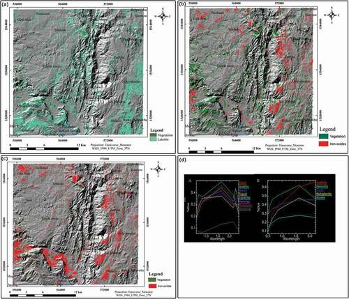
3.2.3 Selective PCA distribution

Table 3 shows strong PCA4 values −0.79 and 0.60 of opposing signs between band 1 and 2 and a low contribution of bands 3 and 4. As a result, the target areas were located around Graaras, Zarema, Adi mesanu and Abrha atsbha (Figure 6c). Similarly, Table 4 displays strong PCA4 values between 0.85 and −0.51 between bands 2 and 4 and a low contribution of bands 5 and 6. To map in bright the PCA4 was negated. As an outcome, the target areas were located around Graaras and Abrha atsbha and Sendeda, Zarema and Adi mesanu (Figure 6b).

Table 3. ASTER bands 1, 2, 3 and 4 eigenvector loadings.

Eigenvectors	Band 1	Band 2	Band 3	Band 4
PC 1	−0.332	−0.473	−0.515	−0.634
PC 2	−0.428	−0.512	−0.152	0.729
PC 3	0.267	0.39	−0.844	0.254
PC 4	0.797	−0.602	−0.013	0.042

Table 4. Landsat bands 2, 4, 5 and 6 eigenvector loadings.

Eigenvectors	Band 2	Band 4	Band 5	Band 6
PC 1	0.189	0.443	0.492	0.725
PC 2	−0.365	−0.468	−0.436	0.677
PC 3	−0.323	−0.567	0.753	−0.08
PC 4	0.853	−0.513	−0.010	0.098

3.3 End members extracted

Since the eigenvalues are >1 all 9 ASTER and 6 Landsat 8 OLI were used in the analysis (Table 5). SFF values > 0.75 were taken as endmembers for ASTER image (Table 6) and SFF values >0.95 as endmembers for Landsat 8 OLI (Table 7). Finally, 5 for Landsat 8, and 8 for ASTER endmembers were used in this study (Figure 6d). The SFF values in ASTER were 0.85 and 0.81 for hematite and goethite, respectively, whereas they were 1 for both hematite and goethite in Landsat 8 OLI (Tables 6 and 7).

Table 5. MNF eigen values of ASTER and Landsat 8 OLI.

Eigenvalues
ASTER		Landsat 8 OLI
MNF 1	57.2	MNF 1	16.1
MNF 2	29.3	MNF 2	7.8
MNF 3	11.1	MNF 3	6.4
MNF 4	8.2	MNF 4	5.8
MNF 5	6.2	MNF 5	3.4
MNF 6	5.8	MNF 6	1.99
MNF 7	3.8
MNF 8	3.3
MNF 9	2.6

Table 6. Unknown and reference spectral curve matching values of ASTER.

n-D class mean	SFF value	Matched known mineral
1	0	No matching mineral
2	0.95	Topaz
3	0.81	Goethite
4	0.96	Alunite
5	0.99	Topaz 2
6	0	No matching mineral
7	0.77	Lepidolite
8	0.85	Hematite
9	0.97	Pyrophyllite
10	0.82	Hornblende

Table 7. Unknown and reference spectral curves matching values of Landsat 8 OLI.

n-D class mean	SFF	Matched mineral
1	1	Goethite
2	1	Kaolin
3	1	Hematite
4	1	Alunite
5	0	No matching mineral
6	1	Wollastonite
7	0	No matching mineral

3.4 Linear spectral unmixing and mixture tuned matched filtering

The results of linear spectral unmixing are an abundance map for each end member and one RMS error image. The bright areas indicate a high abundance of the endmember whereas dark areas represent low abundance. The fraction image for the study site gives information about the relative abundance of the end member material considering each end member present in a pixel. The analysis of MTMF produces a collection of rule images that correlate to both the MF and infeasibility scores for each pixel when compared to each endmember spectrum (two rule images per endmember). Places with higher MF scores appear as brighter pixels in the MF images, showing areas with a large abundance of the associated endmember.

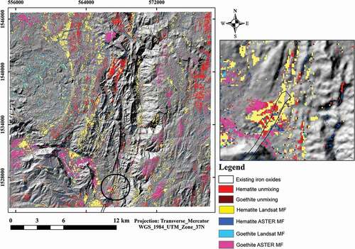
In order to map the anomalous areas from unmixing results, a threshold value of 197 with 92% confidence level for goethite and a threshold value of 188 with 98% confidence level for hematite were chosen (Table 2). In terms of the area mapped, hematite unmixing has a maximum of 26.4 km² cover whereas goethite unmixing has a least area 8.3 km². In Figures 7a and 7b, Saze area shows high goethite and hematite anomalous area. From the MTMF results of both images, the potential areas were identified based on MF scores and infeasibility images. Red and green areas in the scatter plots are abundance areas excluding false positives (Figure 7c and 7d). The areas having high MF and low infeasibility are shown in Figures 8a 8 8d.

Figure 7. ASTER unmixing (a) Goethite anomaly and (b) Hematite anomaly, and scatter plots showing high MF and low infeasibility goethite and hematite of ASTER (c), and Landsat 8 OLI (d).

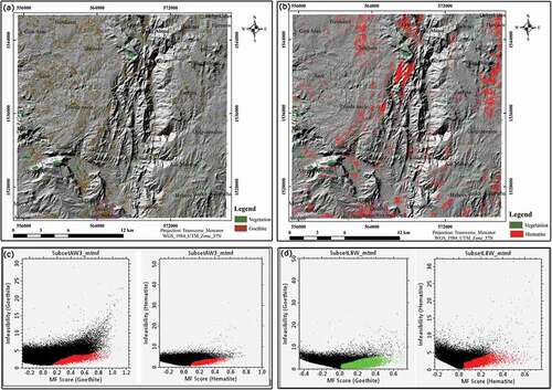
Figure 8. ASTER MTMF (a), Goethite anomaly and (b) Hematite anomaly and Landsat 8 OLI MTMF (c) Goethite anomaly and (d) Hematite anomaly.

3.5 Correlation and model validation

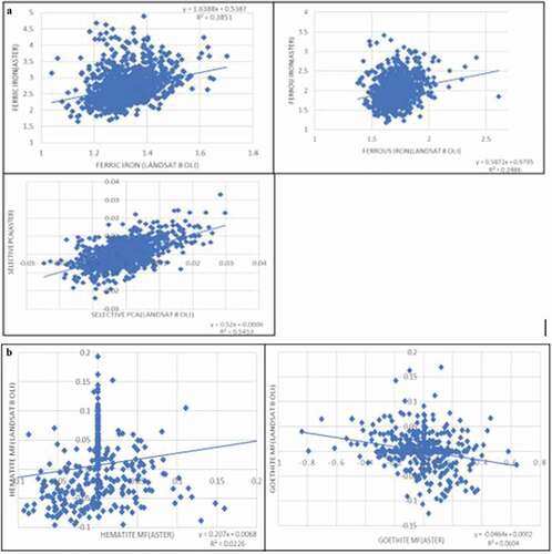
Landsat 8 OLI and ASTER for laterite results showed a high correlation (r = 0.59) in the case of selective PCA and moderate correlation (r = 0.3) for ferric iron and a poor correlation (r = 0.22) for ferrous iron. In instances of unmixing and MTMF, both hematite and goethite showed high positive (r = 0.5) and poor negative correlation (r = −0.25; Figures 9a and 9b) made similar observations.

Figure 9. Graphs showing correlation b/n results obtained from pixel-level image processing of Landsat 8 OLI and ASTER (a) and correlation b/n results obtained from Landsat OLI, and ASTER MTMF (b).

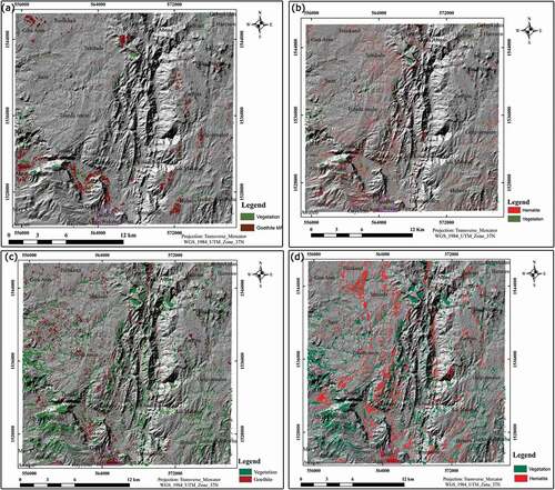
The ASTER results portray that the existing iron oxide polygons overlay with the iron oxides of ferric iron, laterite, and ferrous iron, but the band ratio obtained from Landsat 8 OLI was poor (Figure 10a). Figure 10b obtained from selective PCA depicts a better overlay with in the existing iron oxide polygons. Although, both overlays point out similar results, selective PCA of ASTER fits better than the other (Landsat 8 OLI). However, Figure 11 indicates that results obtained from unmixing and MTMF overlays fits better than the latter (ASTER). The results obtained from MF ASTER has a better fit with the existing polygons.

Figure 10. Ratio of anomalous areas overlay on polygons of the existing iron oxides (a), and selective PCA results overlay with existing iron oxide polygons (b).

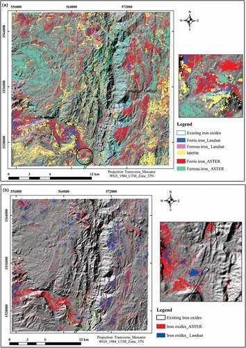
Figure 11. Unmixing and MTMF results overlay on existing iron oxide polygons.

4 Discussion

The comparative superior spectral and spatial characteristics of ASTER and Landsat 8 OLI images provide useful information on the delineation of iron ore deposits. In the wavelength ranges covered by Landsat TM bands 1 (blue) and 2 (green), which are analogous to bands 2 (blue) and 3 (green) in Landsat 8 OLI, vegetation and iron oxides show similar reflectance spectra. In places with heavy or low vegetation cover, these bands are not very useful for differentiating iron oxides. In order to overcome this interference while mapping the iron ore bands, first vegetation was masked out during the present investigation. So, initially different vegetation indices such as ratio indices and soil adjusted vegetation indices and NDVI were mapped. In this method, since NDVI saturates above 0.7 values, the maps were convenient in finding areas that contain either the country rocks or the iron ore bands. This procedure was also adopted by Gopinathan et al. (2020) during mapping of iron oxides in Tamil Nadu. The use of masking to remove vegetation interference helped to delineate the areas with high iron oxide content of values greater than 0.3 for Landsat 8 OLI and 0.4 for ASTER. A similar technique was employed by Tompolidi et al. (2020) for mapping hydrothermal field in volcanic environment in Greece. Vegetation masking in ASTER images was denser than that in Landsat 8 OLI images and these observations are in agreement with the findings of Traore et al. (2019).

Band ratio techniques were used to generate the abundance of iron oxide content in various parts of the study area. Each object has its own spectral reflectance pattern in different wavelength regions. The object or a rock unit may have high reflectance value in some spectral regions, though it may be absorbed in other spectral regions. For instance, iron ore absorbs electromagnetic radiation (EMR) in the 0.85–0.9 μm region. In this context, the band ratios serve as a simple and powerful tool to identify and demarcate the iron ore mineral deposits. As consequence, the results were obtained in different band ratios such as band 2 and 1 for Ferric (Fe³⁺), for band 5 and 3 + band 1 and 2 for Ferrous iron (Fe²⁺), and band 4 and 5 for laterite in ASTER and in band 6 and 4 for Ferrous (Fe²⁺), band 4 and 3 for ferric iron (Fe³⁺) in Landsat 8 OLI. Although band 4 and 2 were also tested to map ferric iron from Landsat 8 OLI image(s), the out put was very poor. To distinguish the minerals, threshold value for each resultant image was computed statistically by way of mean and standard deviation, as followed similarly by San et al. (2004) during his work on comparison of band ratioing and spectral indices methods for detecting alunite and kaolinite minerals using ASTER data in Biga region, Turkey. The values above the threshold were overlain on the hill shade images of ASTER and Landsat 8 OLI. The high anomalous iron content in the western part of the study area in the ferrous iron map and laterite map generated from ASTER could be explained by the alteration of biotite in granite to iron oxides as interpreted by Cardoso-Fernandes et al. (2019).

Different bands in multispectral data were often highly correlated and contained similar information. To map iron oxides, four bands were chosen from each ASTER and Landsat 8 OLI images. The bands were selected based on absorptive and reflective characteristics of the mineral of interest. As given in Table 4, PCA 4 showed strong values (0.853 and −0.513) of opposing signs between bands 2 and 4, but low contribution from bands 5 and 6. Similarly, in Table 3, PCA 4 showed strong values (−0.79 and 0.60) of opposing signs between band 1 and 2, but low contribution from bands 3 and 4. From both images, PCA 4 was selected since the values were high with opposite magnitude for PCA 4, of ASTER in bands 1 and 2 and in Landsat 8 in bands 2 and 4. Negative values in reflective bands indicate that iron oxides are dark. But to show them in bright, the PCA 4 was multiplied by −1, as done by Traore et al. (2019). And the target was sliced using 210.5 and 214.2 thresholds for ASTER and Landsat 8 OLI, respectively to map anomalous areas.

In this study, minimum noise fraction was applied for 9 bands of ASTER and 6 bands of Landsat 8 OLI for spectral data reduction before extracting the endmembers. All 9 ASTER and 6 Landsat 8 OLI were used for further analysis since the eigenvalues were >1. The pixel purity index (PPI) was run on the MNF data to aid in deriving endmembers from the image and to achieve spatial data reduction. The number of iterations and thresholds used were 10,000 and 2.5 for both images as applied similarly by Hosseinjani and Tangestani (2011). SFF values >0.75 were taken as endmember for ASTER image and 1 for Landsat 8 OLI and this is greater than the threshold value of 0.5 selected by (Kalinowski & Oliver, 2004). As a sequel, five endmembers for Landsat 8 and eight endmembers for ASTER were used in this work. The SFF values were 0.85 and 0.81 for ASTER and 1 for Landsat 8. Spectral unmixing results are highly dependent on the input endmembers and changing the endmembers would alter the results and this fact was proved by Gopinathan et al. (2020).

Linear spectral unmixing determines the relative abundances of materials depicted by multispectral imagery based on material spectral characteristics. The bright areas indicate a high abundance of the endmember whereas dark areas represent low abundance. Although the unmixing result was constrained to 1, the output contained a negative value, which is physically meaningless. Such negative values are the background noises that were obtained by Calin et al. (2015). Both goethite anomaly derived from ASTER unmixing as well as from Landsat 8 OLI MTMF showed high targets in the western part of the study area and could be explained by the alteration of biotite in granite to iron oxides as interpreted by Cardoso-Fernandes et al. (2019).

The MF images project areas with higher MF scores as brighter pixels, thus highlighting the areas with a large abundance of respective endmember. Perfectly mapped pixels have an MF score above the background distribution, which has some noise-limited spread around zero, and a low infeasibility value. To map the potential areas, a 2-D scatter plot was prepared using MF score and infeasibility. Pixels at the right bottom show high MF scores and low infeasibility depicting potential areas. MTMF is not dependent on the input endmembers. Although it was constrained to 1, with a negative notation that is physically meaningless, the same was interpreted by Calin et al. (2015) as background noise.

A strong correlation was obtained (r = 0.59) between the Landsat 8 OLI and ASTER results selective PCA for laterite, moderate correlation (r = 0.3) for ferric iron and a poor correlation for ferrous iron (r = 0.22). For unmixing and MTMF results, both hematite and goethite have a poor positive and negative correlation with an r each of 0.15 and −0.25 respectively which was similarly interpreted by Bekele et al. (2022) for LST. While validating the results obtained through selective PCA, the best fit was obtained for the existing iron oxide polygons and the band ratio showing a poor match in Landsat 8 OLI image. The results obtained from hematite unmixing and goethite ASTER MTMF have a better fit with the existing polygons whereas hematite ASTER MF showed a good overlay. The MTMF obtained from Landsat 8 OLI and goethite unmixing showed a very poor overlay. The comparison thus shows that ASTER mapped better than Landsat 8 OLI for band ratios, selective PCA, unmixing and MTMF.

Conclusion

The geo-spatial techniques used to identify, map and demarcate the iron ore deposits in the present instance could profitably be made use of to locate several other mineral resources in the country. The method employed is an advanced technique that takes little time, modest money and tiny effort to characterize and map large resources effectively in a country like Ethiopia with many constraints.

Acknowledgments

We are thankful to the School of Earth Sciences, Addis Ababa University, for providing facilities, and funds. Mr. Haylemikeal grateful to Mekelle University to sponsor for his higher studies in Remote-sensing and Geo-informatics. We are also gratefully acknowledge two anonymous reviewers and Dr. Daren Jones, Associate Editor for their critical and constructive comments of the manuscript.

Disclosure statement

No potential conflict of interest was reported by the author(s).

References

- Aboelkhair, H., Ninomiya, Y., Watanabe, Y., & Sato, I. (2011). Processing and interpretation of ASTER TIR data for mapping of rare-metal-enriched albite granitoids in the central eastern desert of Egypt. Journal of African Earth Sciences, 58,141–151.
- Adams, J.B.J.R.G.A.E., & Composition, M. (1993). Imaging spectroscopy: (pp. 145–166). Interpretation based on spectral mixture analysis.
- Azizi, M., & Saibi, H. (2015). Integrating gravity data with remotely sensed data for structural investigation of the Aynak-Logar Valley, eastern Afghanistan, and the surrounding area. IEEE J. Selected Top. IEEE Journal of Selected Topics in Applied Earth Observations and Remote Sensing, 8(2), 816–824. https://doi.org/10.1109/JSTARS.2014.2347375
- Azizi, M., Saibi, H., & Cooper, G. R. J. (2015). Mineral and structural mapping of the Aynak-Logar Valley (Eastern Afghanistan) from hyperspectral remote sensing data and aeromagnetic data. Arabian Journal of Geosciences, 8(12), 10911–10918. https://doi.org/10.1007/s12517-015-1993-2
- Azizi, H., Tarverdi, M. A., & Akbarpour, A. (2010). Extraction of hydrothermal alterations from ASTER SWIR data from east Zanjan, northern Iran. Advances in Space Research, 46(1), 99–109. https://doi.org/10.1016/j.asr.2010.03.014
- Bedini, E. (2011). Mineral mapping in the kap simpson complex, central East Greenland, using HyMap and ASTER remote sensing data. Advances in Space Research, 47(1),60–73. https://doi.org/10.1016/j.asr.2010.08.021
- Bekele, N. K., Hailu, B. T., & Suryabhagavan, K. V. (2022). Spatial patterns of urban blue-green landscapes on land surface temperature: A case of Addis Ababa, Ethiopia. Current Research in Environmental Sustainability, 4,100146. https://doi.org/10.1016/j.crsust.2022.100146
- Bersi, M., Saibi, H., & Chabou, M. C. (2016). Aerogravity and remote sensing observations of an iron deposit in Gara Djebilet, southwestern Algeria. Journal of African Earth Sciences, 116,134–150. https://doi.org/10.1016/j.jafrearsci.2016.01.004
- Boardman, J. W. (1993). Automated spectral unmixing of AVIRIS data using convex geometry concepts, in Proc. Summ. 4th JPL Airborne Geosci. Workshop, vol 1, 1114, , vol 1, 1114, JPL Publication 93−26.
- Boardman, J. W., & Kruse, F. A. (2011). Analysis of imaging spectrometer data using $N$-Dimensional geometry and a mixture-tuned matched filtering approach. IEEE Transactions on Geoscience and Remote Sensing, 49(11), 4138–4152. https://doi.org/10.1109/TGRS.2011.2161585
- Boardman, J. W., Kruse, F. A., & Green, R. O. (1995). Mapping target signatures via partial unmixing of AVIRIS data, in Proc. Summ. 5th Annu. JPL Airborne Earth Sci. Workshop, 23–26.
- Calin, M. A., Coman, T., Parasca, S. V., Bercaru, N., Savastru, R. S., & Manea, D. (2015). Hyperspectral imaging-based wound analysis using mixture-tuned matched filtering classification method. Journal of Biomedical Optics, 20(4), 046004. https://doi.org/10.1117/1.JBO.20.4.046004
- Cardoso-Fernandes, J., Teodoro, A. C., & Lima, A. (2019). Remote sensing data in lithium (Li) exploration: A new approach for the detection of Li-bearing pegmatites. International Journal of Applied Earth Observation and Geoinformation, 76, 10–25. https://doi.org/10.1016/j.jag.2018.11.001
- Chandola, V., Banerjee, A., & Kumar, V. (2009). Anomaly detection: A survey. ACM Computing Surveys (CSUR), 41(3), 1–58. https://doi.org/10.1145/1541880.1541882
- Chen, X., Mao, J., & Tian, H. J. S. (2020). Analysis of China’s iron trade Flow: Quantity, value and regional pattern. Sustainability, 12(24), 10427. https://doi.org/10.3390/su122410427
- Clark, R. N., & Roush, T. L. (1984). Reflectance spectroscopy: Quantitative analysis techniques for remote sensing applications. Journal of Geophysical Research, 89, 6329–6340.
- Clark, R. N., Swayze, G. A., Heidebrecht, K., Green, R. O., & Goetz, A. F. H. (1995). Calibration to surface reflectance of terrestrial imaging spectrometry data: Comparison of methods: Summaries of the fifth annual JPL airborne Earth science workshop. JPL Publication.
- Cloutis, E. A. (1996). Review article hyperspectral geological remote sensing: Evaluation of analytical techniques. International Journal of Remote Sensing, 17(12), 2215–2242. https://doi.org/10.1080/01431169608948770
- de Morais, M. C., Martins, P. P., Júnior, & Paradella, W. R. Multi-scale approach using remote sensing images to characterize the iron deposit N1 influence areas in Carajás Mineral Province (Brazilian Amazon). (2012). Environmental Earth Sciences, 66(7), 2085–2096. 2012. https://doi.org/10.1007/s12665-011-1434-9
- Elsayed, Z. K. A., El-Nadi, A. H. H., & Babiker, I. S. (2020). Prospecting for gold mineralization with the use of remote sensing and GIS technology in North Kordofan State, central Sudan. Scientific African, 10, e00627. https://doi.org/10.1016/j.sciaf.2020.e00627
- El Zalaky, M. A., Essam, M. E., & El Arefy, R. A. (2018). Assessment of band ratios and feature-oriented principal component selection (FPCS) techniques for iron oxides mapping with relation to radioactivity using landsat 8 at Bahariya Oasis. Egypt Res, 10(4), 1–10. https://doi.org/10.7537/marsrsj100418.01
- EMD. (2011). (Ezana mining development), Mineral resource estimate and technical report on iron deposit of ShireMentebteb area, Northwestern of Tigray region, Ethiopia.
- Fakhari, S., Jafarirad, A., Afzal, P., & Lotfi, M. (2019). Delineation of hydrothermal alteration zones for porphyrysystems utilizing ASTER data in Jebal-Barez area, SE Iran. Iranian Journal of Earth Sciences, 11(1), 80–92. https://doi.org/10.30495/ijes.2019.664780
- Fantaye, A. (2009). Mapping hydrothermally altered rocks and lineament analysis through digital enhancement of aster data case study: Kemashi area. Addis Ababa University.
- Foody, G. M. (2002). The role of soft classification techniques in the refinement of estimates of ground control point location. Photogrammetric Engineering and Remote Sensing, 68(9), 897–904. http://eprints.soton.ac.uk/id/eprint/14895
- Gad, S., & Kusky, T. (2006). Lithological mapping in the Eastern Desert of Egypt, the Barramiya area, using Landsat thematic mapper (TM). Journal of African Earth Sciences, 44(2), 196–202. https://doi.org/10.1016/j.jafrearsci.2005.10.014
- Gad, S., & Kusky, T. (2007). ASTER spectral ratioing for lithological mapping in the Arabian–Nubian shield, the Neoproterozoic Wadi Kid area, Sinai, Egypt. Gondwana Research, 11(3), 326–335. https://doi.org/10.1016/j.gr.2006.02.010
- Galvao, L. S., Formaggio, A. R., & Tisot, D. A. (2005). Discrimination of sugarcane varieties in Southeastern Brazil with EO-1 Hyperion data. Remote Sensing of Environment, 94(4), 523–534. https://doi.org/10.1016/j.rse.2004.11.012
- Gebresilassie, S., Bheemalingeswara, K., & Fiseha, A. (2012). Geology and characteristics of meta-limestone-hosted iron deposit near Negash, Tigray and northern Ethiopia. International Journal of Earth Sciences and Engineering, 5(6), 1535–1544.
- Gopinathan, P., Parthiban, S., Magendran, T., Al-Quraishi, A. M. F., Singh, A. K., & Singh, P. K. (2020). Mapping of ferric (Fe3+) and ferrous (Fe2+) iron oxides distribution using band ratio techniques with ASTER data and geochemistry of Kanjamalai and Godumalai. Tamil Nadu, South India, 18, 100306. https://doi.org/10.1016/j.rsase.2020.100306
- Govil, H., Gill, N., Rajendran, S., Santosh, M., & Kumar, S. (2018). Identification of new base metal mineralization in Kumaon Himalaya, India, using hyperspectral remote sensing and hydrothermal alteration. Ore Geology Reviews, 92, 271–283. https://doi.org/10.1016/j.oregeorev.2017.11.023
- Guha, A., Kumar, K. V., Rao, E. N. D., & Parveen, R. (2014). An image processing approach for converging ASTER-derived spectral maps for mapping Kolhan limestone, Jharkhand, India. Current Science, 106(1), 2–11. https://doi.org/10.18520/CS/V106/I1/40-49
- Guha, A., Singh, V. K., Parveen, R., Kumar, K. V., Jeyaseelan, A. T., & Dhanamjaya Rao, E. N. (2013). Analysis of ASTER data for mapping bauxite rich pockets within high altitude lateritic bauxite, Jharkhand, India. International Journal of Applied Earth Observation and Geoinformation: ITC Journal, 21,184–194. https://doi.org/10.1016/j.jag.2012.08.003
- Guha, A., Yamaguchi, Y., Chatterjee, S., Rani, K., & Vinod Kumar, K. (2019). Emittance spectroscopy and broadband thermal remote sensing applied to phosphorite and its utility in geoexploration: A study in the parts of Rajasthan, India. Remote Sensing, 11(9), 1003. https://doi.org/10.3390/rs11091003
- Haldar, S. K. (2018). Mineral exploration: Principles and applications. Elsevier. https://doi.org/10.1016/C2017-0-00902-3
- Hewson, R. D., Cudahy, T. J., Mizuhiko, S., Ueda, K., & Mauger, A. J. (2005). Seamless geological map generation using ASTER in the Broken Hill-Curnamona province of Australia. Remote Sensing of Environment, 99(1-2),159–172. https://doi.org/10.1016/j.rse.2005.04.025
- Hosseinjani, M., & Tangestani, M. H. (2011). Mapping alteration minerals using sub-pixel unmixing of ASTER data in the Sarduiyeh area, SE Kerman, Iran. International Journal of Digital Earth, 4(6), 487–504. https://doi.org/10.1080/17538947.2010.550937
- Kalinowski, A., & Oliver, S. (2004). ASTER mineral index processing manual. Remote Sensing Applications. Geoscience Australia, 37, 1–36.
- Kaufmann, H., Segl, K., Guanter, L., Chabrillat, S., Hofer, S., Bach, H., Hostert, P., Müller, A., & Chlebek, C. (2009). Review of EnMAP scientific potential and preparation phase. 6th EARSeL SIG IS Workshop.
- Kumar, C., Chatterjee, S., Oommen, T., & Guha, A. (2020). Automated lithological mapping by integrating spectral enhancement techniques and machine learning algorithms using AVIRIS-NG hyperspectral data in Gold-bearing granite-greenstone rocks in Hutti, India. International Journal of Applied Earth Observation and Geoinformation, 86, 102006. https://doi.org/10.1016/j.jag.2019.102006
- Magendrana, T., & Sanjeevi, S. (2014). Hyperion image analysis and linear spectral unmixing to evaluate the grades of iron ores in parts of Noamundi, Eastern India. International Journal of Applied Earth Observation and Geoinformation, 26, 413–426. https://doi.org/10.1016/j.jag.2013.09.004
- Mars, J. C., & Rowan, L. C. (2010). Spectral assessment of new ASTER SWIR surface reflectance data products for spectroscopic mapping of rocks and minerals. Remote Sensing of Environment, 114(9),2011–2025. https://doi.org/10.1016/j.rse.2010.04.008
- Masoumi, F., Eslamkish, T., Honarmand, M., & Abkar, A. A. (2017). A comparative study of Landsat‐7 and Landsat‐8 data using image processing methods for hydrothermal alteration mapping. Resource Geology, 67(1), 72–88. https://doi.org/10.1111/rge.12117
- Mogren, S., Saibi, H., Mukhopadhyay, M., Gottsmann, J., & Ibrahim, E. (2017). Analyze the spatial distribution of lava flows in Al-Ays Volcanic Area, Saudi Arabia, using remote sensing. Arabian Journal of Geosciences, 10(6), 133. https://doi.org/10.1007/s12517-017-2889-0
- Mohamed, M. T. A., Al-Naimi, L. S., Mgbeojedo, T. I., & Agoha, C. C. (2021). Geological mapping and mineral prospectivity using remote sensing and GIS in parts of Hamissana, Northeast Sudan. Journal of Petroleum Exploration and Production Technology, 11(3), 1123–1138. https://doi.org/10.1007/s13202-021-01115-3
- Nabilou, M., Arian, M., Afzal, P., Adib, A., & Kazemi, A. (2018). Determination of relationship between basement faults and alteration zones in Bafq-Esfordi region, central Iran. Episodes Journal of International Geoscienc, 41(3), 143–159. https://doi.org/10.18814/epiiugs/2018/018013
- Ni, L., Xu, H., & Zhou, X. (2020). Mineral identification and mapping by synthesis of Hyperspectral VNIR/SWIR and Multispectral TIR remotely sensed data with different classifiers, in IEEE. Journal of Selected Topics in Applied Earth Observations and Remote Sensing, 13, 3155–3163. https://doi.org/10.1109/JSTARS.2020.2999057
- Omer, E. A. H., & Elsayed Zeinelabdein, K. A. (2018). Digital image processing of Landsat 8 and spectral analysis of ASTER data for mapping alteration minerals, Southern Hamisana, NE Sudan. Al Neelain. Journal of Geosciences, 2(1), 10–20. http://hdl.handle.net/123456789/13555.
- Osinowo, O. O., Gomy, A., & Isseini, M. (2021). Mapping hydrothermal alteration mineral deposits from Landsat 8 satellite data in Pala, Mayo Kebbi Region, Southwestern Chad. Scientific African, 11, e00687. https://doi.org/10.1016/j.sciaf.2020.e00687
- Pal, S. K., Majumdar, T. J., Bhattacharya, A. K., & Bhattacharyya, R. (2011). Utilization of Landsat ETM+ data for mineral-occurrences mapping over Dalma and Dhanjori, Jharkhand, India: An advanced spectral analysis approach. International Journal of Remote Sensing, 32(14), 4023–4040. https://doi.org/10.1080/01431161.2010.484430
- Pour, A. B., & Hashim, M. (2012). The application of ASTER remote sensing data to porphyry copper and epithermal gold deposits. Ore Geology Reviews, 44, 1–9. https://doi.org/10.1016/j.oregeorev.2011.09.009
- Pour, A. B., Hashim, M., Hong, J. K., & Park, Y. (2019). Lithological and alteration mineral mapping in poorly exposed lithologies using Landsat-8 and ASTER satellite data: North-eastern Graham Land, Antarctic Peninsula, Ore Geology Reviews, 108, 112–133. http://dx.doi.org/10.1016/j.oregeorev.2017.07.018
- Pour, A. B., Hashim, M., & Marghany, M. (2011). Using spectral mapping techniques on short wave infrared bands of ASTER remote sensing data for alteration mineral mapping in SE Iran. International Journal of the Physical Sciences, 6(4), 917–929. https://doi.org/10.5897/IJPS10.510
- Pour, A. B., Hashim, M., Park, Y., & Hong, J. K. (2018). Mapping alteration mineral zones and lithological units in Antarctic regions using spectral bands of ASTER remote sensing data. Geocarto International, 33(12), 1281–1306. https://doi.org/10.1080/10106049.2017.1347207
- Qiu, F., Abdelsalam, M., & Thakkar, P. (2006). Spectral analysis of ASTER data covering part of the Neoproterozoic Allaqi-Heiani suture, Southern Egypt. Journal of African Earth Sciences, 44(2), 169–180. https://doi.org/10.1016/j.jafrearsci.2005.10.009
- Rajendran, S., Al-Khirbash, S., Pracejus, B., Nasir, S., Al-Abri, A. H., Kusky, T. M., & Ghulam, A. (2012). ASTER detection of chromite bearing mineralized zones in Semail Ophiolite Massifs of the northern Oman Mountains: Exploration strategy. Ore Geology Reviews, 44, 121–135. https://doi.org/10.1016/j.oregeorev.2011.09.010
- Rajendran, S., Nasir, S., Kusky, T. M., Ghulam, A., Gabr, S., & El-Ghali, M. A. (2013). Detection of hydrothermal mineralized zones associated with listwaenites in Central Oman using ASTER data. Ore Geology Reviews, 53, 470–488. https://doi.org/10.1016/j.oregeorev.2013.02.008
- Ranjbar, H., Honarmand, M., & Moezifar, Z. (2004). Application of the Crosta technique for porphyry copper alteration mapping, using ETM+ data in the southern part of the Iranian volcanic sedimentary belt. Journal of Asian Earth Sciences, 24(2), 237–243. https://doi.org/10.1016/j.jseaes.2003.11.001
- Saadi, N., Aboud, E., Saibi, H., & Watanabe, K. (2008a). Integrating data from remote sensing, geology and gravity for geological investigation in the Tarhunah area, northwest Libya. International Journal of Digital Earth, 1(4), 347–366. https://doi.org/10.1080/17538940802435844
- Saadi, N., Watanabe, K., Imai, A., & Saibi, H. (2008b). Integrating potential fields with remote sensing data for geological investigations in the Eljufra area of Libya. Earth, Planets and Space, 60(6), 539–547. https://doi.org/10.1186/BF03353116
- Saed, S., Azizi, H., Daneshvar, N., Peyman Afzal, P., Whattam, S. A., & Mohammad, Y. O. (2022). Hydrothermal alteration mapping using ASTER data, Takab-Baneh area, NW Iran: A key for further exploration of polymetal deposits. Geocarto International. https://doi.org/10.1080/10106049.2022.2059110
- Saibi, H., Bersi, M., Mia, M. B., Saadi, N. M., Al Bloushi, K. M. S., & Akavian, R. W. (2018). Applications of remote sensing in Geosciences. In M.-C. Hung & Y.-H. Wu (Eds.), Recent Advances and Applications in Remote Sensing Book, Intech Edition (pp. 181–203). (Chapter 9).
- San, B. T., Sumer, E. O., & Gurcay, B. (2004). Comparison of band ratioing and spectral indices methods for detecting alunite and kaolinite minerals using ASTER data in Biga region, Turkey. In Proceedings ISPRS.
- Schubert, G. (2015). Treatise on geophysics. Elsevier.
- Settle, J. J. (2006). On the effect of variable endmember spectra in the linear mixture model, IEEE. IEEE Transactions on Geoscience and Remote Sensing, 44(2), 389–396. https://doi.org/10.1109/TGRS.2005.860983
- Shaik, I., Begum, S. K., Nagamani, P. V., & Kayet, N. (2021). Characterization and mapping of hematite ore mineral classes using hyperspectral remote sensing technique: A case study from Bailadila iron ore mining region. SN Applied Sciences, 3(2), 182. https://doi.org/10.1007/s42452-021-04213-3
- Shi, C., & Wang, L. (2014). Incorporating spatial information in spectral unmixing: A review. Remote Sensing of Environment, 149, 70–87. https://doi.org/10.1016/j.rse.2014.03.034
- Shi, C., & Wang, L. (2016). Linear Spatial Spectral Mixture Model. IEEE Transactions on Geoscience and Remote Sensing, 54(6), 1–13. https://doi.org/10.1109/TGRS.2016.2520399
- Tadesse, S. (2009). Mineral resources potential of Ethiopia. Addis Ababa University Press.
- Tompolidi, A.-M., Sykioti, O., Koutroumbas, K., & Parcharidis, I. (2020). Spectral unmixing for mapping a hydrothermal field in a volcanic environment applied on ASTER, Landsat-8/OLI, and Sentinel-2 MSI satellite multispectral data: The Nisyros (Greece) case study. Remote Sensing, 12(24), 4180. https://doi.org/10.3390/rs12244180
- Transon, J. D., Andrimont, R., Maugnard, A., & Defourny, P. (2018). Survey of hyperspectral earth observation applications from space in the sentinel-2 context. Remote Sensing, 10(3), 157. https://doi.org/10.3390/rs10020157
- Traore, M., Çan, T., & Tekin, S. (2019). Discrimination of iron deposits using feature-oriented principal component selection and band ratio methods: Eastern Taurus/Turkey. International Symposium on Applied Geoinformatics, ISAG2019 was held in Istanbul on, 9.
- Van der Meer, F. D., Van der Werff, H. M., Van Ruitenbeek, F. J., Hecker, C. A., Bakker, W. H., Noomen, M. F., Van Der Meijde, M., Carranza, E. J. M., De Smeth, J. B., & Woldai, T. (2012). Multi-and hyperspectral geologic remote sensing: A review. International Journal of Applied Earth Observation and Geoinformation, 14(1), 112–128. https://doi.org/10.1016/j.jag.2011.08.002
- Wambo, J. D. T., Pour, A. B., Ganno, S., Asimow, P. D., Zoheir, B., Dos Reis Salles, R., Nzenti, J. P., Pradhan, B., & Muslim, A. M. (2020). Identifying high potential zones of gold mineralization in a sub-tropical region using Landsat-8 and ASTER remote sensing data: A case study of the Ngoura-Colomines goldfield, eastern Cameroon. Ore Geology Reviews, 122, 103530. https://doi.org/10.1016/j.oregeorev.2020.103530
- Winter, M. E. (2000). Comparison of approaches for determining end-members in hyperspectral data. IEEE Aerospace Conference. Proceedings (Cat. No. 00TH8484): IEEE, 305–313.
- Yazdi, Z., Rad, J. A., Aghazadeh, M., & Afzal, P. (2018). Alteration mapping for porphyry copper exploration using ASTERand QuickBird multispectral images, sonajeel prospect, NW Iran. Journal of the Indian Society of Remote Sensing, 46(10), 1581–1593. https://doi.org/10.1007/s12524-018-0811-1
- Zamyad, M., Afzal, P., Pourkermani, M., Nouri, R., & Jafari, M. R. (2019). Determination of hydrothermal alteration zones using remote sensing methods in Tirka area, Toroud, NE Iran. J Indian Soc Rem. Sens.Arab. J. Geosci.IEEE J. Selected Top. Appl. Earth Observ. Arabian Journal of Geosciences, 47, 1817–1830. https://doi.org/10.1007/s12524-019-01032-3
- Zhou, Z. G., Tang, P., & Zhou, M. (2016). Detecting anomaly regions in satellite image time series based on seasonal autocorrelation analysis. ISPRS Annals of the Photogrammetry. Remote Sensing and Spatial Information Sciences, 3, 303. https://doi.org/10.5194/isprs-annals-III-3-303-2016