An empirical model of the decision to switch between electricity price contracts

ABSTRACT

In this paper, we explore how sensitive the timing of switches between electricity contracts is to current and past prices. We present a model for time series of individual binary decisions which depends on the history of past and present prices. The model is based on the Bayesian learning procedure which is at the core of sequential decision-making. Given a-priori distributions of the information conditional on the state of the world, we show that the model captures dependence on past prices in a straightforward fashion. We estimate by maximum likelihood the parameters of the model on a sample of Swedish households who decide over time between competing electricity price contracts. The estimated parameters suggest that households do respond to prices by switching between contracts and that the response to price can be sizeable for alternative price processes. Importantly, the model structure implies that in general, the response to a price change will not be immediate but delayed.

KEYWORDS:

• Binary decision
• Bayesian learning
• contract choice
• price
• survival analysis

1. Introduction

Households repeatedly face the decision to switch between many different types of contracts and tariffs, including electricity pricing contracts (hereinafter referred to as electricity contracts) (Goett, Hudson, & Train, 2000; Juliusson, Gamble, & Garling, 2007), internet services (Lambrecht, Seim, & Skiera, 2007), telephone services (Braun & Schweidel, 2011; Miravete, 2002; Miravete & Palacios-Huerta, 2014) and mortgage rates (Dhillon, Shilling, & Sirmans, 1987). Analysing these choices is important from an economic perspective as it provides insights into the precise nature of the household’s decision-making, how they process the information available to them and how their decision depends on their current economic situation. The financial implications of the choices are important for retailers (Gupta et al., 2006; Lambrecht & Skiera, 2006) and the optimal regulation of such markets rests on the results from analyses of this kind (Brennan, 2007). This is true in particular for the case of electricity contracts, which is the topic of the current paper.

Figure 9. Average survival function, price information only, homoscedastic specification.

The figure shows the average (over 250 possible histories of the variable price) survival function (survival with a variable-price contract) for different fixed prices based on the model specification which includes price information only and allows for information discounting.

The choice of electricity contract is one of the many margins of choice the household face (together with choice of retailer, energy efficiency, etc.), and may be a non-negligible aspect of electricity demand price responsiveness. From a policy perspective, it is therefore important to understand this choice in order to regulate electricity pricing effectively (e.g., Defeuilley, 2009; Ek & Söderholm, 2008; Littlechild, 2006). For example, active consumers who switch between contracts in response to prices may reduce the scope for retailers to exercise market power (Goett et al., 2000). Finally, understanding how households choose between electricity contracts is also of importance to retailers and their pricing policies. Given the alternative prices, the value to the retailer of a specific contract will depend how long the household remains with that contract.

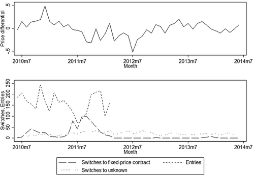
Understanding this choice involves many complicating factors. First, from the households’ point of view, determining which type of contract is the most beneficial is a difficult exercise since the future prices are unknown and previous prices may for some periods be similar across contracts and for other periods very different (for example, see the upper panel of Figure 1). Second, the household may need to be convinced by observable facts before she agrees to change her mind about her current contract. Hence, it is plausible that households respond to the history of past prices, rather than the last price only. In our data, switches between contracts typically do not occur immediately after large price shocks, but rather few months later; Figure 1 illustrates this fact for the data used in this paper. The fact that households face different price histories depending on, for example, when they signed their contract, could then explain why some households, in a given month, switch contract while others don’t. The dependence of the decision on the history of past prices may also explain why households abstain from switching between contracts, even if the evidence of recent prices appears to favour frequent switching.

Figure 1. Number of Swedish households on each type of contract and price per kWh.

One SEK is roughly 0.1 Euro. Fixed-price contract refers to contracts with prices fixed for a year or longer (typically up to three years), and variable-price contract refers to contracts with prices varying by month. See footnote 1 for other type of contracts available to Swedish households. In addition to the price per kWh, households pay for transmission, green certificate and taxes. These costs (which are not included in the figure above) amounts to roughly 0.5 SEK/kWh, plus a fixed annual transmission fee varying between 1500 and 15000 SEK depending on the required amperage. These additional costs are identical for both type of contracts. The two vertical lines at June 2010 and February 2012 represents the time period during which households in the sample start their variable-price contract, as explained in Section 3. The households in the sample are then followed over time until June 2014.

The previous literature on determinants of electricity contract choice is limited, and in many cases, the analysis relies on the stated preference approach where the effect of prices is difficult to measure. Goett et al. (2000) explore the willingness-to-pay for electricity contract attributes, and find that households are willing to pay a small premium ($0.008$ USD per kWh) to avoid seasonal price variability. Juliusson et al. (2007) explore how loss aversion and beliefs about future prices affect the probability to select a contract with prices varying across months, and find a negative effect for both. However, the author is unable to describe in more detail how these beliefs are formed, and how they depend on, e.g., previous prices. Schleich, Faure, and Gassmann (2019) explores contract switching (and retailer switching) using survey data from eight EU countries and finds that determinants of contract switching includes potential financial benefits, environmental preferences and income. Vesterberg (2018) is one of the few previous papers that explores determinants of contract choice using revealed preferences. He finds that contemporaneous prices have little power to explain the switching behaviour, and that there is a substantial state dependence in the sense that households remain with their previous contract for long periods.

The evidence in favour of an association between prices and contract switching appears mixed: on the one hand, households state that financial benefits and prices determines switching behaviour, but on the other hand, the precise link between prices and switching behaviour is not clear in the literature or in the aggregate data. For example, the number of households changing contracts has been relatively constant in the short term, with less than $15$ per cent of households changing contract each year even though there has been substantial price variation across contracts (Energimarknadsinspektionen, 2014; SCB, 2016). This perceived “inactivity” among Swedish households is often raised as a concern by policymakers (see, e.g., Energimarknadsinspektionen, 2014, 2017).

In this paper, we study households who have recently signed up to a variable-price contract, where “variable” means that the price per kWh varies over time (by month). Using unique data from one of the largest retailers in Sweden we explore households’ decision to remain on the variable-price contract or to switch to a fixed-price contract (where the price is fixed for a year or longer) as prices change over time. In our specific case, households who switch from a variable-price contract to a fixed-price contract are free to do so at any time, and without any transaction costs associated with the switch. Households currently on fixed-price contracts, however, have agreed to remain on these contracts for a pre-specified duration (in Sweden typically from one to three years), and have to pay a penalty fee if they wish to change contract before the end of the contract term. Therefore, we focus on the decision to switch from a variable-price contract to a fixed-price contract, because this simplifies the analysis by allowing us to abstract away from switching costs.¹ This feature of the specific context separates this study from, e.g., the case of telephone services, as in Miravete and Palacios-Huerta (2014), where households can switch back and forth between alternatives with little or no cost.

The main mechanism that our model captures is that the decision to switch reflects the households’ view of the state of the world: either, the variable-price contract is preferable and the household remains on this contract, or the fixed-price contract is preferable and the household switches contract. In our model, it is the observation of the past history of price differentials that provides households with the information they need to revise their belief about which state of the world is currently the most likely. Specifically, our model is based on the Bayesian learning procedure which is at the core of sequential decision-making, see DeGroot (2005) for a presentation. This allows us to capture the dependence on a potentially long sequence of information units in a parsimonious fashion. Furthermore, we show that the model can accommodate without difficulty a multivariate information flow, for example, if household were to consider both relative prices and temperatures as relevant sources of information about the state of the world.

We assume that the households’ preferences over the type of pricing scheme are captured by the expected future costs of any decision, contingent on the state of the world. At any moment in time, households are assumed to minimise their expected costs, given the information available to them concerning the state of the world. We show that the decision to remain with the current variable-price contract or not depends on a comparison between the log-odds of the states of the world and a simple function of the contingent expected costs. In practice, we assume that this latter quantity is household-specific but time-invariant. However, over time as a household acquires more information, the log-odds of the states of the world vary; in our specific case because of Bayesian updating of the posterior beliefs. Therefore, the flow of information generates potentially distinct decisions for different households at any moment in time.

The literature already recognises that consumers show inertia in their switching decisions Gärling, Gamble, and Juliusson (2008) and Dhillon et al. (1987), and much of the recent literature has focused on measuring this inertia and understanding its sources in terms of the costs that consumer face to acquire information, or in terms of the consumer’s inattention or unawareness (e.g., Giulietti, Waterson, & Wildenbeest, 2014). In our analysis, however, consumer inertia does not arise from inattention or unawareness, but from the difficulty to extract a credible signal from a noisy sequence of prices. Specifically, we focus on understanding how consumers observe price histories and attempt to learn the data generating processes to better anticipate the uncertain cost differences between the two contracts. Consumers therefore change their preferred contract if the evidence against the current contract has either accumulated over several periods, or if the evidence is strong enough to overcome the established prior. Hence, we illustrate how consumers response to a sequence of price changes may be delayed in time.

Our story is consistent with the sparse previous literature on electricity contract choice, in the sense that price is an important determinant for switching contracts (Ek & Söderholm, 2008; SCB, 2016); that households switch between contracts because of monetary benefits (Schleich et al., 2019); that beliefs about future prices affect the probability to choose a particular contract type (Juliusson et al., 2007); but that contemporaneous prices may have little explanatory power on the timing of switching Vesterberg (2018). We add to these previous studies by providing a more detailed description of how the beliefs determining switching behaviour depend on the history of information available to the households, namely price and temperature.

Although some of the recent studies have claimed that consumers sometimes are inattentive to electricity prices (see, e.g., Kažukauskas & Broberg, 2016 and references therein), the evidence drawn from the previous literature on electricity contract choice suggests that households do keep track of prices across contracts. Furthermore, in our context, information about prices is freely available because retailers typically offer comprehensive information about prices and how to switch contract on their website. The Swedish Energy Market Inspectorate, the market regulator, offers similar information on its public website (see www.elpriskollen.se). In general, it therefore seems likely that households rely on prices to inform their switching decision. The fact that there is competition among retailers (e.g., Brännlund, Karimu, & Söderholm, 2012; Damsgaard, Green, & Johansson, 2005; Littlechild, 2006) also supports this claim.

Our model differs from much of the literature on consumer learning (see, e.g., Ching, Erdem, & Keane, 2013; Goettler & Clay, 2011; Lambrecht et al., 2007; Miravete, 2003; Miravete & Palacios-Huerta, 2014). In particular, the literature on consumer learning is often interested in understanding how consumers with imperfect information about contract attributes discover product quality. Instead, we are interested in exploring a situation where the quality is identical across alternative choices, but where contracts differ in their prices, and such that future prices are unknown at the time of decision. Understanding how households process information about prices in the choice of electricity contract can therefore contribute to the overall understanding of contract and tariff choice in a setting where future prices are unknown but quality is fixed. Similarly, while the literature on households’ decision to switch between retailers have repeatedly shown how firm loyalty and concerns about quality of service of competing firms are some of the main sources of inertia, explaining why few households switch between retailers (e.g., Ek & Söderholm, 2008; Ericson, 2011; Schleich et al., 2019; Wilson & Price, 2010; Yang, 2014), these issues are of little importance in our context, because we focus on the choice between contracts within a particular retailer. For example, the quality of service is identical across contract types within a given retailer.

To summarise, we study decisions in a context where the good is homogeneous in terms of quality but where prices differ across alternatives contract but are unknown at the time of the decision; where the quantity consumed is independent of the contract choice; the switching cost is small or zero; and where the expenditure is a small share of the household budget. Hence, our paper provides a methodological approach adapted to the environment we face. While we estimate our model using data on electricity contracts, we argue that both the empirical approach, as well as the findings, are generalisable to other similar choices. For example, the choice between electricity contracts bears some similarities with the choice between water tariffs; see, e.g., Rogers, De Silva, and Bhatia (2002). Furthermore, the context studied in this paper is to some extent similar to the choice of, e.g., telephone service (as in Miravete & Palacios-Huerta, 2014) in that the penetration rate of electricity contracts in the population is close to 100 per cent, and that the choice of electricity contract is not subject to conspicuous motives.

We illustrate how our model explains key features of the data and is consistent with basic economic intuition, and in particular shows how relative prices between contracts determine the survival with the variable-price contract. Importantly, however, we illustrate that the response to prices does not happen immediately, but rather is delayed, and therefore that it takes time for decision-makers to be convinced to switch contract. Furthermore, we find that the response can vary substantially across price histories that the duration spent with a variable-price contract depends on the specifics of a particular history of prices, and that the number and the timing of transitions depends on the realisations of the price differential process.

The rest of this paper is structured as follows: Section 2 describes the empirical model where households update their beliefs about the state of the world as new information becomes available. Section 3 provides a brief background of the Swedish electricity retail market, followed by a description of the data used to estimate the model. Estimation and results, illustrated in the form of survival functions, are presented in Section 4, and Section 5 concludes with a discussion of the implications of the results for policymakers and retailers.

2. Empirical model

We build our empirical model on the following intuition: given the costs and benefits of each type of contract, the household will decide to switch to a fixed-price contract if the evidence against the state of the world, S = 1, where the variable price is preferable, is strong enough. We first propose a model for the probability of the decision to remain or leave a variable-price contract given the evidence available. Next, we first discuss the issue of signal extraction, i.e., determining the state of the world given the evidence available.

To begin with, we assume that households understand that the state of the world is binary: if $S=1$, a variable-price contract is preferable to a fixed-price contract, that is: given the state of the world, the “cost” of a variable-price contract is less than the cost of a fixed-price contract. Alternatively, $S=0$ if instead a fixed-price contract is preferable (i.e., less costly than) to the variable-price contract. Households, however, are not generally able to identify with certainty the state of the world and the data generating process they observe. To form their opinion about the state of the world, households consider the realisation $x_t$ of a process $X_t$. This provides some information about the state of the world, $S$, at time $t$. In our application, $x_t$ measures the deseasonalised price differential between the variable-price and the fixed-price electricity unit price at time $t$ (we will eventually also allow for the possibility that households use temperature history to improve their signal extraction for future prices; see Section 2.4).² While the current realisation of $x_t$ is informative about the state of the world, knowing $x_t$ given the history of realisations so far is not necessarily enough to identify the state of word exactly. That is, knowing the current and past price differential is not sufficient to decide whether the variable-price contract will be preferable to the fixed-price contract in the future.³

To formalise this story, we wish to model the probability to remain on a variable-price contract at time $t$ against the decision to switch to a fixed-price contract given all the information available. That is, we propose a model for the conditional probability of the decision $D_t=1$ to remain on a variable-price contract at time $t$:

(1) $Pr[D_t=1|{\mathcal{X}}_t,t,z_0],$(1)

given a set of initial household and dwelling characteristics $z_0$ and a history of information accumulated up to time $t$, ${\mathcal{X}}_t$. We interpret this probability as the proportion of households remaining with a variable-price contract at the end of period $t$ among all households with a variable-price contract since $t=1$. This proportion is conditional on having experienced a history of price differentials (in the current paper, the log of the variable price divided by the fixed price) ${\mathcal{X}}_t$ since the end of period $t=0$ when their variable-price contract started. In line with previous literature (see, e.g., Nesbakken, 1999; Krishnamurthy & Kriström, 2015 for the Nordic context; Schleich et al. (2019) for the EU), we assume the prices to be exogenous to the individual household.

In our binary context, the probability to switch to a fixed-price contract at time $t$ is:

$Pr[D_t=0|{\mathcal{X}}_t,t,z_0]=1-Pr[D_t=1|{\mathcal{X}}_t,t,z_0].$

For a given information history, ${\chi }_T$ over $T$ periods, the model for the conditional probabilities implies a model for the distribution for the duration spent with a variable-price contract. We postpone a discussion of the features of the distribution of durations implied by our model of transitions to Section (4.2) when we discuss our empirical results in more detail.

The outside option of switching to a different retailer matters little in our context. In particular, on a competitive market such as in Sweden, price differences across retailers are expected to be small or zero (e.g., Littlechild, 2006), and there is empirical support for the claim that determinants for switching between retailers are different from the determinants of switching between contract types. For example, Ek and Söderholm (2008), SCB (2016) and Schleich et al. (2019) illustrates that price is an important determinant for contract switching but not necessarily so for switching between retailers. Moreover, our empirical evidence relies on the data from a single retailer, and this data is not informative about the outside options households pursue when they switch to a contract with another provider, nor the reasons for this switch. For example, households may be moving to another city, and therefore decides to switch retailer (e.g., Goett et al., 2000; Revelt & Train, 2000).

Furthermore, in our context, consumption levels, as well as fixed costs, are constant before and after a switch (see Section 3.1 and 3.2), suggesting that the expenditure variation after a contract switch reflects the price differential. This allows us to model the choice of remaining on a contract or switch as separate from the choice of how much electricity to consume, and to abstract away from consumers’ potential miss-estimation of their consumption level.

2.1. Decision

We propose a formulation which arises naturally in the context of a conventional decision theoretical framework where the expected costs of each decision, that is either “to remain on the variable-price contract” or “to switch to a fixed-price contract”, depends on the state of the world, DeGroot (2005).⁴

Denote $C(D=1|S=1,z_0,t)$, $C(D=1|S=0,z_0,t)$, $C(D=0|S=1,z_0,t)$ and $C(D=0|S=0,z_0,t)$ the future expected costs of the decision to remain or leave given either state of the world for some individual with a variable-price contract living in a dwelling with characteristics $z_0$. If the fixed-price contract is chosen, the future monetary cost of electricity provision will be constant whether or not the state of the world supports the fixed-price decision. If instead the household chooses a variable-price contract, this formulation assumes that it is the expected discounted future cost which matters. Hence, while the price under a variable-price contract will generally change from one period to the next, we assume that at time $t$, households decide between contracts by comparing the expected cost of a contract.

At time $t$, the household assesses that, given the evidence observed so far, the probability that the state of the world is either $S=1$ or $S=0$, is $Pr[S=1|{\mathcal{X}}_t,t,z_0,o_0]$ or $Pr[S=0|{\mathcal{X}}_t,t,z_0,o_0]$, where ${\mathcal{X}}_t$ collects the evidence available to her up to and including period $t$, and where $o_0$ stand for the initial log-odds she had in favour of the variable-price contract.

Finally, assume that the decision-maker chooses the option which minimises the expected contract cost given the information accumulated so far. Therefore, the decision to remain on the variable-price contract is optimal at time $t$ if:

$\begin{array}{rl}C(D& =1|S=1,z_0,t)Pr[S=1|{\mathcal{X}}_t,t,z_0,o_0]\\ & +C(D=1|S=0,z_0,t)Pr[S=0|{\mathcal{X}}_t,t,z_0,o_0]\\ & \le C(D=0|S=1,z_0,t)Pr[S=1|{\mathcal{X}}_t,t,z_0,o_0]\\ & +C(D=0|S=0,z_0,t)Pr[S=0|{\mathcal{X}}_t,t,z_0,o_0],\end{array}$

where the LHS of this inequality is the expected cost of remaining with the variable-price contract, given the information observed so far, while the RHS of the inequality measures the expected costs of switching to a fixed-price contract.

Given our definition of the states of the world, it is natural to assume that the conditional expected costs are ranked in the following fashion: $C(D=1|S=1,z_0,t)<C(D=0|S=1,z_0,t)$ and $C(D=0|S=0,$ $z_0,t)<C(D=1|S=0,z_0,t)$; that is, it is less costly to remain with the variable-price contract if $S=1$, and less costly to switch if instead $S=0$. Hence, remaining with a variable-price contract is optimal whenever:

(2) $\begin{array}{rl}& ln\frac{Pr[S=1|{\mathcal{X}}_t,t,z_0,o_0]}{Pr[S=0|{\mathcal{X}}_t,t,z_0,o_0]}\\ & >ln\frac{C(D=0|S=0,z_0,t)-C(D=1|S=0,z_0,t)}{C(D=1|S=1,z_0,t)-C(D=0|S=1,z_0,t)}.\end{array}$(2)

This condition is interesting since it suggests that individuals would switch to a fixed-price contract if the posterior log-odds on the LHS of the inequality is smaller than a function which depends on the conditional costs in either states. In the extreme, if the function of the costs on the RHS of the inequality is nearly constant, it is the variability of the log-odds on the LHS which determines the rate at which individuals switch from one contract to an other. The variability of $ln\frac{Pr[S=1|{\mathcal{X}}_t,t,z_0,o_0]}{Pr[S=0|{\mathcal{X}}_t,t,z_0,o_0]}$ arises mostly from the flow of new information, i.e., from the recent realisation $x_t$.

Assume furthermore that, for household $i$, the log ratio of the cost differences at time $t$ depends on the initial characteristics of the household and of the dwelling, $z_{i0}$, and on some idiosyncratic unobserved component specific to household $i$ at time $t$, ${ϵ}_{it}$, so that:

(3) $ln\frac{C(D=0|S=0,z_0,t)-C(D=1|S=0,z_0,t)}{C(D=1|S=1,z_0,t)-C(D=0|S=1,z_0,t)}=-z_{i0}\frac{{\pi }_0}{{\pi }_1}+{ϵ}_{it}\frac{1}{{\pi }_1}.$(3)

where ${\pi }_0$ and ${\pi }_1$ are parameters which describe the sensitivity of the decision to remain on the variable-price contract on the odds of the state of the world given the information observed at time $t$.

Given all information available at time $t$, we assume finally that the unobserved component ${ϵ}_{it}$ is identically and independently distributed across all individuals according to a logistic distribution given ${\chi }_t,t,z_{i0},o_0$. Given the optimality condition set out in Equation (2) and the specification proposed in Equation (3), the proportion of individuals in the population who remain on a variable-price contract satisfies a logit specification:

(4) $\begin{array}{rl}Pr[D_t& =1|{\mathcal{X}}_t,t,z_0,o_0]\\ & =\frac{1}{1+exp\left\{-z_0{\pi }_0-{\pi }_{1}ln\frac{Pr[S=1|{\mathcal{X}}_t,t,z_0,o_0]}{Pr[S=0|{\mathcal{X}}_t,t,z_0,o_0]}\right\}}\end{array}$(4)

While we expect ${\pi }_1$ to be positive, we have no clear view on its exact magnitude. If both states of the world have equal posterior probabilities, the average proportion of exits from variable-price contract is simply $\{1+exp(-z_0{\pi }_0){\}}^{-1}$. Alternatively, if $Pr[S=1|{\mathcal{X}}_t,t,z_0,o_0]$ tends to $0$, that is, the evidence accumulated so far suggests that it is very unlikely that the state of the world is $S=1$, the probability to remain with a variable-price contract approaches $0$.

We can provide a set of primitive modelling assumptions on the cost differences which generate precisely this model. Assume that for household $i$ at time $t$, given the information available, the differences in the conditional expected cost function takes the form:

(5) $\begin{array}{rl}& C(D=0|S=0,z_0,t)-C(D=1|S=0,z_0,t)\\ & =exp(z_{i0}\frac{1}{{\pi }_1}{\psi }_0+\frac{1}{{\pi }_1}{\eta }_{i0t}+u_{it}),\\ & C(D=1|S=1,z_0,t)-C(D=0|S=1,z_0,t)\\ & =exp(z_{i0}\frac{1}{{\pi }_1}{\psi }_1+\frac{1}{{\pi }_1}{\eta }_{i1t}+u_{it}),\end{array}$(5)

where the vector of parameters ${\psi }_k$, $k=0,1$, are conformable with the dimension of the vector of initial characteristics $z_{i0}$. These parameters capture the effect on the difference between the conditional expected costs of the initial characteristics of the household and its dwelling. $u_{it}$ is a time- and household-specific unobserved component, but is independent of the state of the world. Assuming furthermore that the unobserved components ${\eta }_{i0t}$ and ${\eta }_{i1t}$ are identically and independently distributed according to an extreme value Gumbel distribution across states of the world, individuals and time periods, the log ratio of the cost differences becomes $-z_{i0}\frac{1}{{\pi }_1}({\psi }_1-{\psi }_0)+\frac{1}{{\pi }_1}({\eta }_{i0t}-{\eta }_{i1t})$ which satisfies Equation (3), and the distributional assumptions imply that the difference ${\eta }_{i0t}-{\eta }_{i1t}$ is distributed according to a logistic distribution. We are therefore able to identify ${\psi }_1-{\psi }_0$. Finally, we can not recover any information about the individual and time specific effect $u_{it}$. In other words, we are not able to identify the household specific scale factor that is common to both cost differences, i.e., $exp(u_{it})$. Therefore, in general, the analysis of the decision to switch between contract will not be informative about all aspects of the costs functions, but only about the characteristics which determine relative changes in their differences.⁵

2.2. Belief update

The history ${\mathcal{X}}_t$ provides households with information about the state of the world (i.e., the sign and magnitude of the expected price differential and its variance is informative about the (binary) state of the world). Furthermore, all other things equal, households base their decision in each period on the odds of the state of the world given the history of information so far. We assume that households incorporate new evidence into the odds (the ratio of the probabilities of each state of the world) by following the logic of Bayesian updating; see DeGroot (2005). This relates the posterior odds of $S=1$ against $S=0$ at time $t$ given the history of observations so far, some initial conditions, $z_0$, and an initial value of the initial odds, $o_0$, to the product of the prior odds given the observation history until time $t-1$ for the same two events and the likelihood ratio arising from the information revealed at time $t$ by the observation of $x_t$:

(6) $\begin{array}{rl}& \underset{\mathrm{p}\mathrm{o}\mathrm{s}\mathrm{t}\mathrm{e}\mathrm{r}\mathrm{i}\mathrm{o}\mathrm{r}\mathrm{o}\mathrm{d}\mathrm{d}\mathrm{s},o_t}{\underbrace{\frac{Pr[S=1|{\mathcal{X}}_t,t,z_0,o_0]}{Pr[S=0|{\mathcal{X}}_t,t,z_0,o_0]}}}\\ & =\underset{\mathrm{p}\mathrm{r}\mathrm{i}\mathrm{o}\mathrm{r}\mathrm{o}\mathrm{d}\mathrm{d}\mathrm{s}}{\underbrace{\frac{Pr[S=1|{\mathcal{X}}_{t-1},t,z_0,o_0]}{Pr[S=0|{\mathcal{X}}_{t-1},t,z_0,o_0]}}}\cdot \underset{\mathrm{l}\mathrm{i}\mathrm{k}\mathrm{e}\mathrm{l}\mathrm{i}\mathrm{h}\mathrm{o}\mathrm{o}\mathrm{d}\mathrm{r}\mathrm{a}\mathrm{t}\mathrm{i}\mathrm{o},{\lambda }_t}{\underbrace{\frac{Pr[x_t|S=1,{\mathcal{X}}_{t-1},t]}{Pr[x_t|S=0,{\mathcal{X}}_{t-1},t]}}}.\end{array}$(6)

According to this scheme, today’s odds of the state of the world given the history of the realisations of the exogenous process, ${\mathcal{X}}_t$, is expressed as the product of two terms: the first is the odds for the state of the world given the accumulated evidence up to time $t$, while the second term is the ratio of the conditional probabilities of the current realisation of the exogenous process in either state of the world. The second term therefore captures the relative information contained in $x_t$ about the current state of the world, while the first term measures the relative strength of the household’s belief in favour of one or the other state of the world.

If the prior odds at time $t$ are equal to the posterior odds obtained in period $t-1$ after experiencing the information available in $t-1$, $x_{t-1}$, the relationship between prior and posterior odds allows us to characterise the dynamic of the posterior odds as a function of past evidence. In this case, the dynamic of the log-odds satisfies the relationship:

(7) $ln{o}_t=ln{o}_{t-1}+ln{\lambda }_t,$(7)

where $o_t$ stands for the posterior odds in the previous expression, while ${\lambda }_t$ stands for the likelihood ratio, i.e., the ratio of the probabilities of the realisation of $x_t$ given either state of the world. The initial log-odds, $ln{o}_0$, is assumed given. Since the household has chosen a variable-price contract, $ln{o}_0$ should be consistent with this choice and we expect $ln{o}_0$ to be large and positive.

In this form, the dynamic of the log-odds is that of a random walk where $ln{\lambda }_t$ plays the role of an innovation and captures the effect of new information contained in $x_t$ on the posterior log-odds in $t$. If ${\lambda }_t>1$, $S=1$ appears more likely than it was in $t-1$ while if ${\lambda }_t<1$ then $S=0$ appears more likely than it was in $t-1$. Clearly, we can rewrite the log-odds at time $t$ as the sum of log-likelihood ratios and of the initial log-odds:

(8) $ln{o}_t=\sum _{\tau =1}^{t}ln{\lambda }_{\tau }+ln{o}_0.$(8)

An important aspect of the Bayesian information updating scheme is that it provides a natural way to aggregate the information contained in ${\mathcal{X}}_t$, i.e., provided we know the form of the likelihood ratio, a potentially long sequence of information is summarised completely in the sum of the log-likelihood ratios.

The assumption concerning the relationship between posterior odds at time $t-1$ and prior odds at time $t$ about the state of the world is convenient because of its simplicity. However, because of the random walk structure of the evolution in time of the log-odds, it implies that information acquired some time in the past and information acquired more recently will contribute identically to today’s posterior log-odds. This may not be a feature of observed information acquiring behaviour. Rather, we may expect recent and distant information to affect today’s posterior odds differentially.

We wish to introduce the possibility of some decay in the importance of past information. One way to achieve this is to assume that the prior odds at time $t$ are obtained as a simple transformation of the posterior odds obtained after observing all available information at time $t-1$:

(9) $\begin{array}{rl}& \underset{\mathrm{p}\mathrm{r}\mathrm{i}\mathrm{o}\mathrm{r}\mathrm{o}\mathrm{d}\mathrm{d}\mathrm{s}\mathrm{a}\mathrm{t}\mathrm{t}\mathrm{i}\mathrm{m}\mathrm{e}t}{\underbrace{\frac{Pr[S=1|{\mathcal{X}}_{t-1},t,z_0,o_0]}{Pr[S=0|{\mathcal{X}}_{t-1},t,z_0,o_0]}}}\\ & =exp({\kappa }_0){\left(\underset{\mathrm{p}\mathrm{o}\mathrm{s}\mathrm{t}\mathrm{e}\mathrm{r}\mathrm{i}\mathrm{o}\mathrm{r}\mathrm{o}\mathrm{d}\mathrm{d}\mathrm{s}\mathrm{a}\mathrm{t}\mathrm{t}\mathrm{i}\mathrm{m}\mathrm{e}t-1}{\underbrace{\frac{Pr[S=1|{\mathcal{X}}_{t-1},t-1,z_0,o_0]}{Pr[S=0|{\mathcal{X}}_{t-1},t-1,z_0,o_0]}}}\right)}^{{\kappa }_1},\end{array}$(9)

where ${\kappa }_0$ and ${\kappa }_1$ are parameters. The transformation of posterior beliefs concerning the state of the world at time $t-1$ into a state of the world at time $t$ is crucial here; without it, we would not be able to characterise the manner in which information accumulates. This assumes that posterior beliefs are modified into prior beliefs by modifying the odds.

Equation (9) modifies the dynamic of the log-odds given in Equation (7) to:

(10) $ln{o}_t={\kappa }_0+{\kappa }_{1}ln{o}_{t-1}+ln{\lambda }_t,$(10)

and the dynamic of accumulation of information takes the form of autoregressive process of order 1. Hence, a new realisation of $x_t$ adds evidence, in the form of $ln{\lambda }_t$, to the prior log-odds, ${\kappa }_0+{\kappa }_{1}ln{o}_{t-1}$.

The previous expression describes how, starting from the initial odds, the past information accumulates into today’s odds depending on the parameters ${\kappa }_0$ and ${\kappa }_1$⁶:

(11) $ln{o}_t=ln{\lambda }_t+\sum _{\tau =1}^{t-1}{\kappa }_1^{\tau }ln{\lambda }_{t-\tau }+{\kappa }_1^{t}ln{o}_0+{\kappa }_0\frac{1-{\kappa }_1^t}{1-{\kappa }_1}.$(11)

Clearly, the contribution of past information to today’s odds decays whenever ${\kappa }_1<1$. Alternatively, if ${\kappa }_1>1$, the further in the past an observation the larger its relative weight compared to more recent evidence. Finally, we observe that the dynamic of the log-odds introduces a deterministic evolution in time determined by $\frac{1-{\kappa }_1^t}{1-{\kappa }_1}$ (which is linear whenever ${\kappa }_1=1$).

2.3. Univariate information

To operationalise the model, assume that given $x_{t-1}$, households believe that, conditional on the past and the state of the world, $x_t$ is generated by a autoregressive model with normal innovations⁷ where the conditional variances of the innovation depend on the state of the world:

(12) $\begin{array}{rl}& x_t\sim \mathcal{N}({\rho }_{-}{x}_{t-1}+{\mu }_{-},{\sigma }_{-}^2)\mathrm{i}\mathrm{f}S=1,\\ & x_t\sim \mathcal{N}({\rho }_{+}{x}_{t-1}+{\mu }_{+},{\sigma }_{+}^2)\mathrm{i}\mathrm{f}S=0.\end{array}$(12)

The log-likelihood ratio at time $t$ takes the form:

$\begin{array}{rl}ln{\lambda }_t& =ln\left(\frac{{\sigma }_{+}}{{\sigma }_{-}}\right)-\frac{1}{2}\left(\frac{1}{{\sigma }_{-}^2}(x_t-{\rho }_{-}{x}_{t-1}-{\mu }_{-}{)}^2\right.\\ & \left.-\frac{1}{{\sigma }_{+}^2}(x_t-{\rho }_{+}{x}_{t-1}-{\mu }_{+}{)}^2\right),\end{array}$

which can be expanded into the following expression:

(13) $\begin{array}{rl}ln{\lambda }_t& =ln\left(\frac{{\sigma }_{+}}{{\sigma }_{-}}\right)+\frac{1}{2}\mathrm{\Delta }\left[\frac{{\mu }^2}{{\sigma }^2}\right]+\frac{1}{2}\mathrm{\Delta }\left[\frac{1}{{\sigma }^2}\right]x_t^2+\frac{1}{2}\mathrm{\Delta }\left[\frac{{\rho }^2}{{\sigma }^2}\right]x_{t-1}^2\\ & -\mathrm{\Delta }\left[\frac{\rho }{{\sigma }^2}\right]x_t{x}_{t-1}-\mathrm{\Delta }\left[\frac{\mu }{{\sigma }^2}\right]x_t+\mathrm{\Delta }\left[\frac{\rho \mu }{{\sigma }^2}\right]x_{t-1},\end{array}$(13)

where $\mathrm{\Delta }[\frac{{\mu }^j{\rho }^k}{{\sigma }^2}]\equiv {\mu }_{+}^j{\rho }_{+}^k{\sigma }_{+}^{-2}-{\mu }_{-}^j{\rho }_{-}^k{\sigma }_{-}^{-2}$ for $j,k=0,1,2$. Observe that while $\mathrm{\Delta }[\frac{\mu }{{\sigma }^2}]$ is always positive if we assume ${\mu }_{+}>0>{\mu }_{-}$, the signs of the other terms $\mathrm{\Delta }[\frac{{\mu }^j{\rho }^k}{{\sigma }^2}]\equiv {\mu }_{+}^j{\rho }_{+}^k{\sigma }_{+}^{-2}-{\mu }_{-}^j{\rho }_{-}^k{\sigma }_{-}^{-2}$ for $j,k=0,1,2$ are unrestricted in general.

The range of values of $x_t$ such that likelihood ratio is positive, i.e., the range of values of $x_t$ which increases the posterior odds of $S=1$, depends on the sign of $\mathrm{\Delta }[{\sigma }^{-2}]$. If $\mathrm{\Delta }[{\sigma }^{-2}]$ is negative, ${\sigma }_{-}<{\sigma }_{+}$, the range of values of $x_t$ consistent with a positive log-likelihood ratio takes the form of a non-empty⁸ interval $[\underset{\_}{x}(x_{t-1}),\bar{x}(x_{t-1})]$, where $\underset{\_}{x}(x_{t-1})$ and $\bar{x}(x_{t-1})$ are the values of $x$ which set ${\lambda }_t$ to zero. 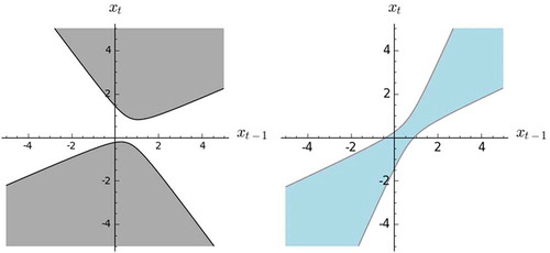If instead $\mathrm{\Delta }[{\sigma }^{-2}]$ is positive, ${\sigma }_{+}<{\sigma }_{-}$, the values of $x$ consistent with a positive log-likelihood ratio, i.e., the evidence supports $S=1$, is the union of two intervals $[-\mathrm{\infty },\underset{\_}{x}(x_{t-1})]\bigcup [\bar{x}(x_{t-1}),+\mathrm{\infty }]$.⁹ Figure 2 illustrates two possible configurations of the regions of the plane $(x_{t-1},x_t)$ where the log-likelihood ratio is positive.

Figure 2. Sign of log-likelihood ratio, Equation (13).

The two figures show how the sign of the log-likelihood ratio, given in (13), can vary across regions of the $(x_{t-1},x_t)$ plane for distinct values of the parameters. The shaded area in each case indicates the region in the plane where the log-likelihood ratio is positive, i.e. $(x_{t-1},x_t)$ increases the posterior odds in favour of $S=1$. The parameters for the regions on the left hand pane are: ${\mu }_{-}=-0.1,{\mu }_{+}=0.1,{\rho }_{-}=0.6,{\rho }_{+}=0.3,{\sigma }_{-}=0.65$ and ${\sigma }_{+}=0.55$. To produce the right hand pane, the parameters are identical except for ${\sigma }_{-}=0.55$ and ${\sigma }_{+}=0.65$.

The log-likelihood ratio at time $t$, and therefore the sum of log-likelihood ratios, does not respond to $x_t$ in a monotone fashion since:

(14) $\frac{\mathrm{\partial }ln{\lambda }_t}{\mathrm{\partial }{x}_t}=\frac{\mathrm{\partial }{\sum }_{\tau =1}^{t}ln{\lambda }_{\tau }}{\mathrm{\partial }{x}_t}=\mathrm{\Delta }\left[\frac{1}{{\sigma }^2}\right]x_t-\mathrm{\Delta }\left[\frac{\rho }{{\sigma }^2}\right]x_{t-1}-\mathrm{\Delta }\left[\frac{\mu }{{\sigma }^2}\right].$(14)

If $\mathrm{\Delta }[\frac{1}{{\sigma }^2}]>0$, that is, households believe that the price differential is more variable when the average price differential is positive, the log-likelihood ratio increases whenever $x_t>\mathrm{\Delta }[\frac{\rho }{{\sigma }^2}]/\mathrm{\Delta }[{\sigma }^{-2}]x_{t-1}+\mathrm{\Delta }[\frac{\mu }{{\sigma }^2}]/\mathrm{\Delta }[{\sigma }^{-2}]$. Hence, in this case, only a large enough $x_t$ increases the log-likelihood ratio and therefore reduces the probability to leave the variable-price contract. If instead $\mathrm{\Delta }[{\sigma }^{-2}]<0$, values of $x_t$ smaller than $\mathrm{\Delta }[\frac{\rho }{{\sigma }^2}]/\mathrm{\Delta }[{\sigma }^{-2}]x_{t-1}+\mathrm{\Delta }[\frac{\mu }{{\sigma }^2}]/\mathrm{\Delta }[{\sigma }^{-2}]$ lead to a larger log-likelihood ratio.¹⁰

Figure 3 describes two examples of the behaviour of the log-odds $ln{o}_2$, assuming that the log-likelihood ratio takes the form given in Equation (13), after three realisations of $x_t$ for two distinct parametrisations. The first two realisations are set at $x_0=0$ and $x_1=-1$ while $x_2$ is allowed to vary over the range $(-3,2)$. The figure illustrates the fact that the log-odds can be positive (or negative) and yet display either a positive or a negative slope relative to $x_2$. For $x_2=-3$, $ln{o}_2$ is positive for both parametrisations, but in one case the log-odds is an increasing function of $x_2$ at that point whereas in the other case the log-odds is a decreasing function of $x_2$. Similarly, for $x_2=1.5$, both log-odds are negative, and in one case the log-odds is increasing at that point while in the other case it is decreasing.

Figure 3. Log-odds, $ln{o}_2$ for $x_0=0$, $x_1=-1$, Equation (8).

Assuming that the first two realisations are $x_0=0$ and $x_1=-1$, the figure shows how the log-odds $ln{o}_2$, changes with $x_2$. The other parameters to define the two curves are: ${\mu }_{-}=-0.1,{\mu }_{+}=0.1,{\rho }_{-}=0.6$, and ${\rho }_{+}=0.3$.

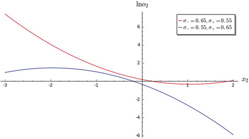
Hence, a new realisation of $x_t$ adds evidence, in the form of $ln{\lambda }_t$, to the prior log odds ${\kappa }_0+{\kappa }_{1}ln{o}_{t-1}$. It is only if $ln{\lambda }_t>0$, however, that the probability to remain on a variable-price contract increases with a new realisation of $x_t$.¹¹

2.4. Bivariate information

Assume now that the price differential and the local temperature deviations from long-term trends are observed by the decision-maker. $x_t$ is now multivariate (here bivariate). Assume that the first component, $x_{1t}$ of $x_t$, measures the local temperature deviations from long-run averages while the second component, $x_{2t}$, measures the log price differential between the variable-price and the fixed-price contracts. Because our data covers a short period of time, the households are assumed to believe that the process which describes the evolution of the local climate is independent of the state of the world which describes the evolution of the log price differential. This does not mean that the history of the local temperature at time $t$ is irrelevant, but rather that the decision-maker can use the temperature history together with price history to improve her decision concerning the state of the world. For example, extreme prices at the same time as extreme temperatures may provide a more informative signal about the state of the world than extreme prices alone.

We assume further that given the state of the world ($S$) and given the history ${\mathcal{X}}_{t-1}$ until $t-1$, we can decompose the likelihood $P[x_t|S,{\mathcal{X}}_{t-1},t]$ in terms of the product of the marginal density for the temperature information contained in $x_{1t}$, $f_1(x_{1t}|x_{1,t-1})$, and of the conditional density of the log price differential, $f_2(x_{2t}|S,x_{2,t-1},x_{1,t},x_{1,t-1})$:

(15) $Pr[x_t|S,{\mathcal{X}}_{t-1},t]=f_1(x_{1t}|x_{1,t-1})f_2(x_{2t}|S,x_{2,t-1},x_{1,t},x_{1,t-1}).$(15)

The log-likelihood ratio for the observation of $x_t$ at time $t$ then takes the simpler form:

(16) $ln{\lambda }_t=\frac{Pr[x_t|S=1,{\mathcal{X}}_{t-1},t]}{Pr[x_t|S=0,{\mathcal{X}}_{t-1},t]}=\frac{f_2(x_{2t}|S=1,x_{2,t-1},x_{1,t},x_{1,t-1})}{f_2(x_{2t}|S=0,x_{2,t-1},x_{1,t},x_{1,t-1})},$(16)

which depends only on the conditional densities given each state of the world of the log price differential. The interpretation of the history of the local temperature in Equation (15) is that temperature is informative about the prices, and therefore enters the conditional densities $f_2(x_{2t}|S=1,x_{2,t-1},x_{1,t},x_{1,t-1})$.

To extend the model specification we discussed in the univariate case, assume that the bivariate process $X_t\equiv (x_{1t},x_{2t}{)}^{\prime }$ is described by a state contingent triangular VAR(1) model of the form:

(17) $\begin{array}{cc}{x}_{1t}& ={\nu }_0+\psi x_{1,t-1}+{ϵ}_{1t},\\ x_{2t}& ={\rho }_{1S}{x}_{1,t-1}+{\rho }_{2S}{x}_{2,t-1}+{\mu }_S+{ϵ}_{2t},\end{array}$(17)

with ${\mu }_1\equiv {\mu }_{-}$, ${\mu }_0\equiv {\mu }_{+}$, ${\rho }_{k1}\equiv {\rho }_{k-}$, ${\rho }_{k0}\equiv {\rho }_{k+}$, for $k=1,2$.

We assume that the innovations ${ϵ}_t\equiv ({ϵ}_{1t},{ϵ}_{2t}{)}^{\prime }$ are conditionally normally distributed given the past information, ${\mathcal{X}}_{t-1}$. Hence, given the information about the realisation of the temperature $x_{1t}$ at time $t$, the distribution of $x_{2t}$ remains normal. However, in general, the parameters which define the conditional distribution will depend on the state of the world. Consider the form of the variance covariance matrix of the innovations given the state of the world and the past information:

(18) $\mathbb{V}[{ϵ}_t|S,{\mathcal{X}}_{t-1}]=\left[\begin{array}{cc}{\sigma }_1^2& {\omega }_S{\sigma }_1{\sigma }_{2,S}\\ {\omega }_S{\sigma }_1{\sigma }_{2,S}& {\sigma }_{2,S}^2\end{array}\right],$(18)

where ${\sigma }_{2,S}^2$ is the variance of the innovation in the definition of $x_{2t}$ given the state of the world. ${\omega }_S$ is the correlation between the innovation given the state of the world. We set ${\sigma }_{21}\equiv {\sigma }_{2-}$, ${\sigma }_{20}\equiv {\sigma }_{2+}$, ${\omega }_1\equiv {\omega }_{-}$, ${\omega }_0\equiv {\omega }_{+}$. In general, we assume ${\sigma }_{2-}\ne {\sigma }_{2+}$ and ${\omega }_{-}\ne {\omega }_{+}$. This specification guarantees that the variance of $x_{1t}$ is independent of the belief of the state of the world, while the conditional expectation and the conditional variance of ${ϵ}_{2t}$ given ${ϵ}_{1t}$ will depend on the belief of the state of the world:

(19) $\mathbb{E}[{ϵ}_{2t}|S,{\mathcal{X}}_{t-1},{ϵ}_{1t}]={\omega }_S{\sigma }_{2S}{ϵ}_{1t},$(19)

(20) $\mathbb{V}[{ϵ}_{2t}|S,{\mathcal{X}}_{t-1},{ϵ}_{1t}]={\sigma }_{2S}^2(1-{\omega }_S^2)\equiv {\tilde{\sigma }}_{2S}^2.$(20)

Given the state of the world, the history ${\mathcal{X}}_{t-1}$ and $x_{1t}$, the conditional expectation of $x_{2t}$ takes the form:

(21) $\begin{array}{rl}{x}_{2t}& ={\rho }_{1S}{x}_{1,t-1}+{\rho }_{2S}{x}_{2,t-1}+{\mu }_S\\ & +\frac{{\omega }_S{\sigma }_{2S}}{{\sigma }_1}(x_{1t}-{\nu }_0-\psi x_{1,t-1})+{\widetilde{ϵ}}_{2t}\\ & ={\tilde{\rho }}_{0S}{x}_{1t}+{\tilde{\rho }}_{1S}{x}_{1,t-1}+{\rho }_{2S}{x}_{2,t-1}+{\tilde{\mu }}_S+{\widetilde{ϵ}}_{2t},\end{array}$(21)

where ${\widetilde{ϵ}}_{2t}$ is a normally distributed innovation with conditional variance equal to $\mathbb{V}[{ϵ}_{2t}|S,{\mathcal{X}}_{t-1},{ϵ}_{1t}]$. The last expression collects the composite terms into state dependent parameters (denoted by $\sim$). The above equation shows that even in the normal case, the conditional densities $f_2(x_{2t}|S,x_{2,t-1},x_{1,t},x_{1,t-1})$, for $S=0$ and $S=1$, are described in general by parameters which depend on the state of the world (if ${\sigma }_{20}{\omega }_0={\sigma }_{21}{\omega }_1$, the conditional mean is state invariant, although the conditional variance may still be state dependent).

Adding additional information, here the information about temperature $x_{1t}$, modifies the conditional mean for the price differential $x_{2t}$ without modifying significantly the conclusions reached in Section 2.3. Further algebra gives expressions for the log-likelihood ratio that are similar to the one we discuss in Equation (13). In particular, we can show that there are regions of the space $(x_{1t-1},x_{2t-1},x_{1t},x_{2t})$ such that the log-likelihood ratio is positive, i.e., that supports the belief that the state of the world is $S=1$.

3. Data

3.1. The Swedish electricity market

Since deregulation of the Swedish electricity retail market in 1996, households are free to choose between hundreds of retailers, each offering several different contracts. Roughly $40$ per cent of all Swedish households have chosen a fixed-price contract, and another $40$ per cent have chosen a variable-price contract. Most of the remaining households are on so-called default contracts with the incumbent retailer, which households automatically are assigned to if they do not make an active choice to either a variable-price or fixed-price contract. These contracts typically have prices varying seasonally, and the price per kWh is higher than both variable-price and fixed-price contracts. The marginal price per kWh, which is constant across consumption levels, is typically between $30$ and $60$ öre (one öre is $0.1$ SEk or roughly $0.01$ Euro), with variation both across contract types and seasons. In addition to the price per kWh, households pay for transmission, green certificates and taxes, which are independent of contract choice. These costs amounts to roughly $50$ öre/kWh, plus a fixed annual transmission fee varying between $1500$ and $15000$ SEK depending on the household’s required amperage. Because prices are similar across retailers but differs between contract types, cost savings are larger from switching between contract types than from switching between retailers (Littlechild, 2006). This is apparently true for competitive markets like the Swedish retail market for electricity (e.g., Brännlund et al., 2012; Damsgaard et al., 2005), and more households switch between contracts than between retailers (see SCB, 2016).

For the Swedish retailer market, switching between contracts does not affect electricity consumption levels by any significant amount. First, the only differences between a variable-price contract and a fixed-price contract are the retail price and the price variability. The Swedish contracts do not contain contract-specific attributes such as the increasing block-rate pricing schemes typically found, for example, in the US. Second, to a large extent, electricity consumption is determined by temperature and daylight seasonality¹² together with the number and efficiency levels of the appliances used by the household; the former is obviously common to all contracts within broad regions, and the latter is typically fixed in the short run. See, for example, Vesterberg, Kiran, and Krishnamurthy (2016) for a detailed description of residential electricity demand in Sweden. Overall, electricity consumption is believed to be unaffected by the type of contract, and therefore the expenditure variation after a contract switch mostly reflects the price differential (we confirm for this for the sample at hand in the Section below).

Further, the monetary switching costs associated with switching from a variable-price contract to a fixed-price contract are zero, and households on variable-price contracts are free to switch to a fixed-price contract at any time. Households on fixed-price contracts, however, have agreed to remain on this contract for the length of the contract period, and typically they are required to pay a penalty fee to cancel their fixed-price contract ahead of time.

3.2. Skellefteå Kraft

The data used in this paper originates from the customer database of Skellefteå Kraft, one of the bigger electricity retailers in Sweden (see www.skekraft.se). The source material has been anonymised and identification of households is not possible. We use a sub-set of this data, consisting of all customers that started a variable-price contract during the period June 2010 to February 2012 and did not have an electricity contract with Skellefteå Kraft prior to this. This gives us a total sample size of $3353$ households. Although we do not observe the contract (if any) these households had prior to the sample period, we do know that the choice of variable-price contract with Skellefteå Kraft was an active choice (e.g., compared to default contracts which households are automatically assigned to if they do not make an active choice). The households in the sample have either remained on their variable-price contract throughout the sample period which ends in June 2014 (we treat these observations as right-censored), or switched to either a fixed-price contract with the current retailer, or switched to an unknown contract type with an alternative retailer, i.e., such households would have exercised their outside option (in which case we do not observe the contract type they switched to, but we know that until they left Skellefteå Kraft they were on a variable-price contract. We treat these observations as right-censored as well).

Most of the households in the sample ($76$ per cent) share the same postal area code as the retailer in northern Sweden (Skellefteå), whereas the Swedish population is concentrated in the middle and south of Sweden. The location of the households in the sample is expected, because one important determinant of retailer choice typically found to be geographical location and closeness to the retailer (see Goett et al., 2000; Revelt & Train, 2000; Yang, 2014). However, the sample contains observations on households from all $21$ postal areas in Sweden. For example, roughly 8 per cent of the households live in Stockholm, and another 3 per cent in Gothenburg.

The data includes detailed household-level information about the current electricity contracts, prices per kWh, electricity consumption in kWh, geographical location and housing type (villa or flat, and type of heating system). Unfortunately, the database lacks any household-level information about income and other household characteristics and only includes socio-economic information at the zip-code level¹³ using census data with figures (from 2014) on annual per-capita income, family size, age and education level.¹⁴ These household characteristics are used to account for household and dwelling characteristics in the initial condition $z_0$ in the model outlined above. While zip-code level census data might fail to capture heterogeneity across households, we note that most of the household characteristics typically are fixed or only vary by little in the short term (e.g., building characteristics, income and education levels), and that such characteristics are unlikely to determine the timing of the switch between contracts. Furthermore, the household characteristics that are possibly the most important determinants for electricity demand are housing type and heating system (Vesterberg et al., 2016), and we observe these characteristics at the household level. In particular, conditional on these housing characteristics, we expect households to be relatively similar in terms of both consumption levels and consumption patterns (see, for example, Figure 1 in Vesterberg et al. (2016), where it is clear that consumption levels and patterns across different end-uses are very similar across households).

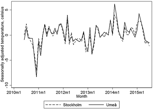
Data on temperature, which also is an important determinant for electricity consumption, is available at the postal area level (i.e., locally) from SMHI (Swedish Meteorological and Hydrological Institute; see www.smhi.se). Note that because temperature in our empirical work is measured locally, adding temperature to the information source available to the household introduces further heterogeneity between households, beyond what is captured by the zip-code level measures. Both price and temperature data are seasonally adjusted (by postal area in the case of temperature), and since price and temperature data is available from 2006, the seasonally adjusted variables may be thought of as deviations from the long-term monthly average price and temperature. Descriptive statistics of the variables used in the empirical application are found in Table 1, and the seasonally adjusted monthly temperature for Stockholm and Umeå is illustrated in Figure 4.

Table 1. Summary statistics.

	Mean	Standard deviation	Min	Max
Variable price, öre/kWh	43.35	11.21	0.21	0.927
Fixed price, öre/kWh	49.46	0.72	0.38	0.65
Temperature (Celsius)	4.58	8.18	−15.6	20.8
Monthly kWh, electrically heated villas	1473.13	1020.00	23	9515
Monthly kWh, non-electrically heated villa	964.92	869.40	2	9120
Monthly kWh, flats	735.01	843.33	1	6768
Income (1000’s SEK)	273.52	55.85	165	467
Age	49.07	4.55	35.4	66.9
Flats, share	0.79
Non-electrically heated villas, share	0.12
Electrically heated villas, share	0.09
Family size, share (more than two persons $=1$	0.34
University, share (University degree = 1)	0.22
Number of Households in sample	3353
Average Number of Months in sample	18

Note: Prices are excluding transmission, green certificate and taxes, which are independent of contract choice.

Figure 4. Seasonally adjusted temperature for Stockholm and Umeå.

The figure shows seasonally adjusted temperature (in degrees celsius, from month average) for Stockholm, located in the centre of Sweden and Umeå, located in the north of Sweden.

For the households in the sample, the variable price per kWh is lower than the corresponding fixed price, since households on the latter type of contract pays a premium to avoid monthly price variability: the average price difference is six öre/kWh.¹⁵ Furthermore, roughly $80$ per cent of the households in the sample are living in flats. For the Swedish population, the corresponding figure is less than $50$ per cent. One explanation to the large share of flats in the sample could be that variable-price contracts may be more common for flats. Electricity consumption is highest for electrically heated villas, as expected, and smaller for non-electrically heated villas and flats, and the electricity usage levels are comparable to those reported by the Swedish Energy Agency (see www.energimyndigheten.se/en). The relatively large standard deviations illustrate variation in electricity usage across seasons, with average electricity demand during winter being substantially higher than during summer. Since temperature, income, age, family size and university are zip-code level averages, these variables obviously corresponds to population figures.

Electricity consumption is more or less identical before and after any switch between a variable-price and a fixed-price contract. To show this, we compare the percentage change before and after a switch to the percentage change between any other months in our data, and find no statistically significant (at the 5 per cent level) difference in the percentage changes before and after a switch. However, we do find a significant difference in percentage change in costs (price times quantity) before and after a switch compared to the percentage change between any other months. This is precisely what we would expect if electricity consumption is unrelated to the choice of contract.

$730$ of the households in the sample have switched to a fixed-price contract with the current retailer¹⁶ (in the Swedish population, roughly $15$ per cent of the households switch between contracts each year (SCB, 2016)). As is evident from Figure 5, most of these switches occurred during 2010 and 2011, with virtually no switches during 2012. The number of switches peaked during October 2010 with about $100$ switches, corresponding to 7 per cent of the households in the data that month. Further, we observe that time-periods with many switches occur some months after positive price differentials, and that periods of negative price differentials are associated with few or zero switches, as would be expected. According to the retailer, there were no specific marketing campaigns during these periods, which otherwise could have explained the many switches. Furthermore, Statistics Sweden reports that more households switched between contracts in 2011 than during the subsequent years, so the observation in our data of more activity during 2010 and 2011 appears to be consistent with aggregate data (see SCB, 2016). The number of new variable-price contracts per month (“Entries”) varies between $70$ and $243$. Since households start their variable-price contract at different points in time, they face different histories of prices. This variation in price histories, together with the variation in temperature across location, ensures the identification of the parameters of the model. Also, note that the number of switches to the outside option (“Switches to unknown” in Figure 6) and new customers to Skellefteå Kraft (i.e., households choosing either fixed-price contracts or variable-price contracts)¹⁷ is low and less variable over time.¹⁸

Figure 5. Seasonally adjusted log price differential and number of switches per month.

”Switches to fixed-price contract” refers to switches within the same supplier to a fixed-price contract, ”Switches to unknown” refers to switches to another retailer, and ”Entries” refers to number of new variable-price contracts per month. Our sample only includes households starting a variable-price contract between June 2010 and February 2012, so number of entries in the sample are zero after February 2012. ”Price differential” is the seasonally adjusted log price differential between the variable price and the fixed price..

The proportion of households remaining on variable-price contracts over time is illustrated in Figure 6, where we illustrate the survival function for households on variable-price contracts using the Kaplan-Meier estimator. Evidently, the survival function drops rather quickly, but becomes rather flat after roughly fifteen months. Comparing with the number of switches per month in Figure 1, we observe many switches in the beginning of the sample, where the households in the sample have spent a relatively short time on the variable-price contract. Obviously, the difference between the survival function depicted in Figure 6 and the model outlined in this paper is that the latter allows us to condition the survival probability on distinct histories of information, thereby allowing us to understand the sensitivity of the probability of remaining on a variable-price contract to variation in the price and temperature histories.

4. Estimation and results

4.1. Estimation

For each household $i$ we observe a history of choices, ${\mathcal{D}}_t$, a history of the realisation of the variables measuring the information available to decision-makers up to time $T_i$, ${\mathcal{X}}_t$, as well as the variable describing the household initial conditions, $z_0$, i.e., we observe $({\mathcal{D}}_{T_i},{\mathcal{X}}_{T_i},z_0)$. The specification of the probabilities we provided earlier allow for a simple expressions to the individual contributions to the (conditional) likelihood:

(22) $\begin{array}{rl}& {\mathcal{L}}_i(({\mathcal{D}}_{T_i},{\mathcal{X}}_{T_i}),\theta )\\ & =\prod _{t=1}^{T_i}Pr[D_{it}=1|{\mathcal{X}}_t,t,z_{i0}{]}^{D_{it}}Pr[D_{it}=0|{\mathcal{X}}_t,t,z_{i0}{]}^{1-D_{it}},\end{array}$(22)

where the vector $\theta$ collects all the parameters of the model. From this expression, calculating the sample log-likelihood is straightforward.

The information vector describing the initial conditions, $z_{i0}$, includes building type (electrically heated villa, non-electrically heated villa or flat), household income level, family size (more than two persons or not), education (university degree or not) and age. The log price differential (log of variable price divided by fixed price) and temperature information is defined relative to their monthly averages (at the postal area level for temperature).

The normality assumption of the conditional distribution in either state of the world which we focus on is useful since it leads to expressions for the log-likelihood ratio which are linear in the statistics of the data. Hence, the log-odds $ln{o}_t$, which is a (weighted) sum of log-likelihood ratios, is itself a linear form of the statistics of the data $x_{1t},x_{2t}$ and their squares $x_{1t}^2,x_{1t-1}^2,x_{2t}^2,x_{2t-1}^2,$ and cross products $x_{1t}{x}_{2t},x_{1t}{x}_{1t-1},x_{2t}{x}_{2t-1},x_{1t}{x}_{2t-1},x_{1t-1}{x}_{2t}$ etc. The distributional parameters which characterise the conditional distribution in each state of the world determine the function of the parameters, i.e., the form $\mathrm{\Delta }[\frac{{\mu }^j{\rho }_l^k}{{\sigma }^2}]$, for each particular statistics that enters the log-odds. The scale of these parameters itself is in general not identified since the contribution of the log-odds to the probability to keep a variable-price contract is scaled by ${\pi }_1$. In our applied work, we do not attempt to recover the distributional parameters from the estimated parameters. Hence, the parameter $\theta$ includes both the parameters of the initial characteristics and the parameter of the trend and of the information discounting.

Table 2 summarises estimation results for a selected set of specifications. For each specification, it describes the number of parameters, the estimated trend and discount, the log-likelihood, AIC and BIC. The complete list of parameter estimates for all specifications can be found in the Appendix in Tables A1 and A2.

Table 2. Estimation summary.

Specification	(1)	(2)	(3)	(4)	(5)	(6)	(7)	(8)	(9)
No. of param.	2	2	2	3	3	3	14	14	14
Init. cond.	Yes	Yes	Yes	Yes	Yes	Yes	Yes	Yes	Yes
Trend		0.126 ***	0.152 ***		0.0708 ***	0.107 ***		−0.331 ***	−0.467 ***
		(0.007)	(0.013)		(0.008)	(0.013)		(0.040)	(0.051)
Discount			0.980 ***			0.978 ***			0.894 ***
			(0.007)			(0.005)			(0.015)
Number obs.	83786	83786	83786	83786	83786	83786	83786	83786	83786
Log-Likelihood	−3857.7	−3624.4	−3620.3	−3595.5	−3548.9	−3538.9	−3398.8	−3360.1	−3323.9
AIC	7765.3	7300.7	7294.7	7243.0	7151.8	7133.9	6867.6	6796.2	6725.8
BIC	7998.7	7543.4	7546.8	7485.7	7403.9	7395.3	7213.0	7151.0	7089.9

i) The table report maximum likelihood estimates based on the maximisation of expression (22) on the information in the sample. All specification accounts for the same initial characteristics. The number of parameters in the model of the log-likelihood ratio is reported in the second row.

ii) Columns 1–3 report on the estimation results for the univariate homoskedastic model of the log-likelihood ratio (described in Equation (A3)) where the information is the log price differential only. Column 4–6 report results for the univariate homoskedastic model (described in Equation (A3) in the Appendix A.2) where the mean log-price differential at time t depends on the local temperature deviation from monthly means. Column 7–9 report results for the bivariate heteroskedastic model where the information is both the log price differential and the temperature deviations from monthly averages. We report separately the estimates of the trend and discount parameters and their standard errors (in parentheses).

iii) The number of observations refer to the number of individuals $\times$ months observed in the sample.

iv) The log-likelihood statistics, Akaike’s and Schwarz’s Bayesian information criteria statistics are reported for each model. While a larger log-likelihood suggests a better fit, a smaller value of either information criteria suggests a better model. The information criteria penalise the fit with the number of parameter used.

Consider first the simple model (column 1): the homoscedastic model without any trend or discounting, and where the auto-correlation coefficients are the same for both state contingent data generating process. The results for this specification implies that households respond to a weighted sum of prices, and in particular that household will interpret a large price differential as evidence against the variable-price contract. We find that introducing a trend term (column 2) as well as information about the local weather (column 4 and 5) improves the fit (as measured by the likelihood), relative to the simpler alternative specification. Allowing for some discounting (column 3 and 6) in the dynamic of the log-odds increases the likelihood further, although the discounting parameter remains close to one in value. Allowing the data generating process for the price differential to include state contingent auto-correlations and variances (as described in Equation (21)) improves the fit further. The information criteria measures (AIC or BIC) suggest that the additional parameters in this specification improve the quality of the model fit further. In summary, the evidence supports the hypothesis that households process the information contained in price histories in a complex fashion.

Finally, the evidence obtained from fitting the homoscedastic model specification appears to reject the null hypothesis that households respond to the current price differential when they choose whether or not to switch to the fixed-price option. This hypothesis requires that the parameter for the lagged price differential and the discount parameter is equal to zero. However, the parameter estimates we provide in the appendix in Tables A1 and A2 show that the discount parameter is precisely estimated away from zero, and than past values of the price differential contain useful information and improve the fit of the model¹⁹.

For each specification, Table 2 reports the estimated values for the trend and the discount parameters. These parameters are precisely estimated in all cases. While the discount rate is estimated to be close to unity in all cases, the parameter estimates for the trend vary between specifications and is negative with the most complex specification. In a first approximation, we interpret the parameter of the trend as the parameter ${\kappa }_0$ in Equation (9).²⁰ When ${\kappa }_0$ is negative, the decision-maker scales down the posterior odds she reached at the end of period $t$ towards zero to produce her prior odds at the start of period $t+1$. The parameter estimate in the last column; ${\kappa }_0=-0.467$, amounts to scaling down the posterior odds by $0.63$. Together with the estimated discount rate, the results for the last specification suggest that decision-makers forget past evidence and systematically downplay the information in favour of variable prices by a considerable factor.

The estimated parameters of the log-likelihood ratio are not straightforward to interpret. This is true in particular for the heteroscedastic models where there are many higher order and interaction terms. We argue that a more constructive way to understand the results is to produce survival functions for distinct price levels which illustrate the behaviour of the model to distinct histories of prices.

4.2. Duration analysis

The probabilities for a household to switch from a variable-price contract to a fixed-price contract exactly at time $\tau$, or after time $\tau$, given a history of information ${\mathcal{X}}_{\tau }$, are

(23) $Pr[Exit=\tau |{\mathcal{X}}_{\tau },z_0]=\prod _{k=1}^{\tau -1}{P}_k^1\cdot P_{\tau }^0,$(23)

(24) $Pr[Exit>\tau |{\mathcal{X}}_{\tau },z_0]=\prod _{k=1}^{\tau }{P}_k^1,$(24)

with $P_t^1\equiv Pr[D_t=1|{\mathcal{X}}_t,t,z_0]$ and $P_t^0\equiv 1-P_t^1$.

The last two expressions show the relationship between the conditional exit probabilities we discussed in Equation (4) and the probability that an exit from the variable-price contract takes place after or exactly at some time $\tau$. Current, future and past probabilities to leave a variable-price contract are related, and we must have:

(25) $Pr[Exit>\tau |{\mathcal{X}}_{\tau },z_0]+Pr[Exit=\tau |{\mathcal{X}}_{\tau },z_0]=Pr[Exit>\tau -1|{\mathcal{X}}_{\tau -1},z_0],$(25)

since

$Pr[D_{\tau }=1|{\mathcal{X}}_{\tau },\tau ,z_0]+Pr[D_{\tau }=0|{\mathcal{X}}_{\tau },\tau ,z_0]=1,$

That is, at any time $t$ either the household remain on the variable-price contract or exits it (to a fixed-price one).²¹

The discrete survival function given in Equation (24) describes the survival probability up to time $t$ given a specific history ${\mathcal{X}}_t$ of the information. Denote $\mathcal{P}(\mathcal{X})$ the sequence of survival probabilities given a complete history of information $\mathcal{X}$ from $t=1$ to $t=+\mathrm{\infty }$, that is:

$\begin{array}{rl}P(\mathcal{X})& =(Pr[Exit>1|\mathcal{X},z_0],Pr[Exit>2|\mathcal{X},z_0],\dots ,\\ & Pr[Exit>+\mathrm{\infty }|\mathcal{X},z_0])\\ & =(Pr[Exit>1|{\mathcal{X}}_1,z_0],Pr[Exit>2|{\mathcal{X}}_2,z_0],\dots ,\\ & Pr[Exit>t|{\mathcal{X}}_t,z_0]),\dots ,\\ & Pr[Exit>+\mathrm{\infty }|\mathcal{X},z_0]),\end{array}$

where the second expression stresses that the $t^{th}$ probability of $\mathcal{P}(\mathcal{X})$ depends on the history up to time $t$ only. Clearly each element of $\mathcal{P}(\mathcal{X})$ is a probability, and furthermore, Equation (25) implies that the sequence is (weakly) decreasing. Hence, we can consider the expected sequence of survival probabilities, $\mathcal{P}$, over all possible histories of the information:

$\mathcal{P}\equiv \underset{\mathcal{X}}{\mathbb{E}}[\mathcal{P}(\mathcal{X})].$

Direct examination of the elements of $\mathcal{P}(\mathcal{X})$ suggests that the $t^{th}$ element of $\mathcal{P}$ can be expressed as:

(26) ${\mathcal{P}}_t=\underset{\mathcal{X}}{\mathbb{E}}[Pr[Exit>t|{\mathcal{X}}_t,z_0]]=\underset{{\mathcal{X}}_t}{\mathbb{E}}[Pr[Exit>t|{\mathcal{X}}_t,z_0]].$(26)

We can therefore use the parameter estimates to construct an estimate of $\mathcal{P}$ provided that we describe the data generating process which creates the histories $\mathcal{X}$.

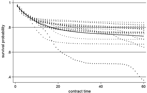
Figure 7 illustrates such a construction for the homoscedastic model which accounts only for the history of price differentials, and where the log-odds are determined according to the modified Bayesian updating procedure we describe in Equation (9). To obtain the figure, we estimate a simple time series model on the observed history of the (deseasonalised log of the) variable prices (see Table A3 in the Appendix for more details). In this case, the simplest model takes the form of an AR(1) model. We then calculate the standardised residuals. We set the fixed price to $50$ öre/kWh, and we draw from the residuals independently and with replacement an alternative history of the variable price innovations, which we use together with the estimated model to generate an alternative history of the variable price from July 2009 until June 2014. Hence, the variable price and fixed price together allow us to generate an alternative history of the price differential. Figure 7 shows the effect of several (fifteen) such possible alternative histories on the survival probabilities (the dotted lines), as well as the average over all possible histories of the survival probabilities (the continuous line).

Figure 6. Kaplan-Meier survival estimate.

The figure shows the Kaplan-Meier estimator for the proportion of households remaining on variable-price contracts over time.

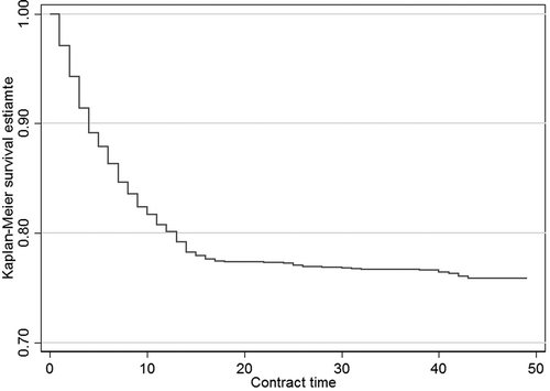
A first thing to notice is that the shape of the survival functions in Figure 7 all resembles the shape of the Kaplan-Meier survival function in Figure 6. In particular, there is a sharp decrease in the survival probability for short durations, and the survival function thereafter becomes almost flat. However, it is noticeable that distinct histories of the price differential yield a considerable range of the proportion that survive with a variable-price contract after sixty months, since it ranges from below $40$ per cent to more than $80$ per cent. It is the timing of large positive shocks to the price differential during a particular history which determines variation to the proportion remain on a variable-price contract: if the large shocks arise early, the proportion of survivors is smaller than if the large shocks arise later in the history.

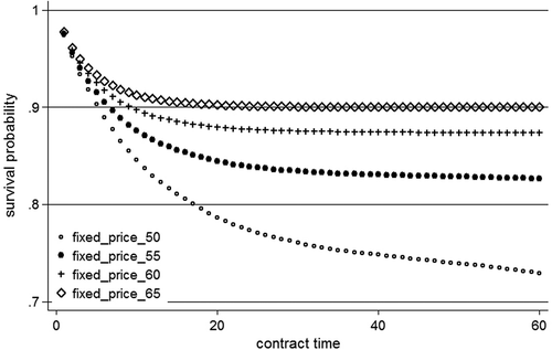
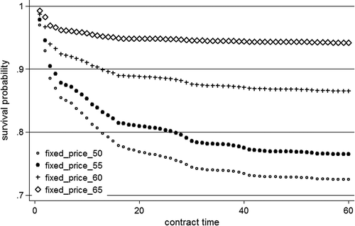
We now focus on the implication of the model using the specification with the best fit; that is, the specification which accounts for the history of the price differential and the history of temperature with the model of modified Bayesian updating as given in column (9) in Table 2. We repeat the simulation procedure for different fixed prices (i.e., draw $250$ histories for the variable price process, and generate the price differential given the fixed price, and then average over the conditional survival probabilities). We then generate the average survival sequence when the history of the information relevant to the household contains the price differential and the temperature deviations from the household local monthly average.

We estimate a time series model of the (log of the) variable price, which conditions on last month variable price as well as on the current and the previous month deviation from the local temperature average (for the calculation presented this model is estimated assuming the household is located in Umeå). From the standardised residuals of this model, keeping the history of the local weather to its observed values, we generate alternative histories of the variable price.

Over the period 2003 to 2014 (June), the fixed-price offers range between $38$ and $69$ öre/kWh. However, we observe in Figure 1 that at the start of our sample period (June 2010) the fixed-price rise from about $50$ to $65$ öre/kWh (February 2011) and decreases continuously thereafter to reach $40$ öre/kWh by the end of our sample. The latest entry in our sample takes place in January 2012 when the fixed price was back at $50$ öre/kWh. Hence, we let the fixed price vary between $50$ and $65$ in increments of $5$ öre since the observed entries to variable-price contracts arise only over that price range.

Figure 7. Average survival vs. history specific survival function.

The figure shows the average (over 250 possible histories of the variable price, continuous line) survival function (survival with a variable-price contract) at price $50$ öre/kWh against the survival function for 15 distinct variable price histories (dotted lines) based on the model specification which includes price information only and allows for information discounting.

Figure 8shows the result of these calculations for an average household, i.e., a household at the sample mean for $z_0{\hat{\pi }}_0$ experiencing the temperature history of Umeå. As in the earlier simulation experiment, the sequences of survival probabilities are broadly convex functions of the contract time. The regular non-convexities to the survival probabilities, that we observe in all cases, reflect the (yearly) seasonal shocks to temperature. Furthermore, the survival functions for the distinct fixed prices are ordered and, as expected, show more response when the fixed price is small ($50$ öre/kWh) than when it is close to the maximum observed in the sample ($65$ öre/kWh). Five years after contracting, less than $75$ per cent of households still remain on a variable-price contract if the fixed price is set at $50$ öre/kWh, while more than $90$ per cent of households still remain on a variable-price contract if the fixed price is set at $65$ öre/kWh. The more elaborate model specification used here therefore suggests that the switching process responds systematically to different price histories.²²

Figure 8. Average survival function, price and temperature information, heteroscedastic information.

The figure shows the average (over 250 possible histories of the variable price) survival function (survival with a variable-price contract) for different fixed prices based on the model specification which includes price and temperature information and allows for information discounting.

5. Conclusion

The focus of this paper is to understand how households decide between remaining on their current electricity contract or switching to an alternative contract. In particular, we explore how sensitive the timing of switches away from the variable-price contract is to current and past prices. As far as we are aware, this paper is the first to explore this question for the choice between electricity contracts. To that effect, we propose a model for time series of binary decisions which allow for the dependence on the history of prices, or more generally, a history of information. Compared to a less elaborate model which would rely only on current prices, our model illustrates how a potentially long sequence of past information (in our case, prices and temperature), summarised into a parameterised log-likelihood ratio, can determine the decision. This capture in a simple fashion the intuition that a decision-maker needs to be convinced by observable facts before she agrees to change her mind about her current contract. We show furthermore that maximum likelihood estimation of the parameters of the decision model is feasible.

We provide several novel insights: First, we observe that it is the specification of the subjective price processes that determines the kind of evidence which favours the state of the world when the variable-price contract is preferable to the fixed-price contract (in the sense that it increases the posterior odds that $S=1$). Therefore, it is not necessarily the case that households interpret higher variable prices as evidence that a fixed-price contract is preferable. Intuitively, if the decision-maker believes the autocorrelation to be negative, a high relative price today would suggest a low relative price next month.

Second, we find that households do respond to new information, but that households do not respond immediately to this new information, and that it is the accumulated information that determines the switching rate. A simpler model which only estimated the effects of current prices would therefore underestimate the price responsiveness. Our results thus reinstate price as an important determinant for contract switching, and in particular shows that consumers respond to them, although not in the conventional way. Further, we illustrate how the seemingly small response to the price differential in the population may be a result of the characteristics of the information available to the households; e.g., the relatively small variability in the price differential. In particular, we illustrate how alternative price histories generate distinct patterns of transitions over time. For example, in the homoskedastic specification, roughly 75 per cent of households would still remain on a variable-price contract after sixty months if the fixed price is set at $50$ öre/kWh, while 90 per cent would still remain on a variable-price contract if the fixed price is set at $65$ öre/kWh. The heteroskedastic specification (when the autocorrelation coefficients and the variance of the innovation depends on the state of the world) produces an even larger range of the proportion of households that remain on a variable-price contract after sixty months. The results also illustrate that most of the response to prices occur within the first two years, and that decision-makers downplay old information.

From the retailers’ perspective, the results have important implications. If households were completely price inelastic in terms of switching behaviour, the firm could use this to extract consumer surplus. However, because households respond to prices, as illustrated in this paper, the retailers’ needs to take this into account when setting contract prices. For example, the value of a contract to the retailer will depend on the duration spent on the contracts, conditional on prices, and the retailer will face a trade-off between the share of households on each contract and the value of contracts. While decreasing the fixed price makes more households switch to the fixed-price contract, decreasing the fixed price also means that the value to the retailer of a fixed-price contract relative to the variable-price contract decreases. However, if the retailer want households to switch to a fixed-price contract, our results suggest that short-term pricing and discount campaigns for fixed-price contracts (e.g., reducing the fixed price during a month) may have little immediate effect on switching behaviour, especially if the price differential in the surrounding months is in favour of the households current variable-price contract, or if the temporary price decrease is relatively small. Rather, if the firm wants households to switch to a fixed-price contract, it either needs to keep the fixed price low for many consecutive months, or reduce it by a substantial amount. The firm therefore faces a trade-off between the size of the reduction of the fixed price against the length over which it is prepared to maintain a lower price offer. Note, however, that while a large temporary decrease of the fixed price reduces the firms revenues from those households who do switch, a long term but smaller reduction in the fixed price reduces the revenues to a lesser extent, which is good news for the firm. The observation that it takes time for households to be convinced to switch may also make switching behaviour less predictable for the firm. These are direct implications of the findings of our paper, and would not be obvious with a simpler model that only accounts for contemporaneous prices.

From a policy perspective, the finding that households do respond to prices by switching between contracts, albeit the response is delayed in time, suggest that switching between contracts is an important margin of price responsiveness which should be accounted for when evaluating demand response for residential electricity demand. Although the switching rate appears to be small in the population, it may be substantial for alternative price processes, as already noted. In particular, the ongoing change in the production mix of electricity generation in the Nordic market, with an increasing share of intermittent generation, will most likely result in alternative price processes with more volatile prices, and possibly also changes in the price levels. The response to such alternative price processes may have substantial effects on the composition of share of households on each type of contract.

Correction Statement

This article has been republished with minor changes. These changes do not impact the academic content of the article.

Acknowledgments

The authors would like to thank David Sundström, David Granlund, Bertrand Koebel and seminar participants at the World Congress of Environmental and Resource Economics, the Energy Transition workshop in Oslo, Managi Lab at Kyushu University and The Economic Policy Network at Umeå University for helpful comments and suggestions. Mattias is grateful for funding from the Swedish Energy Agency, grant number 44340-1. During his PhD, Mattias was funded through the Industrial Doctoral School, Umeå University, in collaboration with Skellefteå Kraft.

Disclosure statement

No potential conflict of interest was reported by the authors.

Additional information

Funding

This work was supported by the The Swedish Energy Agency [44340-1].

Notes

1. Furthermore, the data used in this paper also includes substantially more switches from variable-price contracts to fixed-price contracts than the other way around. Public data on contract switching (e.g., SCB, 2016) provides no information about the direction of switches in the population.

2. Because the retail market is competitive and prices are similar across retailers (see Section 3.1), we do not include the price of competing retailers’ contracts.

3. In other words, given ${\mathcal{X}}_{t-1}$, the observed history of the realisations of the exogenous process $X_t$ since $t=0$ up to time $t-1$, observing $x_t$ is not sufficient to decide whether $S=0$ or $S=1$ with probability 1.

4. In the Appendix, we also explain how the decision problem can be restated to fit the formalism of a conventional Markov decision process when the state of the world is not known.

5. Equation (3), or equivalently, the specification detailed in Equation (5), is providing a further restriction on the specification of the expected costs which simplifies our empirical work.

6. When ${\kappa }_0=0$ and ${\kappa }_1\to 1$ this expression agrees with Equation (8).

7. Hence, the model we develop here is not assuming that households necessarily consider or believe in the “true” model that generates the data. A more advanced theory would integrate a search through possible models.

8. When ${\sigma }_{-}<{\sigma }_{+}$, the quantity $ln(\frac{{\sigma }_{+}}{{\sigma }_{-}})+\frac{1}{2}\mathrm{\Delta }[\frac{{\mu }^2}{{\sigma }^2}]$ is always positive.

9. The intersection between the two intervals is empty if $ln(\frac{{\sigma }_{+}}{{\sigma }_{-}})+\frac{1}{2}\mathrm{\Delta }[\frac{{\mu }^2}{{\sigma }^2}]$ is negative.

10. Clearly, if ${\sigma }_{-}={\sigma }_{+}$, then $\mathrm{\Delta }[{\sigma }^{-2}]=0$. The analysis simplifies in that case, see Appendix A.2 for the analysis of the homoscedastic case.

11. Although it may be obvious to the reader, we stress that realisations of $x_t$ such that $ln{\lambda }_t>0$ can arise whether $\frac{\mathrm{\partial }ln{\lambda }_t}{\mathrm{\partial }{x}_t}>0$ or $\frac{\mathrm{\partial }ln{\lambda }_t}{\mathrm{\partial }{x}_t}<0$ so that the marginal effect of $x_t$ on the probability can be negative or positive although the evidence increased the probability to stay. The marginal effect does not measure the effect of $x_t$ on the probability to stay, i.e., whether the evidence increases or decreases the probability, but it measures how much larger or smaller the probability would be if the evidence was infinitesimally larger.

12. Sweden’s territory is located in the upper half of the northern hemisphere, between N${55}^{\circ }$ and N${70}^{\circ }$ latitude north. By comparison, New York’s latitude is N${40.7}^{\circ }$, Anchorage is N${61.2}^{\circ }$, while Stockholm and Umeå are, respectively, N${59.3}^{\circ }$ and N${63.8}^{\circ }$. Temperatures and daylight hours are therefore very variable over the year and between the north and the south of Sweden.

13. For the whole of Sweden, the average number of persons in each zip-code is $918$, allowing for precise neighbourhood matching with census data. Matching individual-level data with zip code-level data is frequently used in economics, including residential electricity demand (Borenstein, 2012; Ito, 2014).

14. Specifically, income and age are coded as dummy variables for income and age groups ($10$ groups each based in income and age distributions), family size is a dummy variable taking the value one if more than $30$ per cent of the households in a zip-code area have two or more inhabitants, and education is defined as a one if more than $40$ per cent of the people in the zip-code area has a university degree.

15. Multiplying the average price differential with the average monthly electricity consumption shows that the average cost differential between the two contracts is, on average, $88$ SEK per month for an electrically heated villa.

16. $D=0$ only when a switch from a variable-price contract to a fixed-price contract (with Skellefteå Kraft) is observed.

17. For simplicity, only entries to variable-price contracts is illustrated in Figure 5.

18. According to SCB (2016), this is also the case for the Swedish population.

19. The evidence shown in column (3) in Table A1 for example, shows that past values of the parameter for the lagged price differential is significantly different from zero, and furthermore, that the discount parameter is precisely estimated at 0.98. Hence, there does not seem to be any evidence that supports the null hypothesis that these parameters are both equal to zero.

20. Note that in general the log-likelihood ratio contains a constant term which will accumulate in the log-odds and yield a time-dependent function which is identical the last term of Equation (9). It is not possible to identify separately this constant term from ${\kappa }_0$.

21. In a more complete analysis, we would account for all causes of exit, i.e., the firm could loose the contract altogether to a competitor.

22. A similar simulation experiment performed using the simpler homoscedastic specification, which does not rely on the temperature information, generates survival curves with qualitatively comparable relative positions and profiles, see Figure 9.

23. Hence, the model we develop here is not assuming that households necessarily consider or believe in the “true” model that generates the data. A more advanced theory would integrate a search through possible models.

Appendix A

A.1. Markov decision process interpretation

We can restate the decision problem to fit the formalism of a conventional Markov decision process when the state of the world is not known.

Assume that the effect of the price does not affect the quantity of electricity consumed and set that quantity to $q(z_0)$. To simplify, assume further that the choice of switching from a variable-price contract to a fixed-price one is permanent. Variable prices at time $t$ are denoted ${\mathrm{P}}_{1t}$ and the fixed price is ${\mathrm{P}}_0$ which, to simplify, we assume fixed for all times. Given some prior probabilities about the correct state of the world at the start of period $t$, the objective of the household is to determine a policy ${\mathcal{D}}_t\equiv (d_t,d_{t+1},d_{t+2},...,d_T)$, with $d_t\in \{0,1\}$, at time $t$ for present and future decisions which minimises the expected discounted costs given the evidence, ${\mathcal{X}}_t$, observed so far:

(A1) $\text{matrix{ {C({{mathcal X}\_t},t)} \& { = mathop {min }limits\_{{{mathcal D}\_t}} ,,q({z\_0}){{mathop {mathbb E}limits\_t[sumlimits\_{tau = 0}^T ,{beta ^tau }({{rm{P}}\_{1t + tau }}prodlimits\_{k = 0}^tau {d\_{t + k}} break quad quad quad quad quad quad quad quad + {{rm{P}}\_0}(1 - prodlimits\_{k = 0}^tau {d\_{t + k}}))|{{mathcal X}\_t},{z\_0},t].} cr }}$(A1)

The expectation sign captures the uncertainty about future realisations of the variable price, as well as the uncertainty about the state of the world. Implicitly, the decision-maker is assumed to update her belief about the state of the world as new information arises. We can rewrite this expression in terms of the decision at time $t$ and the expected cost at time $t+1$:

$\begin{array}{cc}\hspace{0.17em}& C({\mathcal{X}}_t,t)=\underset{d_t}{min}q(z_0)\{\underset{t}{\mathbb{E}}[d_t({\mathrm{P}}_{1t}+\beta C({\mathcal{X}}_{t+1},t+1))+(1-d_t)\sum _{\tau =0}^T{\beta }^{\tau }{\mathrm{P}}_0|{\mathcal{X}}_t,z_0,t]\}=\\ \hspace{0.17em}& \underset{d_t}{min}q(z_0)\{Pr[S=1|{\mathcal{X}}_t,z_0,t](d_t\underset{t}{\mathbb{E}}[{\mathrm{P}}_{1t}+\beta C({\mathcal{X}}_{t+1},t+1)|S=1,{\mathcal{X}}_t,z_0,t]+(1-d_t)\sum _{\tau =0}^T{\beta }^{\tau }{\mathrm{P}}_0)\\ \hspace{0.17em}& +Pr[S=0|{\mathcal{X}}_t,z_0,t](d_t\underset{t}{\mathbb{E}}[{\mathrm{P}}_{1t}+\beta C({\mathcal{X}}_{t+1},t+1)|S=0,{\mathcal{X}}_t,z_0,t]+(1-d_t)\sum _{\tau =0}^T{\beta }^{\tau }{\mathrm{P}}_0)\}.\end{array}$

We can then identify the expected conditional costs so that $C(D=1|S=k,{\mathcal{X}}_t,z_0,t)=q(z_0){\mathbb{E}}_t[{\mathrm{P}}_{1t}+\beta C({\mathcal{X}}_{t+1},t+1)|S=k,{\mathcal{X}}_t,z_0,t]$ for $k=0,1$, where ${\mathbb{E}}_t[]$ indicates that the expectation at time $t$ is conditional on the state of the world $k$, the history ${\mathcal{X}}_t$ as well as the initial conditions $z_0$. Finally, observe that the costs of remaining with a variable-price contract $C(D=1|S=k,{\mathcal{X}}_t,z_0,t)$ effectively accounts for the option of switching to the fixed-price contract in the future.

The decision rule at time $t$ that this model generates will take a form similar to the decision rule we described in the previous section. The decision rules will be identical if we assume furthermore that $C(D=1|S=k,{\mathcal{X}}_t,z_0,t)\equiv C(D=1|S=k,z_0,t)$, i.e., the expected costs of a variable price contract is not revised with new information.

A.2. Univariate Homoscedastic Information

To simplify the analysis in the text to the homoscedastic case, assume that given $x_{t-1}$, households believe that, conditional on the past and the state of the world, $x_t$ is generated by an autoregressive model with normal innovations so that²³:

(A2) $\begin{array}{rl}& x_t\sim \mathcal{N}({\rho }_{-}{x}_{t-1}+{\mu }_{-},{\sigma }^2)\mathrm{i}\mathrm{f}S=1,\\ & x_t\sim \mathcal{N}({\rho }_{+}{x}_{t-1}+{\mu }_{+},{\sigma }^2)\mathrm{i}\mathrm{f}S=0,\end{array}$(A2)

such that the mean of the process as well as the parameter of autoregression depends on the state of the world. In our context, while it may be sensible to assume that if the state of the world is $S=0$, ${\mu }_{+}$ is positive, and if $S=1$ then ${\mu }_{-}$ is negative, this is not required.

Because of the normality assumption, the likelihood ratio for the observation of $x_t$ given the history of realisations of the process, ${\mathcal{X}}_{t-1}$, takes the form:

(A3) $\begin{array}{rl}ln{\lambda }_t& \equiv ln\frac{P[x_t|S=1,{\mathcal{X}}_{t-1},t]}{P[x_t|S=0,{\mathcal{X}}_{t-1},t]}\\ & =-\frac{1}{2{\sigma }^2}((x_t-{\rho }_{-}{x}_{t-1}-{\mu }_{-}{)}^2-(x_t-{\rho }_{+}{x}_{t-1}-{\mu }_{+}{)}^2)\\ & =-\frac{1}{{\sigma }^2}(\mathrm{\Delta }\rho x_{t-1}+\mathrm{\Delta }\mu )(x_t-\bar{\rho }{x}_{t-1}-\bar{\mu }),\end{array}$(A3)

where $\mathrm{\Delta }\mu \equiv {\mu }_{+}-{\mu }_{-}$, $\mathrm{\Delta }\rho \equiv {\rho }_{+}-{\rho }_{-}$ and $\bar{\mu }\equiv \frac{1}{2}({\mu }_{+}+{\mu }_{-})$.

The recent evidence, $x_t$, favours $S_t=1$ (in the sense that it increases the posterior odds that $S_t=1$) if i) $x_t$ is small enough when $\mathrm{\Delta }\rho x_{t-1}+\mathrm{\Delta }\mu >0$, i.e., $x_t\le \rho x_{t-1}+\bar{\mu }$, since in that case $ln{\lambda }_t\ge 0$; or ii) if $x_t$ is larger than $\rho x_{t-1}+\bar{\mu }$, whenever $\mathrm{\Delta }\rho x_{t-1}+\mathrm{\Delta }\mu <0$. Although the log-likelihood ratio response to the current realisation of the information depends on the past realisations, the weight of evidence in favour of remaining with the variable-price contract increases as long as $ln{\lambda }_t$ is positive. Figure A1 illustrates how the sign of the likelihood ratio vary across the $(x_{t-1},x_t)$ plane for two distinct configurations of the parameters. Observe that the regions of the plane $(x_{t-1},x_t)$ such that the log-likelihood ratio is positive, i.e., the current observation supports the state of the world where the variable price is cheaper, can vary markedly depending on the parameter values.

Figure A1. Sign of log-likelihood ratio, Equation (A3).

The two figures show how the sign of the log-likelihood ratio, given in Equation (A3), varies across regions of the $(x_{t-1},x_t)$ plane. The dotted and the dashed lines are the limits of the regions. In both figures, on the left (resp. right) of the dotted line the elasticity ${\eta }_{\lambda |x_t}$ is negative for all values of $x_t$ if $\mathrm{\Delta }\rho >0$ (resp. $\mathrm{\Delta }\rho <0$).

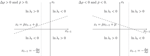
The expression of the elasticity of the likelihood ratio w.r.t $x_t$ provides an alternative understanding of the effect of the current information on the probability to remain on a variable-price contract:

(A4) ${\eta }_{\lambda |x_t}=-\frac{1}{{\sigma }^2}(\mathrm{\Delta }\rho x_{t-1}+\mathrm{\Delta }\mu ),$(A4)

Hence, the elasticity of the likelihood ratio w.r.t. $x_t$ is positive if $\mathrm{\Delta }\rho x_{t-1}+\mathrm{\Delta }\mu$ is negative, and it is positive otherwise. The response of the likelihood ratio is independent of the current information: it increases whenever $\mathrm{\Delta }\rho x_{t-1}<-\mathrm{\Delta }\mu$ and decreases otherwise. Moreover, it is possible to find a couple of observations $(x_{t-1},x_t)$ for which the elasticity ${\eta }_{\lambda |x_t}$ is negative and the log-likelihood ratio is positive.

Finally, in the special case where $\mathrm{\Delta }\rho =0$ and $\mathrm{\Delta }\mu >0$, where the autoregressive parameter is identical in the two states of the world and the price differential is negative when the variable price is preferable and positive otherwise, the log-likelihood ratio decreases with larger values of $x_t$. That is, the larger the value of $x_t$, the larger the evidence against the state where the variable price is preferable to the fixed price on average.

A.3. Parameter estimates

Table A1. Parameter estimates for specifications with univariate homoskedastic information (spec 1, 2 and 3) and bivariate homoskedastic information (spec 3, 4 and 5). 1.

	(1)	(2)	(3)	(4)	(5)	(6)
$x_{2,t}$	0.123	1.045 ***	1.297 ***	−1.406 ***	−0.407	−0.178
	(0.169)	(0.177)	(0.208)	(0.188)	(0.215)	(0.239)
$x_{2,t-1}$	−0.960 ***	−1.566 ***	−1.864 ***	−0.670 ***	−1.133 ***	−1.546 ***
	(0.169)	(0.176)	(0.213)	(0.171)	(0.181)	(0.216)
$x_{1,t}$				−0.153 ***	−0.106 ***	−0.118 ***
				(0.008)	(0.009)	(0.010)
Constant	4.719 ***	3.622 ***	3.690 ***	4.367 ***	3.854 ***	3.819 ***
	(0.371)	(0.373)	(0.373)	(0.374)	(0.376)	(0.376)
Trend		0.126 ***	0.152 ***		0.0708 ***	0.107 ***
		(0.007)	(0.013)		(0.008)	(0.013)
Discount			0.980 **			0.978 ***
			(0.007)			(0.005)
Number obs.	83786	83786	83786	83786	83786	83786
Log-likelihood	−3857.7	−3624.4	−3620.3	−3595.5	−3548.9	−3538.9
AIC	7765.3	7300.7	7294.7	7243.0	7151.8	7133.9
BIC	7998.7	7543.4	7546.8	7485.7	7403.9	7395.3

Standard errors in parentheses

* $p<0.05$, ** $p<0.01$, *** $p<0.001$

The table presents the parameters estimates for the transition model described in the main section of the paper assuming that the information is homoskedastic. $x_{1t}$ refers to the local temperature information (measured in deviations from local seasonal averages), and $x_{2t}$ refers to the price differential information (measured in deviations from seasonal averages). Specifications 1,2 and 3 present estimates assuming that the only relevant information is contained in the relative price differential. Specifications 4,5 and 6 add temperature to the relevant information.

Table A2. Parameter estimates for specifications with heteroskedasticity.

	(7)	(8)	(9)
$x_{2,t}^2$	0.609	10.55 ***	19.29 ***
	(1.705)	(2.404)	(3.632)
$x_{2,t}{x}_{1,t}$	−0.234	0.334	1.057 **
	(0.190)	(0.218)	(0.343)
$x_{2,t}{x}_{1,t-1}$	−0.580 **	−0.676 ***	0.010
	(0.192)	(0.197)	(0.258)
$x_{2,t}{x}_{2,t-1}$	−12.76 ***	−18.13 ***	−21.02 ***
	(2.673)	(2.910)	(3.507)
$x_{2,t}$	0.684 *	0.351	1.512 ***
	(0.304)	(0.321)	(0.414)
$x_{2,t-1}^2$	4.010 **	9.945 ***	14.90 ***
	(1.542)	(1.827)	(2.332)
$x_{2,t-1}$	−2.331 ***	−0.327	−0.944 *
	(0.296)	(0.386)	(0.455)
$x_{1,t}^2$	0.016 *	0.029 ***	0.065 ***
	(0.007)	(0.007)	(0.012)
$x_{1,t}{x}_{1,t-1}$	−0.053 ***	−0.065 ***	−0.049 **
	(0.011)	(0.01)	(0.015)
$x_{1,t}{x}_{2,t-1}$	0.488 ***	0.329 **	1.059 ***
	(0.122)	(0.125)	(0.189)
$x_{1,t}$	−0.076 ***	−0.055 *	−0.094 ***
	(0.021)	(0.022)	(0.027)
$x_{1,t-1}^2$	−0.014	0.002	0.0379 **
	(0.008)	(0.008)	(0.012)
$x_{1,t-1}{x}_{2,t-1}$	−0.809 ***	−0.294	−0.093
	(0.171)	(0.197)	(0.265)
$x_{1,t-1}$	0.021	0.092 ***	0.174 ***
	(0.022)	(0.024)	(0.032)
Constant	3.755 ***	3.899 ***	3.296 ***
	(0.378)	(0.378)	(0.382)
Trend		−0.331 ***	−0.467 ***
		(0.040)	(0.051)
Discount			0.894 ***
			(0.015)
Number obs.	83786	83786	83786
Log-likelihood	−3396.8	−3360.1	−3323.9
AIC	6867.6	6796.2	6725.8
BIC	7213.0	7151.0	7089.9

Standard errors in parentheses

*$p<0.05$, ** $p<0.01$, *** $p<0.001$

The table presents the parameters estimates for the transition model described in the main section of the paper assuming that the information is heteroskedastic. $x_{1t}$ refers to the local temperature information (measured in deviations from local seasonal averages), and $x_{2t}$ refers to the price differential information (measured in deviations from seasonal averages).

Table A3. Autoregressive models, ($ln$) variable price.

	Price only	Price and temperature
Constant	0.060	0.044
	(0.095)	(0.079)
$ln$ Variable price ($t-1$)	0.786 ***	0.769 ***
	(0.089)	(0.096)
Temperature ($t$)	–	−0.030 ***
		(0.007)
Temperature ($t-1$)	–	−0.018 ***
		(0.007)
$\sigma$	0.156 ***	0.136 ***
	(0.013)	(0.011)
Log-likelihood	26.37	34.79
Q-test stat	4.36	4.95
p-value (10 d-o-f)	0.93	0.90

Standard errors in parentheses

* $p<0.05$, ** $p<0.01$, *** $p<0.001$

i) The table report maximum likelihood estimates of the AR(1) models used to construct the alternative histories of the variable price. The models are estimated over the sample period of interest from June 2009 to June 2014 (61 observations).

ii) The Q-test statistics tests the null hypothesis that the residuals is the realisation of a white noise process. We test the first 10 autocorrelations.

References

- Borenstein, S. (2012). The redistributional impact of nonlinear electricity pricing. American Economic Journal: Economic Policy, 4(3), 56–90.
- Brännlund, R., Karimu, A., & Söderholm, P. (2012). The electricity market and the development of the electricity price before and after de-regulation: Econometric analyses [Swedish title: Elmarknaden och elprisets utveckling före och efter avregleringen: Ekonometriska analyser] (CERE working paper (WP2012-14)). Department of Economics, USBE, Umeå University.
- Braun, M., & Schweidel, D. A. (2011). Modeling customer lifetimes with multiple causes of churn. Marketing Science, 30(5), 881–902.
- Brennan, T. J. (2007). Consumer preference not to choose: Methodological and policy implications. Energy Policy, 35(3), 1616–1627.
- Ching, A. T., Erdem, T., & Keane, M. P. (2013). Invited paper on learning models: An assessment of progress, challenges, and new developments. Marketing Science, 32(6), 913–938.
- Damsgaard, N., Green, R., & Johansson, B. (2005). The new electricity market: Success or failure? [Swedish title: Den nya elmarknaden: Framgång eller misslyckande?]. SNS Förlag.
- Defeuilley, C. (2009). Retail competition in electricity markets. Energy Policy, 37(2), 377–386.
- DeGroot, M. H. (2005). Optimal statistical decisions. John Wiley & Sons, Inc. ISBN 9780471729006. doi:10.1002/0471729000
- Dhillon, U. S., Shilling, J. D., & Sirmans, C. (1987). Choosing between fixed and adjustable rate mortgages: Note. Journal of Money, Credit and Banking, 19(2), 260–267.
- Ek, K., & Söderholm, P. (2008). Households’ switching behavior between electricity suppliers in Sweden. Utilities Policy, 16(4), 254–261.
- Energimarknadsinspektionen. (2014). Easier to understand the bill [Swedish title: Enklare faktura] (Technical report). Swedish Energy Markets Inspectorate.
- Energimarknadsinspektionen. (2017). Measures to increase demand side flexibility in the Swedish electricity system [Swedish title: Åtgärder för ökad efterfrågeflexibilitet på den Svenska elmarknaden] (Technical report). Swedish Energy Markets Inspectorate.
- Ericson, T. (2011). Households self-selection of dynamic electricity tariffs. Applied Energy, 88(7), 2541–2547.
- Gärling, T., Gamble, A., & Juliusson, E. A. (2008). Consumers’ switching inertia in a fictitious electricity market. International Journal of Consumer Studies, 32(6), 613–618.
- Giulietti, M., Waterson, M., & Wildenbeest, M. (2014). Estimation of search frictions in the British electricity market. The Journal of Industrial Economics, 62(4), 555–590.
- Goett, A. A., Hudson, K., & Train, K. E. (2000). Customers’ choice among retail energy suppliers: The willingness-to-pay for service attributes. The Energy Journal, 21(4), 1–28.
- Goettler, R. L., & Clay, K. (2011). Tariff choice with consumer learning and switching costs. Journal of Marketing Research, 48(4), 633–652.
- Gupta, S., Hanssens, D., Hardie, B., Kahn, W., Kumar, V., Lin, N., … Sriram, S. (2006). Modeling customer lifetime value. Journal of Service Research, 9(2), 139–155.
- Ito, K. (2014). Do consumers respond to marginal or average price? Evidence from nonlinear electricity pricing. The American Economic Review, 104(2), 537–563.
- Juliusson, E. A., Gamble, A., & Garling, T. (2007). Loss aversion and price volatility as determinants of attitude towards and preference for variable price in the Swedish electricity market. Energy Policy, 35(11), 5953–5957.
- Kažukauskas, A., & Broberg, T. (2016). Perceptions and inattention in private electricity consumption (CERE working paper (WP2016-2)). Department of Economics, USBE, Umeå University.
- Krishnamurthy, C. K. B., & Kriström, B. (2015). A cross-country analysis of residential electricity demand in 11 OECD- countries. Resource and Energy Economics, 39, 68–88.
- Lambrecht, A., Seim, K., & Skiera, B. (2007). Does uncertainty matter? Consumer behavior under three-part tariffs. Marketing Science, 26(5), 698–710.
- Lambrecht, A., & Skiera, B. (2006). Paying too much and being happy about it: Existence, causes, and consequences of tariff-choice biases. Journal of Marketing Research, 43(2), 212–223.
- Littlechild, S. (2006). Competition and contracts in the Nordic residential electricity markets. Utilities Policy, 14(3), 135–147.
- Miravete, E. J. (2002). Estimating demand for local telephone service with asymmetric information and optional calling plans. The Review of Economic Studies, 69(4), 943–971.
- Miravete, E. J. (2003). Choosing the wrong calling plan? Ignorance and learning. The American Economic Review, 93(1), 297–310.
- Miravete, E. J., & Palacios-Huerta, I. (2014). Consumer inertia, choice dependence, and learning from experience in a repeated decision problem. Review of Economics and Statistics, 96(3), 524–537.
- Nesbakken, R. (1999). Price sensitivity of residential energy consumption in norway. Energy Economics, 21(6), 493–515.
- Revelt, D., & Train, K. (2000). Customer-specific taste parameters and mixed logit: Households’ choice of electricity supplier (Department of Economics, UCB, working paper). Berkeley: University of California.
- Rogers, P., De Silva, R., & Bhatia, R. (2002). Water is an economic good: How to use prices to promote equity, efficiency, and sustainability. Water Policy, 4(1), 1–17.
- SCB. (2016). Renegotiations and switching of electricity contracts [Swedish title: Omförhandling och byten av elavtal] (Technical report) Statistics Sweden.
- Schleich, J., Faure, C., & Gassmann, X. (2019). Household electricity contract and provider switching in the EU. Journal of Applied Economics, 51(1), 103–116 .
- Vesterberg, M. (2018). The effect of price on electricity contract choice. Energy Economics, 69, 59–70.
- Vesterberg, M., Kiran, B., & Krishnamurthy, C. (2016). Residential end use electricity demand: The implications for real time pricing in Sweden. Energy Journal, 37(4), 141–164.
- Wilson, C. M., & Price, C. W. (2010). Do consumers switch to the best supplier?. Oxford Economic Papers, 62(4), 647-668..
- Yang, Y. (2014). Understanding household switching behavior in the retail electricity market. Energy Policy, 69, 406–414.