
 ?Mathematical formulae have been encoded as MathML and are displayed in this HTML version using MathJax in order to improve their display. Uncheck the box to turn MathJax off. This feature requires Javascript. Click on a formula to zoom.
Abstract
In this article, we study the stability properties of a Gauss-type proximal point algorithm for solving the inclusion y ϵ T (x), where T is a set-valued mapping acting on a Banach space X with locally closed graph that is not necessarily monotone and y is a parameter. Consider a sequence of bounded constants {λk} which are away from zero. Under this consideration, we present the semi-local and local convergence of the sequence generated by an iterative method in the sense that it is stable under small variation in perturbation parameter y whenever the set-valued mapping T is metrically regular at a given point. As a result, the uniform convergence of the Gauss-type proximal point method will be established. A numerical experiment is given which illustrates the theoretical result.
PUBLIC INTEREST STATEMENT
A large number of problems in engineering, optimization, economics and other disciplines can be brought in the form of equations. The unknowns of engineering equations can be differential equations, integral equations, systems of linear and nonlinear algebraic equations. The computational technique gives a lot of opportunity to researchers to solve these equations. The most commonly used solution methods for these equations are iterative and such iteration methods are applied for solving optimization problems. The generalized equation is an abstract model of a wide variety of variational problems including systems of inequalities, linear and nonlinear complementarity problems, system of nonlinear equations and first-order necessary conditions for nonlinear programming, equilibrium problems, etc. They have also plenty of applications in engineering and economics. In this communication, we have studied an iterative technique, namely Gauss-type proximal point method, to show the stability of the convergence of this method for solving generalized equation.
1. Introduction
This article is about to study the stability of the Gauss-type proximal point method for solving the perturbed inclusions involving set-valued mappings and parameters. We consider the perturbed inclusion of the following form:
where is a set-valued mapping with closed graph acting on a Banach space
and
is a parameter.
This type of inclusion is an abstract model for a wide variety of variational problems including complementary problems, systems of nonlinear equations and variational inequalities. In particular, it may characterize optimality or equilibrium. The classical proximal point algorithm (see Algorithm 5.1 in Section 3), whose origins can be traced back to (Krasnoselskii, Citation1955), was born in the 1960s (see, e.g. (Martinet, Citation1970; Moreau, Citation1965)).
Rockfellar (Citation1976a) presented a general convergence and rate of convergence analysis of the classical proximal point algorithm (see Algorithm 5.1 in Section 3) for solving (i.e. when y = 0) in the case when
is a Hilbert space and
is maximal monotone operator.
Furthermore, in his subsequent paper (Rockafellar, Citation1976b), he established its connection with the augmented Lagrangian method of constrained nonlinear optimization. In particular, Rockafellar (Rockafellar, Citation1976a, Theorem 1) showed that when is an approximate solution of
and
is maximal monotone, then the Algorithm 5.1 generates a sequence
which is weakly convergent to a solution of
for any starting point
.
For solving the inclusion , Aragón Artacho, Dontchev, and Geoffroy (Citation2007) presented the following general version of the proximal point algorithm by considering a set-valued mapping
acting Banach spaces
and
for the nonmonotone case and choosing a sequence of functions
with
which are Lipschitz continuous
and proved the sequence obtained by (3.2) converges linearly. The uniform convergence analysis of the method (3.2) is given by Aragón Artacho and Geoffroy in (Aragón Artacho & Geoffroy, Citation2007). Many authors have been studied on proximal point algorithm and have also found applications of this method to specific variational problems. Most of the rapidly growing study on this subject has been concentrated on various versions of the algorithm for solving inclusions involving monotone mappings, and specially, on monotone variational inequalities (see (Anh, Muu, Nguyen, & Strodiot, Citation2005; Auslender & Teboulle, Citation2000; Bauschke, Burke, Deutsch, Hundal, & Vanderwerff, Citation2005; Solodov & Svaiter, Citation1999; Yang & He, Citation2005)). In recent work, Rashid et al. (Rashid, Jinhua, & Li, Citation2013) introduced the Gauss-type proximal point method and studied the semilocal and local convergence of the sequence generated by this method for solving the inclusion (3.1) when . Moreover, by comparing with the results in Rockafellar (Rockafellar, Citation1976a, Theorem 1), these authors showed that the sequence generated by Gauss-type proximal point algorithm is more precise than the sequence generated by Algorithm 5.1. To see the further developments on perturbed generalized equations dealing with metrically regular mappings, one can refer to (Alom, Rashid, & Dey, Citation2016; Dontchev & Rockafellar, Citation2013; Rashid & Yuan, Citation2017).
Inspired by the works of Dontchev (Dontchev, Citation1996b) (or Aragón Artacho and Geoffroy (Citation2007)), we propose the restricted proximal point method (see Algorithm 5.2 in Section 3) and study the convergence analysis of this method for solving (3.1), which will imply the uniform convergence of the Gauss-type proximal point method introduced in (Rashid et al., Citation2013).
In this article, our approach is to study the semilocal and local convergence of the sequence generated by Algorithm 5.2 under the assumption that is metrically regular, which means the uniform convergence of the Gauss-type proximal point method in Rashid et al. (Citation2013) will be established. Indeed, we present a kind of convergence of the sequence generated by Algorithm 5.2 which is uniform in the sense that the attraction region (i.e. the ball in which the initial guess
can be taken arbitrarily) does not depend on small variations in the perturbation parameter
near
and for such values of
this method finds a solution
of (3.1) whenever T is metrically regular.
The main tools, we use in this study, are metric regularity and Lipschitz-like properties for set-valued mappings. Based on the information around the initial point, we establish convergence criteria in Section 3, which provides some sufficient conditions ensuring the convergence to a solution of any sequence generated by Algorithm 5.2. As a consequence, uniformity of the local convergence result for Gauss-type proximal point method is obtained.
The content of this article is organized as follows. In Section 2, we present some notations, notions and some preliminary results. In Section 3, we introduce the restricted proximal point method defined by Algorithm 5.2. Utilizing the concept of Lipchitz-like and metric regular property, we show the existence and the convergence of the sequence generated by Algorithm 5.2. As a result, stability properties of the Gauss-type proximal point method will be justified. In Section 4, a numerical experiment is provided to illustrate the theoretical result. In the last section, we give a summary of the major results presented in this article.
2. Notations and preliminary results
Let be a real Banach space and
be a set-valued mapping on
, indicated by
. The domain
, the inverse
and the graph
of
are, respectively, defined by
and
Let and
. The closed ball centered at
with radius
is denoted by
. All the norms are denoted by
. Let
. The distance function of
is defined by
while the excess from the set to the set
is defined by
We begin with the definition of metric regularity and pseudo-Lipschitz mappings for a set-valued mappings. The following concept of metric regularity for a set-valued mapping is extracted from Dontchev & Rockafellar (Citation2004), whereas the notion of pseudo-Lipschitz property was introduced by Aubin (Aubin, Citation1984; Aubin & Frankowska, Citation1990). In particular, connection to linear rate of openness, pseudo-Lipschitz continuty, coderivative and metric regularity of set-valued mappings were established by Penot (Penot, Citation1989) and Mordukhovich (Mordukhovich, Citation1992). To see more details on these topics, one can refer to Dontchev & Rockafellar (Citation2004, Citation2001), Ioffe (Citation2000), Mordukhovich (Citation1993) and books (Mordukhovich, Citation2006; Rockafellar & Wets, Citation1997).
Definition 4.1. Let be a set-valued mapping, and let
. Let
and
. Then
is said to be
metrically regular at
metrically regular at
(i) Lipchitz-like at
pseudo-Lipchitz around
Remark 4.1. The infimum of the set of values for which (4.1) holds is the modulus of metric regularity, denoted by
. The absence of metric regularity at
for
corresponds to
. The inequality (4.1) has direct use in providing an estimate for how far a point
is from being a solution to the generalized equation
and the expression
measures the residual when
.
Remark 4.2. Equivalently, for the property (b–i) we can say that is Lipschitz-like at
on
with constant
if for every
and for every
, there exists
such that
The following lemma plays an important role to prove our main result. This lemma establishes the connection between the metric regularity and the Lipchitz-like property. To see the proof of this lemma, one can refer to Rashid et al. (Citation2013) or monogram (Dontchev & Rockafellar, Citation2009, Theorem 3E.6).
Lemma 4.1. Let be a set-valued mapping and let
. Then
is metrically regular at
on
with constant
if and only if
is Lipschitz-like at
on
with the same constant
, that is, the latter condition satisfies the following inequality:
Recall the following statement which is a refinement of the Lyusternik-Graves theorem for metrically regular mapping taken from Dontchev, Lewis, & Rockafellar (Citation2002), Theorem 3.3). Analogue developments on this result appear in Dontchev (Citation1996a), Theorem 1.4) or Section 1 in Ioffe (Citation2000). This theorem plays an important role in the theory of metric regularity. This theorem proves the stability of metric regularity of a generalized equation under perturbations. Roughly says that a generalized equation with solution
can be perturbed by adding a to
a single-valued mapping
which is Lipschitz continuous with
, by fundamental estimate so as to get a generalized equation
still having solution
. For its statement, we recall that a set
is locally closed at
if there exists
such that the set
is closed.
Proposition 4.1. Let be a set-valued mapping and let
. Let
be a metrically regular at
on
with constant
and
be closed. Consider a function
which is Lipschitz continuous at
with Lipschitz constant
such that
. Then the mapping
is metrically regular at
on
with constant
We end this section with the following fixed point lemma for set-valued mappings, which was proved in Dontchev & Hager (Citation1994), Lemma (fixed point), is a generalization of the fixed point theorem (Ioffe & Tikhomirov, Citation1979).
Lemma 4.2. Let be a set-valued mapping. Let
,
and
be such that
and
Then has a fixed point in
, that is, there exists
such that
. If
is additionally single-valued, then the fixed point of
in
is unique.
3. Stability of convergence analysis
Throughout, we suppose that is a Banach space and let
be a set-valued mapping. Let
and
be such that
and
, the image of
. Assume that
is metrically regular at
on
with constant
and
is closed.
Let and
. For any
, we define
by
Recall the classical proximal point method, introduced in Rockafellar (Citation1976a), which is defined as follows:
Algorithm 5.1. (The Proximal Point Method (PPM))
Step 1. Initialize ,
,
, and put
.
Step 2. If then stop; otherwise go to Step
.
Step 3. If ,choose
such that
.
Step 4. Set .
Step 5. Update and go to Step
.
The restricted proximal point method we propose here is given in the following:
Algorithm 5.2. (The Restricted Proximal Point Method (RPPM))
Step 1. Given ,
,
,
,
,and put
.
Step 2. If then stop; otherwise go to Step
.
Step 3. If ,choose
such that there exists
and
Step 4. Set .
Step 5. Update and go to Step
.
We remarked that if and the set
is singleton for each
, Algorithm 5.1 and Algorithm 5.2 are coincident. However, when
is not singleton, Algorithm 5.2 is a restricted version of Algorithm 5.1 since it imposes a restriction on the length of
,
. Moreover, if
, the Algorithm 5.2 coincides with the Gauss-type proximal point algorithm introduced in Rashid et al. (Citation2013).
This section is intended to prove that whenever is metrically regular at
on
with constant
, then, for starting point
and for every element
, there is a sequence
generated by Algorithm 5.2 which is convergent to a solution
of (3.1) for
.
In order to proceed, let and
. For our convenience, define a mapping
by
and is an identity Lipschitz continuous function on
.
Then, we obtain the following equivalence
In particular,
Note that
It is obvious that the mapping is Lipschitz continuous on
. Since
is metrically regular at
on
with constant
and
is closed, by applying Lyusternik-Graves theorem (see Proposition 4.1) we have that the mapping
is metrically regular at
on
with constant
. Setting
Then
To prove an important result in this section, we need the following lemma. This lemma plays an important role for convergence analysis of the restricted proximal point method. Up to some minor adjustment and simplifications of (Aragón Artacho & Geoffroy, Citation2007, Lemma 3.1), we state the modified result as follows:
Lemma 5.1. Let . Assume that the mapping
is metrically regular at
on
with constant
so that
Let . Then
is Lipschitz-like at
on
with constant
, that is,
Proof. According to our assumption on , we obtain through Lemma 4.1 that the mapping
is Lipschitz-like at
on
with
, that is, the following inequality holds:
Note, by (5.5) and (5.6), that Take
Then it is clear by (5.6) and (5.9)) that . Let
It suffices to show that there exists such that
To complete this, we will proceed by mathematical induction on and verify that there exists a sequence
such that
and
hold for each . Define
By (5.10), we obtain
Now, we obtain that
Then by in (5.4) together with (5.10) and (5.14), (5.15) yields that
This means that for each
. Denote
. Noting that
by (5.14). Then, we obtain
by (5.10), that is,
Inclusion (5.17) can be written as
This, by the definition of , implies that
Hence, we get
. This together with (5.10) gives that
From the Lipschitz-like property of and noting that
by (5.16), it follows from (5.8) that there exists
such that
Moreover, for and by the definition of
, we have
This implies that
Therefore, (5.18) and (5.19) are ensuring us that (5.11) and (5.12) are true with constructed points
Assume that are constructed such that (5.11) and (5.12) are true for
. We have to construct
such that (5.11) and (5.12) are also true for
. Write
Then, we have from the inductional assumption,
Since ,
by (17) and
by (5.10), it follows from (5.12) that
Utilizing the fact from (5.4) together with (5.9) in (5.21), we have
Moreover, taking into account that
Furthermore, using (5.22) and (5.23), one has that, for each ,
By (5.4), the fact reduces the above inequality that
Inequality (5.24) shows that for each
.
By our assumption (5.11) holds for , so we have
This can be written as
Then by the definition of , we have
This, together with (5.22), yields that
Now, by (5.8), there exists an element such that
Then by (5.20), we have
Since , by definition of
it follows that
Therefore, the inclusion (5.28) together with (5.27) completes the induction step and ensure the existence of the sequence satisfying (5.11) and (5.12).
Since , we see from (5.12) that
is a Cauchy sequence and hence there exists
such that
. From the previous proof, we have that
for each
. Taking limit
to (5.11) and since
is closed, we obtain that
that is, Moreover,
This completes the proof of the Lemma 5.1.
Remark 5.1. Let . Then, for every
, we have that
It follows that . Therefore,
is Lipschitz-like at
on
with constant
.
Before going to demonstrate the main result in this section, we need to introduce some notation. Let and
. Choose a sequence of scalars
such that
. Set
in (5.1) for every
. Then the set-valued mapping
can be rewritten as follows:
Then, by Algorithm 5.2, we have that
and we obtain the following equivalence
In particular,
Also, we can rewrite (5.4) as follows:
Then
Moreover, the mapping is metrically regular at
on
with constant
by Lyusternik-Graves theorem (see Proposition 4.1). Then by Lemma 4.1, we have
is Lipschitz-like at
on
with constant
, that is, the following inequality holds:
For our convenience, we define for each and
, the mapping
by
and the set-valued mapping by
Then
We are now able to prove the semilocal convergence of the sequence generated by Algorithm 5.2 for solving (3.1) when is metrically regular.
Theorem 5.1. Suppose that ,
and let
. Let
be a sequence of scalars such that
. Assume that the mapping
is metrically regular at
on
with constant
so that the following inequality holds:
Let be defined in (5.33) and let
and
be such that
• ;
• .
Then, for every , any sequence
generated by Algorithm 5.2 with initial point
converges to a solution
of (3.1) for
.
Proof. Since and
, we have from (46) that
Let . Thus, Lemma 5.1 is applicable with constants
,
and
. Moreover, inasmuch as
, we have that
It follows, for , that
Note that the metric regularity of the mapping at
on
with constant
implies through Lemma 4.1 that
is Lipschitz-like at
on
with constant
, that is, (5.35) holds.
Let . Since
, then for
in assumption (b), we have that
To complete the proof, we will proceed by mathematical induction. It suffices to show that the Algorithm 5.2 generates at least one sequence and any generated sequence satisfies
and
for each To this end, define
Since , by using (5.39) and the fact
in assumption (b) we have from (5.45) that
First, we will prove that
To do this, we will consider the mapping defined by (5.37) and apply Lemma 4.2 to
with
,
and
. It’s sufficient to show that assertions (4.4) and (4.5) of Lemma 4.2 hold for
with
,
and
. To proceed, we note that
. Then by the definition of
and excess
, we have
(noting that ). For each
, we have that
Then by the relations and
in assumptions (b) and (a), respectively, we obtain that
that is, for each ,
. In particular, letting
in (5.49), then we obtain that
This yields that Hence, by using (5.51) and Lipschitz-like property of
in (5.48), we obtain that
This implies that assertion (4.4) of Lemma 4.2 is satisfied. Below, we will show that the assertion (4.5) of Lemma 4.2 is also hold. To show this, let . Then, by the fact
in assumption (a) and (4.46), we have
. Moreover, we have from (4.50) that
. Then, by Lipschitz-like property of
, we have
Applying (5.38) and (5.39) in (5.52), we obtain
Therefore, the assertion (4.5) of Lemma 4.2 is also satisfied. Since both assertions (4.4) and (4.5) of Lemma 4.2 are fulfilled, there exists a fixed point
which translates to , that is,
. This shows that
and hence (5.47) is hold. Consequently, inasmuch as
, we can choose
such that there exists
and
By Algorithm 5.2, is defined. Hence, the point
is generated by Algorithm 5.2. Furthermore, by the definition of
, from (5.30) we can write
and since there exists , we have
Thus, from (5.55) we have . This implies that
Then by assumptions (a) and (b), we get that
and so . This, together with the closedness of
and the fact
, implies that
. Then, by (5.31) we have that
. Because of
, by (61) it follows that (5.54) holds for
.
Since (5.40) holds and is metrically regular at
on
with constant
, it follows from Lemma 5.1 that the mapping
is Lipschitz-like at
on
with constant
for each
. In particular,
is Lipschitz-like at
on
with constant
as the ball
contains the point
. Furthermore, the facts
and
in assumptions (a) and (b), respectively, imply that
and hence we have that . Applying Lemma 4.1, we have that the mapping
is metrically regular at
on
with constant
such that
Using (5.56), (5.57) and (5.42) in (5.55), we obtain that
This shows that (5.44) holds for .
We assume that the points are generated by Algorithm 5.2 such that (5.43) and (5.44) are true for
. We show that there exists
such that (5.43) and (5.44) hold for
. Because (5.43) and (51) hold for
, we have, for
, that
and so . Now with almost same arguments as we used for the case when
, we can show that (5.43) and (5.44) hold for
. Hence, (5.43) and (5.44) hold for each
. This implies that
is a Cauchy sequence which is generated by Algorithm 5.2 and there exists
such that
. Thus, passing to the limit
and since
is closed, it follows that
. Hence, the proof is complete.
The special case is that when is a solution of (1) for
, Theorem 5.1 can be reduced to the following corollary which gives the local convergence result for restricted proximal point method defined by Algorithm 5.2.
Corollary 5.1. Suppose that ,
and
is a solution of (1) for
. Let
be a sequence of scalars such that
. Let
be metrically regular at
which have locally closed graph at
. Let
, where
. Suppose that
Then there exist constants and
such that for every
there exists any sequence
generated by Algorithm 5.2 with initial point
, which is convergent to a solution
of (1) for
.
Proof. Let be such that
. Since
is locally closed at
and
is metrically regular at
, there exist constants
such that
is metrically regular at
on
with constant
and
is closed. Since
is Lipschitz continuous on
, by Proposition 4.1 we have that
is metrically regular at
on
with constant
.
Choose and
be such that
. Since
and
, we have that
This yields that . Then define
It follows that
Let be such that
Let . Since (5.60) holds, we can take
so that for each
there exists
near 0 such that
, that is,
. Then for such
we have that
so that
It follows that and
and hence
is closed. Thus, by the property of
, we conclude that
is metrically regular at
on
with constant
. Now, it is routine to check that all assumptions in Theorem 5.1 hold. Thus, Theorem 5.1 is applicable to complete the proof of the Corollary 5.1.
4. Numerical experiment
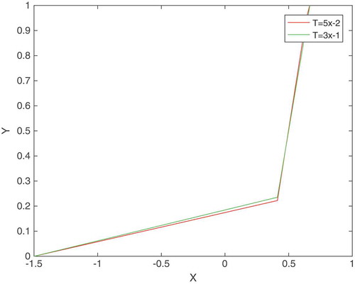
In this section, a numerical experiment is given to validate the stability of convergence of Gauss-type proximal point method.
Example 6.1. Let . Define a set-valued mapping
on
by
. Then Algorithm 5.2 generates a sequence for solving (3.1), which is converges to
.
Solution: Let us consider . It is obvious from the statement that
has a closed graph at
. From the definition of
, we have that
On the other hand, the nonemptyness of implies that
and we have, Theorem 5.1, that
Then by the definition of , we obtain that
, and hence for given values of
and
, we see that
. Thus, this implies that the sequence generated by Algorithm 5.2 converges linearly. Using Mat lab program, we present the solution of (3.1), which is
, when the number of iterations are
. Similarly, we can use the same approach for finding the solution of (3.1) when
. The Table shows the numerical results and Figure gives the graphical representation of
.
Table 1. Finding a solution of generalized equation
Figure 1. The figure for set-valued mappings .
5. Concluding remarks
When , we have established the semilocal and local convergence of the restricted proximal point method defined by Algorithm 5.2 under the assumption that
is metrically regular. Our proposed method coincides with the Gauss-type proximal point algorithm introduced by Rashid et al. in Rashid et al. (Citation2013) when
. Moreover, when
,
and the set
is singleton, the Algorithm 5.2 reduces to the classical proximal point algorithm defined by Algorithm 5.1. The convergence result established in the present article is ensuring the validity of the Gauss-type proximal point method, introduced by Rashid et al. in Rashid et al. (Citation2013), in the sense that the convergence result is uniform. Therefore, this study improves and extends the result corresponding to (Rashid et al., Citation2013). Finally, we have presented a numerical experiment that illustrated the theoretical result.
Acknowledgements
The author thanks the anonymous referees for their insightful comments and constructive suggestions, which contribute to the improvement of the initial versions of this manuscript. The author is also grateful to the associate editor for his constructive suggestions which have improved the presentation of this manuscript.
Additional information
Funding
Notes on contributors

M.H. Rashid
Mohammed Harunor Rashid is an Associate Professor in the Department of Mathematics, University of Rajshahi, Bangladesh, where he teaches calculus, geometry, real analysis, numerical analysis, vector and tensor analysis, operations research, functional analysis and other courses in both undergraduate and graduate level. Presently, he is a Postdoctoral Fellow at the Institute of Computational Mathematics and Scientific/Engineering Computing, Academy of Mathematics and Systems Science, Chinese Academy of Sciences, China. He has completed his PhD from Zhejiang University, China. His research interests focus on fuzzy Mathematics, nonlinear numerical functional analysis and nonlinear optimization, especially on generalized equations. In his investigation, he has shown how to solve generalized equations using an iterative method under some suitable conditions. He has published his research contributions in some internationally renowned journals whose publishers are Springer, Taylor & Francis, Yokohama and other journals.
References
- Alom, M. A., Rashid, M. H., & Dey, K. K. (2016). Convergence analysis of general version of Gauss-type proximal point method for metrically regular mappings. Applied Mathematics, 7(11), 1248–1259. doi:10.4236/am.2016.711110
- Anh, P. N., Muu, L. D., Nguyen, V. H., & Strodiot, J. J. (2005). Using the Banach contraction principle to implement the proximal point method for multivalued monotone variational inequalities. Journal Optim Theory Applications, 124, 285–306. doi:10.1007/s10957-004-0926-0
- Aragón Artacho, F. J., Dontchev, A. L., & Geoffroy, M. H. (2007). Convergence of the proximal point method for metrically regular mappings. ESAIM Proceedings, 17, 1–8. doi:10.1051/proc:071701
- Aragón Artacho, F. J., & Geoffroy, M. H. (2007). Uniformity and inexact version of a proximal point method for metrically regular mappings. Journal Mathematical Analysis Applications, 335, 168–183. doi:10.1016/j.jmaa.2007.01.050
- Aubin, J. P. (1984). Lipschitz behavior of solutions to convex minimization problems. Mathematical Operational Researcher, 9, 87–111. doi:10.1287/moor.9.1.87
- Aubin, J. P., & Frankowska, H. (1990). Set-valued analysis. Boston: Birkhäuser.
- Auslender, A., & Teboulle, M. (2000). Lagrangian duality and related multiplier methods for variational inequality problems. SIAM Journal Optimization, 10, 1097–1115. doi:10.1137/S1052623499352656
- Bauschke, H. H., Burke, J. V., Deutsch, F. R., Hundal, H. S., & Vanderwerff, J. (2005). D., A new proximal point iteration that converges weakly but not in norm. Proceedings Amer Mathematical Social, 133, 1829–1835. doi:10.1090/S0002-9939-05-07719-1
- Dontchev, A. L. (1996a). The Graves theorem revisited. Journal Convex Analysis, 3, 45–53.
- Dontchev, A. L. (1996b). Uniform convergence of the Newton method for Aubin continuous maps. Serdica Mathematical Journal, 22, 385–398.
- Dontchev, A. L., & Hager, W. W. (1994). An inverse mapping theorem for set-valued maps. Proceedings Amer Mathematical Social, 121, 481–498. doi:10.1090/S0002-9939-1994-1215027-7
- Dontchev, A. L., Lewis, A. S., & Rockafellar, R. T. (2002). The radius of metric regularity. Transactions AMS, 355, 493–517. doi:10.1090/S0002-9947-02-03088-X
- Dontchev, A. L., & Rockafellar, R. T. (2001). Ample parameterization of variational inclusions. SIAM Journal Optimization, 12, 170–187. doi:10.1137/S1052623400371016
- Dontchev, A. L., & Rockafellar, R. T. (2004). Regularity and conditioning of solution mappings in variational analysis. Set-Valued Anal, 12, 79–109. doi:10.1023/B:SVAN.0000023394.19482.30
- Dontchev, A. L., & Rockafellar, R. T. (2009). Implicit functions and solution mappings: A view from variational analysis. New York: Dordrecht, Heidelberg, London, LLC.
- Dontchev, A. L., & Rockafellar, R. T. (2013). Convergence of inexact Newton methods for generalized equations. Mathematical Program., Series B, 139, 115–137. doi:10.1007/s10107-013-0664-x
- Ioffe, A. D. (2000). Metric regularity and subdifferential calculus. Russian Mathematical Surveys, 55, 501–558. doi:10.1070/RM2000v055n03ABEH000292
- Ioffe, A. D., & Tikhomirov, V. M. (1979). Theory of extremal problems, studies in mathematics and its applications. Amsterdam, New York: North-Holland.
- Krasnoselskii, M. A. (1955). Two observations about the method of successive approximations. Uspekhi Matematicheskikh Nauk, 10, 123–127.
- Martinet, B. (1970). Régularisation d’inéquations variationnelles par approximations successives. Reviews French Informatics Rech Opér, 3, 154–158.
- Mordukhovich, B. S. (1992). Sensitivity analysis in nonsmooth optimization: Theoretical aspects of industrial design ( (D. A. Field and V. Komkov, eds.)). SIAM Proceedings Applications Mathematical, 58, 32–46.
- Mordukhovich, B. S. (1993). Complete characterization of opennes, metric regularity, and Lipschitzian properties of multifunctions. Transactions Amer Mathematical Social, 340(1), 1–35. doi:10.1090/S0002-9947-1993-1156300-4
- Mordukhovich, B. S. (2006). Variational analysis and generalized differentiation I: Basic theory, Grundlehren Math Wiss 330. Berlin, Heidelberg, New York: Springer-Verlag.
- Moreau, J. J. (1965). Proximité et dualité dans an espace hilbertien. Bullentin De La Societé Mathématique De France, 93, 273–299.
- Penot, J. P. (1989). Metric regularity, openness and Lipschitzian behavior of multifunctions. Nonlinear Analysis, 13, 629–643. doi:10.1016/0362-546X(89)90083-7
- Rashid, M. H., Jinhua, J. H., & Li, C. (2013). Convergence analysis of Gauss-type proximal point method for metric regular mappings. Journal Nonlinear Conv Analysis, 14(3), 627–635.
- Rashid, M. H., & Yuan, Y. X. (2017, October 20). Convergence properties of a restricted Newton-type method for generalized equations with metrically regular mappings. Applicable Analysis. 1–21. Published online. doi: 10.1080/00036811.2017.1392018
- Rockafellar, R. T. (1976a). Monotone operators and the proximal point algorithm. SIAM Journal Control Optimization, 14, 877–898. doi:10.1137/0314056
- Rockafellar, R. T. (1976b). Augmented Lagrangians and applications of the proximal point algorithm in convex programming. Mathematical Operational Researcher, 1, 97–116. doi:10.1287/moor.1.2.97
- Rockafellar, R. T., & Wets, R. J.-B. (1997). Variational analysis. Berlin: Springer-Verlag.
- Solodov, M. V., & Svaiter, B. F. (1999). A hybrid projection-proximal point algorithm. Journal Convex Analysis, 6(1), 59–70.
- Yang, Z., & He, B. (2005). A relaxed approximate proximal point algorithm. Annals Operational Researcher, 133, 119–125. doi:10.1007/s10479-004-5027-9