Multi-solitary wave solutions to the general time fractional Sharma–Tasso–Olver equation and the time fractional Cahn–Allen equation

Abstract

The space time fractional Sharma–Tasso–Olver (STO) equation and the time fractional Cahn–Allen (CA) equation are well-designated to fission and fusion phenomena including those for solitons, electromagnetic interactions, quantum relativistic atom theory, phase isolation in several components bass system, the relativistic energy-momentum relation. In this article, we have exerted the exact solution to STO and CA equation in the light of fractional derivative (e.g. modified Riemann–Liouville derivative). By using wave transformation the ODE of integer order is generated by the fractional partial differential equation (FPDE). We investigated the travelling wave solution to these equations through the recently established double$(G^{\mathrm{\text{'}}}/G,1/G)$-expansion method. The results obtained in view of hyperbolic, trigonometric and rational functions containing parameters. We have demonstrated that this method is convenient, effective and powerful tools for solving nonlinear fractional differential equations (NLFDEs).

Keywords:

• The space time fractional STO equation
• time fractional CA equation
• modified Riemann–Liouville derivative
• travelling wave solution
• solitary wave solution

MSC:

• 34C07
• 35C08
• 35K05
• 35K99
• 35P99

1. Introduction

Fractional calculus and hence fractional-order nonlinear partial differential equations have drawn the attention of many researchers for their importance to depict the inner mechanisms of the nature of real world. In the last two decades, much attention to nonlinear fractional differential equations (NLFDEs) has been inspired due to their frequent applications in the area of physics and nonlinear science. NLFDEs are well designated to many significant physical phenomena such as viscoelasticity, electromagnetism, cosmology, acoustics, plasma physics, optical fibres, solid-state physics, electrochemistry, etc. The terms diffusion, diffraction and convection are approximately correlated to the stated phenomena and are examined properly by NLFDEs. As a consequence, there has been noteworthy advancement in the study of the exact solution to NLFDEs. In the past decades, the exact solutions to NLFDEs have been studied by numerous scientists (He, 2014; Liu, Liu, Li, & He, 2017; Miller & Ross, 1993; Podlubny, 1999) who were devoted to nonlinear science and physical phenomena. They established several methods to obtain the exact solution to NLFDEs, such as the differential transformation method (Erturk, Momani, & Odibat, 2008; Wang & Wang, 2018), Adomian’s decomposition method (El-Sayed, Behiry, & Raslan, 2010), the fractional sub-equation method (Guo, Mei, Li, & Sun, 2012; Lu, 2012; Zhang & Zhang, 2011), the homotopy perturbation method (Gepreel, 2011; Gómez-Aguilar, Martinez, & Torres-Jimenez, 2017), the homotopy analysis method (Arafa, Rida, & Mohamed, 2011), the variational iteration method (Guo & Mei, 2011; Ji, Zhang, & Dong, 2012; Wang, Zhang, & Liu, 2018; Wu, 2011), the finite difference method (Seadawy, 2017b), the finite element method (Seadawy, 2017a), the exp-function method (Akbar & Ali, 2012; Bekir, Guner, & Cevikel, 2013), the improve exp(–$\varphi (\xi )$)-expansion method (Alhakim & Moussa, 2017), the $(G\mathrm{\text{'}}/G)$-expansion method and its various modifications (Akbar, Ali, & Zayed, 2012a, 2012b; Ayhan & Bekir, 2012; Batool & Ghazala, 2018; Gepreel & Omran, 2012; Islam & Akbar, 2018; Roy, Akbar, & Wazwaz, 2018; Wang, Li, & Zhang, 2008; Zhang, 2012), the first integral method (Bekir, Guner, & Unsal, 2015; Martinez, Gómez-Aguilar, & Atangana, 2018), the modified simple equation method (Akbar, Ali, & Wazwaz, 2018), the reproducing kernel method (Akgul, Baleanu, & Inc, 2016), the double$(G\mathrm{\text{'}}/G,\mathrm{ }1/G)$-expansion method (Li, Li, & Wang, 2010; Uddin, Akbar, Khan, & Haque, 2017; Zayed & Abdelaziz, 2012), etc.

Song, Wang, and Zhang (2009b) studied the analytic solutions to the Sharma–Tasso–Olver (STO) equation using various methods and made comparison with others. Rawashdeh (2015) examined the above-mentioned equation through the differential transformation method. Recently, Abdel-Salam and Hassan (2016) have studied solitary wave solutions to the suggested equation. On the other hand, Bekir, Aksoy, and Cevikel (2016) studied to find the travelling wave solutions to the Cahn–Allen (CA) equation through the sub-equation method. In addition, Esen, Yagmurlu, and Tasbozan (2013) developed the analytical solution to the mentioned equations with the homotopy analysis method. In recent years, Rawashdeh (2017) investigated the approximate solution to the suggested equations using the fractional transformation method. It is noteworthy to observe that the time fractional STO and CA equations are not examined through the recently established double $(G\mathrm{\text{'}}/G,1/G)$-expansion method. Therefore, the aim of the article is to obtain some new and further general solutions to the suggested equations through the proposed method. The mentioned method is convenient, efficient and easy to compute for investigation of the exact solutions to NLFDEs.

The general time fractional STO equation is written as: (1.1) $$D_t^{\alpha }u+3d{u}_x^2+3d{u}^2{u}_x-3du{u}_{\mathit{xx}}+d{u}_{\mathit{xxx}}=0,\mathrm{ }t>0,\mathrm{ }0<\alpha \le 1,$$(1.1) where $d$ is a nonzero constant. This equation is used to investigate the fission and fusion phenomena for solitons, quantum relativistic atom theory, electromagnetic interactions and the relativistic energy–momentum relation in mathematical physics and engineering.

The time fractional CA equation is (1.2) $$D_t^{\alpha }u-u_{\mathit{xx}}+u^3-u=0,\mathrm{ }t>0,\mathrm{ }0<\alpha \le 1.$$(1.2)

This equation is reaction diffusion equation engineering and mathematical physics which is proficient to examine the process of phase isolation in several components bass system involving order-disorder exchange.

The remaining part of the article is distributed as: In section 2 and 3, we have mentioned some definition and axioms of the Jumarie’s modified Riemann-Liouville derivative and illustrated the double $(G\mathrm{\text{'}}/G,1/G)$-expansion method, in section 4, we determine of the exact solution to the STO and CA equation due to the proposed method. In section 5, graphical representation and discussion are given. In section 6, comparison of results has been presented and in the last section, the conclusions are drawn.

2. Jumarie modified Riemann-Liouville derivative

Jumarie (2006) established the modified Riemann-Liouville derivative. First we give some principles and axioms of this type of fractional derivative which have been used our study. Suppose $f:\mathbb{R}\to \mathbb{R},$ $x\to f\left(x\right)$ be a continuous function. This derivative of order $\alpha$ is defined as: (2.1) $$D_x^{\alpha }f\left(x\right)=\left\{\begin{array}{l}\frac{1}{\mathrm{\Gamma }(-\alpha )}{\int }_0^x{(x-\xi )}^{-\alpha -1}\left[f\left(\xi \right)-f\left(0\right)\right]d\xi , \alpha <0 \\ \frac{1}{\mathrm{\Gamma }(1-\alpha )}\frac{d}{\mathit{dx}}{\int }_0^x{(x-\xi )}^{-\alpha }\left[f\left(\xi \right)-f\left(0\right)\right]d\xi ,0<\alpha <1\\ (f^{\left(n\right)}{\left(x\right))}^{\left(\alpha -n\right)}, n\le \alpha \le n+1, n\ge 1\end{array}\right.$$(2.1)

Some substantial axioms of this derivative are as: (2.2) $$D_t^{\alpha }{t}^{\gamma }=\frac{\mathrm{\Gamma }(1+\gamma )}{\mathrm{\Gamma }(1+\gamma -\alpha )}{t}^{(\gamma -\alpha )},\gamma >0$$(2.2) (2.3) $$D_t^{\alpha }\left(\mathit{af}\left(t\right)+\mathit{bg}\left(t\right)\right)=a{D}_t^{\alpha }f\left(t\right)+b{D}_t^{\alpha }g\left(t\right),$$(2.3) where $a$ and $b$ are constants, and (2.4) $$D_t^{\alpha }c=0,\mathrm{here}\mathrm{ }c\text{ is constant},$$(2.4) which are the direct results of (2.5) $$d^{\alpha }x\left(t\right)=\mathrm{\Gamma }(1+\alpha )\mathit{dx}\left(t\right).$$(2.5)

3. The double $(\mathit{G}\prime /\mathit{G},1/\mathit{G})$-expansion method

Suppose the second order ordinary differential equation (3.1) $$G^{\text{″}}\left(\xi \right)+\lambda G\left(\xi \right)=\mu ,$$(3.1)

and consider the subsequent relations (3.2) $$\varphi =G\prime /G,\psi =1/G.$$(3.2)

Thus, it provides (3.3) $${\varphi }^{\prime }=-{\varphi }^2+\mu \psi -\lambda ,{\psi }^{\prime }=-\varphi \psi .$$(3.3)

The solutions to the Equation (3.1)(3.1) $$G^{\text{″}}\left(\xi \right)+\lambda G\left(\xi \right)=\mu ,$$(3.1) depend on $\lambda$ as $\lambda <0,\lambda >0\mathrm{ }$and $\lambda =0.$

When $\lambda <0,$ the general solution to Equation (3.1)(3.1) $$G^{\text{″}}\left(\xi \right)+\lambda G\left(\xi \right)=\mu ,$$(3.1) is (3.4) $$G\left(\xi \right)=C_1\sinh \left(\sqrt{-\lambda }\mathrm{ }\xi \right)+C_2\cosh \left(\sqrt{-\lambda }\mathrm{ }\xi \right)+\frac{\mu }{\lambda }.$$(3.4)

In view of that, we attain (3.5) $${\psi }^2=\frac{-\lambda }{{\lambda }^2\sigma +{\mu }^2}({\varphi }^2-2\mu \psi +\lambda ),$$(3.5) where $\sigma =C_1^2-C_2^2.$

If $\lambda >0,$ the solution to Equation (3.1)(3.1) $$G^{\text{″}}\left(\xi \right)+\lambda G\left(\xi \right)=\mu ,$$(3.1) as follows: (3.6) $$G\left(\xi \right)=C_1\text{sin}\left(\sqrt{\lambda }\mathrm{ }\xi \right)+C_2\text{cos}\left(\sqrt{\lambda }\mathrm{ }\xi \right)+\frac{\mu }{\lambda }.$$(3.6)

As a result, we attain (3.7) $${\psi }^2=\frac{\lambda }{{\lambda }^2\sigma -{\mu }^2}({\varphi }^2-2\mu \psi +\lambda ),$$(3.7) where $\sigma =C_1^2+C_2^2.$

When $\lambda =0,$ the solution to Equation (3.1)(3.1) $$G^{\text{″}}\left(\xi \right)+\lambda G\left(\xi \right)=\mu ,$$(3.1) is: (3.8) $$G\left(\xi \right)=\frac{\mu }{2}{\xi }^2+C_1\xi +C_2.$$(3.8)

Accordingly, we attain (3.9) $${\psi }^2=\frac{1}{C_1^2-2\mu C_2}({\varphi }^2-2\mu \psi ).$$(3.9) where $C_1$and $C_2$ are arbitrary constants.

Assume that the general NLFDE of the type: (3.10) $$P\left(u,D_t^{\alpha }u,D_x^{\beta }u{,D}_t^{\alpha }{D}_t^{\alpha }u,D_t^{\alpha }{D}_x^{\beta }u,D_x^{\beta }{D}_x^{\beta },\mathrm{ }\dots \mathrm{ }\dots \mathrm{ }\dots \right)=0,0<\alpha \le 1,\mathrm{ }0<\beta \le 1,$$(3.10) here $u$ represent an unidentified function of spatial derivative $x$ and temporal derivative $t$and $P$represent a polynomial of $u(x,t)$ and its derivatives in which the maximum orderof derivatives and nonlinear terms of the maximum order are associated.

• Step 1: Consider the travelling wave transformation

(3.11) $$\xi =\frac{x^{\beta }}{\mathrm{\Gamma }(1+\beta )}+\frac{\omega t^{\alpha }}{\mathrm{\Gamma }(1+\alpha )}, u\left(x,t\right)=u(\xi ),$$(3.11)

where $\omega$ is a nonzero arbitrary constant. This transform was first proposed by He and Li (Liu et al., 2017; Wang & Wang, 2018; Wang et al., 2018).

By means of this transformation, we can write the Equation (3.10)(3.10) $$P\left(u,D_t^{\alpha }u,D_x^{\beta }u{,D}_t^{\alpha }{D}_t^{\alpha }u,D_t^{\alpha }{D}_x^{\beta }u,D_x^{\beta }{D}_x^{\beta },\mathrm{ }\dots \mathrm{ }\dots \mathrm{ }\dots \right)=0,0<\alpha \le 1,\mathrm{ }0<\beta \le 1,$$(3.10) as: (3.12) $$Q\left(u,u^{\prime },u^{\text{″}},u^{\text{″′}},\mathrm{ }\dots \mathrm{ }\dots \mathrm{ }\dots \right)=0,$$(3.12) where prime represents the differentiation with respect to $\xi .$

• Step 2: Consider the solution to Equation (3.3)(3.3) $${\varphi }^{\prime }=-{\varphi }^2+\mu \psi -\lambda ,{\psi }^{\prime }=-\varphi \psi .$$(3.3) have been revealed as a polynomial in $\varphi$ and $\psi$ of the prescribe type:

(3.13) $$u\left(\xi \right)=\sum _{i=0}^N{a}_i{\varphi }^i+\sum _{i=1}^N{b}_i{\varphi }^{i-1}\psi ,$$(3.13)

where $a_i,$$b_i$ are constants to be evaluated afterwards.

• Step 3: Balancing the maximum number of derivatives in linear and nonlinear terms appearing in Equation (3.12)(3.12) $$Q\left(u,u^{\prime },u^{\text{″}},u^{\text{″′}},\mathrm{ }\dots \mathrm{ }\dots \mathrm{ }\dots \right)=0,$$(3.12) fixed the positive integer$N$which specifies the Equation (3.13)(3.13) $$u\left(\xi \right)=\sum _{i=0}^N{a}_i{\varphi }^i+\sum _{i=1}^N{b}_i{\varphi }^{i-1}\psi ,$$(3.13) .

• Step 4: Setting (3.13)(3.13) $$u\left(\xi \right)=\sum _{i=0}^N{a}_i{\varphi }^i+\sum _{i=1}^N{b}_i{\varphi }^{i-1}\psi ,$$(3.13) into (3.12)(3.12) $$Q\left(u,u^{\prime },u^{\text{″}},u^{\text{″′}},\mathrm{ }\dots \mathrm{ }\dots \mathrm{ }\dots \right)=0,$$(3.12) together with (3.3)(3.3) $${\varphi }^{\prime }=-{\varphi }^2+\mu \psi -\lambda ,{\psi }^{\prime }=-\varphi \psi .$$(3.3) and (3.5)(3.5) $${\psi }^2=\frac{-\lambda }{{\lambda }^2\sigma +{\mu }^2}({\varphi }^2-2\mu \psi +\lambda ),$$(3.5) it reduces to a polynomial in $\varphi$ and $\psi ,$ where degree of $\psi$ is single. Comparing the polynomial of like terms to zero give an arrangement of algebraic equations that is probed by utilising computational software yields the values of $a_i{,b}_i,\mu ,C_1,C_2$ and $\lambda$ where $\lambda <0,$ which provide hyperbolic function solutions.

• Step 5: Similarly, we investigate the values of $a_i{,b}_i,\mu ,C_1,C_2$ and $\lambda$ when $\lambda >0$ and $\lambda =0,$ yield the trigonometric and rational function solutions correspondingly.

4. Determination of exact solutions

In this section, we set up some new and further general closed form travelling wave solutions to the STO and CA equation by using the double $(G\prime /G,1/G)$-expansion method.

4.1. The general time fractional STO equation

For the STO Equation (1.1)(1.1) $$D_t^{\alpha }u+3d{u}_x^2+3d{u}^2{u}_x-3du{u}_{\mathit{xx}}+d{u}_{\mathit{xxx}}=0,\mathrm{ }t>0,\mathrm{ }0<\alpha \le 1,$$(1.1) , we use the subsequent nonlinear complex wave transformation: (4.1) $$\xi =x-\frac{\omega t^{\alpha }}{\mathrm{\Gamma }\left(1+\alpha \right)}, u\left(x,t\right)=u(\xi ),$$(4.1) where in $\omega$ is a velocity of the travelling wave. Using the complex wave transformation (4.1)(4.1) $$\xi =x-\frac{\omega t^{\alpha }}{\mathrm{\Gamma }\left(1+\alpha \right)}, u\left(x,t\right)=u(\xi ),$$(4.1) , the STO equation (1.1(1.1) $$D_t^{\alpha }u+3d{u}_x^2+3d{u}^2{u}_x-3du{u}_{\mathit{xx}}+d{u}_{\mathit{xxx}}=0,\mathrm{ }t>0,\mathrm{ }0<\alpha \le 1,$$(1.1) ) transformed to the integer order ODE: (4.2) $$-\omega u^{\prime }+3d{\left(u^{\prime }\right)}^2+3d{u}^2{u}^{\prime }+3du{u}^{\text{″}}+d{u}^{\text{″′}}=0.$$(4.2)

Integrating Equation (4.2)(4.2) $$-\omega u^{\prime }+3d{\left(u^{\prime }\right)}^2+3d{u}^2{u}^{\prime }+3du{u}^{\text{″}}+d{u}^{\text{″′}}=0.$$(4.2) once and choosing a zero integrating constant, we obtain (4.3) $$-\omega u+3du{u}^{\prime }+d{u}^3+d{u}^{\text{''}}=0,$$(4.3)

Balancing the maximum-order derivative in linear and nonlinear terms provides $N=1.$ So, the solution of Equation (4.2(4.1) $$\xi =x-\frac{\omega t^{\alpha }}{\mathrm{\Gamma }\left(1+\alpha \right)}, u\left(x,t\right)=u(\xi ),$$(4.1) ) can be written in the subsequent shape: (4.4) $$u\left(\xi \right)=a_0+a_1\varphi \left(\xi \right)+b_1\psi (\xi ),$$(4.4) where $a_0,a_1,$$b_1$ are constants to be evaluated later.

Case 1:

For $\lambda <0,$ inserting Equation (4.4)(4.4) $$u\left(\xi \right)=a_0+a_1\varphi \left(\xi \right)+b_1\psi (\xi ),$$(4.4) into Equation (4.3)(4.3) $$-\omega u+3du{u}^{\prime }+d{u}^3+d{u}^{\text{''}}=0,$$(4.3) alongside Equations (3.3)(3.3) $${\varphi }^{\prime }=-{\varphi }^2+\mu \psi -\lambda ,{\psi }^{\prime }=-\varphi \psi .$$(3.3) and (3.5)(3.5) $${\psi }^2=\frac{-\lambda }{{\lambda }^2\sigma +{\mu }^2}({\varphi }^2-2\mu \psi +\lambda ),$$(3.5) and putting every coefficient to zero gives the subsequent set of mathematical equations: (4.5) $$\begin{array}{c}{\varphi }^0:d{a}_0{\mu }^4-6d{a}_0{a}_1{\lambda }^3\sigma {\mu }^2-3d{a}_0{b}_1^2{\lambda }^2{\mu }^2-3d{b}_1{\lambda }^2{a}_1{\mu }^3+d{b}_1{\lambda }^4\mu \sigma -\omega a_0{\mu }^4-3d{a}_0{a}_1{\lambda }^5{\mu }^2-3d{a}_0{a}_1\lambda {\mu }^4-3d{b}_1{\lambda }^4{a}_1\mu \sigma -2d{b}_1^3{\lambda }^3\mu +2d{a}_1^3{\mu }^2{\lambda }^2\sigma +d{a}_1^3{\lambda }^4{\sigma }^2-3d{a}_0{b}_1^2{\lambda }^4\sigma +d{b}_1{\lambda }^2{\mu }^3-2\omega a_0{\lambda }^2\sigma {\mu }^2-\omega a_0{\lambda }^4{\sigma }^2=0\\ {\varphi }^1:4d{a}_1{\lambda }^3\sigma {\mu }^2+3d{a}_0^2{a}_1{\mu }^4-\omega a_1{\lambda }^4{\sigma }^2+2d{a}_1\lambda {\mu }^4+2d{a}_1{\lambda }^5{\sigma }^2+6d{a}_0^2{a}_1{\lambda }^2\sigma {\mu }^2-3d{a}_1^2{\lambda }^5{\sigma }^2-6d{a}_1^2{\lambda }^3{\mu }^2\sigma +3d{b}_1^2{\lambda }^4\sigma +3d{b}_1^2{\lambda }^2{\mu }^2-3d{a}_1^2\lambda {\mu }^4-\omega a_1{\mu }^4+3d{a}_0^2{a}_1{\lambda }^4{\sigma }^2-3d{a}_1{b}_1^2{\lambda }^2{\mu }^2-2\omega a_1{\mu }^2{\lambda }^2\sigma -3d{a}_1{b}_1^2{\lambda }^4\sigma =0\\ {\varphi }^2:-3d{b}_1{\lambda }^3{a}_1\mu \sigma +3d{a}_0{a}_1^2{\lambda }^4{\sigma }^2+d{b}_1\lambda {\mu }^3-6d{a}_0{a}_1{\lambda }^2\sigma {\mu }^2-3d{a}_0{b}_1^2\lambda {\mu }^2-3d{a}_0{a}_1{\mu }^4-3d{b}_1\lambda a_1{\mu }^3+d{b}_1{\lambda }^3\mu \sigma -2d{b}_1^3{\lambda }^2\mu +6d{a}_0{a}_1^2{\lambda }^2\sigma {\mu }^2-3d{a}_0{a}_1{\lambda }^4{\sigma }^2-3d{a}_0{b}_1^2{\lambda }^2\sigma +3d{a}_0{a}_1^2{\mu }^4=0\end{array}$$(4.5) $${\varphi }^3:2d{a}_1{\lambda }^4{\sigma }^2+d{a}_1^3{\mu }^4-3d{a}_1^2{\mu }^4+4d{a}_1{\mu }^2{\lambda }^2\sigma +d{a}_1^3{\lambda }^4{\sigma }^2+2d{a}_1{\mu }^4+3d{b}_1^2\lambda {\mu }^2-3d{a}_1^2{\lambda }^4{\sigma }^2+2d{a}_1^3{\mu }^2{\lambda }^2\sigma -3d{a}_1{b}_1^2{\lambda }^3\sigma -3d{a}_1{b}_1^2\lambda {\mu }^2-6d{a}_1^2{\mu }^2{\lambda }^2\sigma +3d{b}_1^2{\lambda }^3\sigma =\mathrm{ }0$$ $$\psi :-d{b}_1^3{\lambda }^4\sigma -\omega b_1{\mu }^4+3d{a}_0^2{b}_1{\lambda }^4{\sigma }^2+d{b}_1{\lambda }^5{\sigma }^2-3d{b}_1{a}_1{\lambda }^5{\sigma }^2-d{b}_1\lambda {\mu }^4+\mathrm{ }3d{a}_0^2{b}_1{\mu }^4+3d{b}_1\lambda a_1{\mu }^4+6d{a}_0{b}_1^2{\lambda }^3\mu \sigma +3d{a}_0{a}_1\mu {\lambda }^4{\sigma }^2+3d{b}_1^3{\lambda }^2{\mu }^2+6d{a}_0^2{b}_1{\lambda }^2\sigma {\mu }^2-2\omega b_1{\mu }^2{\lambda }^2\sigma -\omega b_1{\lambda }^4{\sigma }^2+6d{a}_0{b}_1^2\lambda {\mu }^3+3d{a}_0{a}_1{\mu }^5+\mathrm{ }6d{a}_0{a}_1{\mu }^3{\lambda }^2\sigma =0$$ $$\varphi \psi :-6d{b}_1^2{\lambda }^3\mu \sigma +6d{a}_0{a}_1{b}_1{\lambda }^4{\sigma }^2+6d{a}_1{b}_1^2\lambda {\mu }^3+12d{a}_0{a}_1{b}_1{\lambda }^2\sigma {\mu }^2+3d{a}_1^2{\mu }^5-\mathrm{ }6d{b}_1^2\lambda {\mu }^3-6d{a}_0{b}_1{\mu }^2{\lambda }^2\sigma +6d{a}_1{b}_1^2\lambda \mu \sigma -3d{a}_1\mu {\lambda }^4{\sigma }^2-3d{a}_1{\mu }^5-\mathrm{ }3d{a}_1{b}_1{\lambda }^4{\sigma }^2-3d{a}_0{b}_1{\mu }^4+6d{a}_1^2{\mu }^3{\lambda }^2\sigma +6d{a}_0{a}_1{b}_1{\mu }^4+3d{a}_1^2\mu {\lambda }^4{\sigma }^2-\mathrm{ }6d{a}_1{\mu }^3{\lambda }^2\sigma =0$$ $${\varphi }^2\psi :4d{b}_1{\lambda }^2\sigma {\mu }^2+3d{a}_1^2{b}_1{\lambda }^4{\sigma }^2+3d{a}_1^2{b}_1{\mu }^4-6d{a}_1{b}_1{\mu }^4+6d{a}_1^2{b}_1{\mu }^2{\lambda }^2\sigma +\mathrm{ }2d{b}_1{\mu }^4-d{b}_1^3\lambda {\mu }^2-d{b}_1^3{\lambda }^3\sigma -12d{a}_1{b}_1{\mu }^2{\lambda }^2\sigma -6d{a}_1{b}_1{\lambda }^4{\sigma }^2+2d{b}_1{\lambda }^4{\sigma }^2=0.$$

Solving the mathematical Equation (4.5)(4.5) $$\begin{array}{c}{\varphi }^0:d{a}_0{\mu }^4-6d{a}_0{a}_1{\lambda }^3\sigma {\mu }^2-3d{a}_0{b}_1^2{\lambda }^2{\mu }^2-3d{b}_1{\lambda }^2{a}_1{\mu }^3+d{b}_1{\lambda }^4\mu \sigma -\omega a_0{\mu }^4-3d{a}_0{a}_1{\lambda }^5{\mu }^2-3d{a}_0{a}_1\lambda {\mu }^4-3d{b}_1{\lambda }^4{a}_1\mu \sigma -2d{b}_1^3{\lambda }^3\mu +2d{a}_1^3{\mu }^2{\lambda }^2\sigma +d{a}_1^3{\lambda }^4{\sigma }^2-3d{a}_0{b}_1^2{\lambda }^4\sigma +d{b}_1{\lambda }^2{\mu }^3-2\omega a_0{\lambda }^2\sigma {\mu }^2-\omega a_0{\lambda }^4{\sigma }^2=0\\ {\varphi }^1:4d{a}_1{\lambda }^3\sigma {\mu }^2+3d{a}_0^2{a}_1{\mu }^4-\omega a_1{\lambda }^4{\sigma }^2+2d{a}_1\lambda {\mu }^4+2d{a}_1{\lambda }^5{\sigma }^2+6d{a}_0^2{a}_1{\lambda }^2\sigma {\mu }^2-3d{a}_1^2{\lambda }^5{\sigma }^2-6d{a}_1^2{\lambda }^3{\mu }^2\sigma +3d{b}_1^2{\lambda }^4\sigma +3d{b}_1^2{\lambda }^2{\mu }^2-3d{a}_1^2\lambda {\mu }^4-\omega a_1{\mu }^4+3d{a}_0^2{a}_1{\lambda }^4{\sigma }^2-3d{a}_1{b}_1^2{\lambda }^2{\mu }^2-2\omega a_1{\mu }^2{\lambda }^2\sigma -3d{a}_1{b}_1^2{\lambda }^4\sigma =0\\ {\varphi }^2:-3d{b}_1{\lambda }^3{a}_1\mu \sigma +3d{a}_0{a}_1^2{\lambda }^4{\sigma }^2+d{b}_1\lambda {\mu }^3-6d{a}_0{a}_1{\lambda }^2\sigma {\mu }^2-3d{a}_0{b}_1^2\lambda {\mu }^2-3d{a}_0{a}_1{\mu }^4-3d{b}_1\lambda a_1{\mu }^3+d{b}_1{\lambda }^3\mu \sigma -2d{b}_1^3{\lambda }^2\mu +6d{a}_0{a}_1^2{\lambda }^2\sigma {\mu }^2-3d{a}_0{a}_1{\lambda }^4{\sigma }^2-3d{a}_0{b}_1^2{\lambda }^2\sigma +3d{a}_0{a}_1^2{\mu }^4=0\end{array}$$(4.5) using computer algebra such as Maple, we achieve the given solutions:

• Set 1: $a_0=0,$$a_1=\frac{1}{2},$ $b_1=\pm \sqrt{\frac{-{\mu }^2-{\lambda }^2\sigma }{4\lambda }}$ and $\omega =-\frac{d\lambda }{4}.$

• Set 2: $a_0=\frac{\sqrt{-\lambda }}{2},$ $a_1=\frac{1}{2},$ $b_1=\pm \sqrt{\frac{-{\mu }^2-{\lambda }^2\sigma }{4\lambda }}$ and $\omega =-d\lambda .$

• Set 3: $a_0=0,$ $a_1=1,$ $b_1=\pm \sqrt{\frac{-{\mu }^2-{\lambda }^2\sigma }{\lambda }}$ and $\omega =-d\lambda .$

Now we obtain the following exact solution to the STO equation for set 1: (4.6) $$\begin{array}{c}{u}_{1_1}\left(x,t\right)=\frac{1}{2}\times \frac{C_1.\sqrt{-\lambda }\cosh \left(\sqrt{-\lambda }\xi \right)+C_2.\sqrt{-\lambda }\sinh \left(\sqrt{-\lambda }\xi \right)}{C_1\sinh \left(\sqrt{-\lambda }\xi \right)+C_2\cosh \left(\sqrt{-\lambda }\xi \right)+\frac{\mu }{\lambda }}\\ \pm \sqrt{\frac{-{\mu }^2-{\lambda }^2\sigma }{4\lambda }}\times \frac{1}{C_1\sinh \left(\sqrt{-\lambda }\xi \right)+C_2\cosh \left(\sqrt{-\lambda }\xi \right)+\frac{\mu }{\lambda }},\end{array}$$(4.6) where $\sigma =C_1^2-C_2^2$ and $\xi =x+\frac{\frac{d\lambda }{4}{t}^{\alpha }}{\mathrm{\Gamma }(1+\alpha )}.$

As $C_1$ and $C_2$ are integral constants, it might be arbitrarily chosen. If we choose $C_1=0,$ $C_2\ne 0$ and $\mu =0$ in Equation (4.6(4.1) $$\xi =x-\frac{\omega t^{\alpha }}{\mathrm{\Gamma }\left(1+\alpha \right)}, u\left(x,t\right)=u(\xi ),$$(4.1) ), we find the solitary wave solution (4.7) $$u_{1_2}\left(x,t\right)=\frac{\sqrt{-\lambda }}{2}\times \tanh \left(\sqrt{-\lambda }(x+\frac{\frac{d\lambda }{4}{t}^{\alpha }}{\mathrm{\Gamma }\left(1+\alpha \right)})\right)\pm \frac{\sqrt{-\lambda \sigma }}{2}\times \mathit{sech}\left(\sqrt{-\lambda }\right(x+\frac{\frac{d\lambda }{4}{t}^{\alpha }}{\mathrm{\Gamma }\left(1+\alpha \right)}\left)\right).$$(4.7)

Again, if we set $C_1\ne 0,$ $C_2=0$ and $\mu =0$ in Equation (4.6)(4.6) $$\begin{array}{c}{u}_{1_1}\left(x,t\right)=\frac{1}{2}\times \frac{C_1.\sqrt{-\lambda }\cosh \left(\sqrt{-\lambda }\xi \right)+C_2.\sqrt{-\lambda }\sinh \left(\sqrt{-\lambda }\xi \right)}{C_1\sinh \left(\sqrt{-\lambda }\xi \right)+C_2\cosh \left(\sqrt{-\lambda }\xi \right)+\frac{\mu }{\lambda }}\\ \pm \sqrt{\frac{-{\mu }^2-{\lambda }^2\sigma }{4\lambda }}\times \frac{1}{C_1\sinh \left(\sqrt{-\lambda }\xi \right)+C_2\cosh \left(\sqrt{-\lambda }\xi \right)+\frac{\mu }{\lambda }},\end{array}$$(4.6) , we obtain the solitary wave solution (4.8) $$u_{1_3}\left(x,t\right)=\frac{\sqrt{-\lambda }}{2}\times \coth \left(\sqrt{-\lambda }(x+\frac{\frac{d\lambda }{4}{t}^{\alpha }}{\mathrm{\Gamma }\left(1+\alpha \right)})\right)\pm \frac{\sqrt{-\lambda \sigma }}{2}\times \mathit{cosech}\left(\sqrt{-\lambda }\right(x+\frac{\frac{d\lambda }{4}{t}^{\alpha }}{\mathrm{\Gamma }\left(1+\alpha \right)}\left)\right).$$(4.8)

Case 2:

In a similar manner, when $\lambda >0,$ inserting Equation (4.4)(4.4) $$u\left(\xi \right)=a_0+a_1\varphi \left(\xi \right)+b_1\psi (\xi ),$$(4.4) into Equation (4.3)(4.3) $$-\omega u+3du{u}^{\prime }+d{u}^3+d{u}^{\text{''}}=0,$$(4.3) along with Equations (3.3)(3.3) $${\varphi }^{\prime }=-{\varphi }^2+\mu \psi -\lambda ,{\psi }^{\prime }=-\varphi \psi .$$(3.3) and (3.7)(3.7) $${\psi }^2=\frac{\lambda }{{\lambda }^2\sigma -{\mu }^2}({\varphi }^2-2\mu \psi +\lambda ),$$(3.7) delivers a cluster of mathematical equations for $a_0,a_1,$ $b_1$ and $\omega$ and solving these equations, we attain the following results:

• Set 1: $a_0=0,$ $a_1=\frac{1}{2},$ $b_1=\pm \sqrt{\frac{-{\mu }^2+{\lambda }^2\sigma }{4\lambda }}$ and $\omega =-\frac{d\lambda }{4}.$

• Set 2: $a_0=\frac{\sqrt{-\lambda }}{2},$ $a_1=\frac{1}{2},$ $b_1=\pm \sqrt{\frac{-{\mu }^2+{\lambda }^2\sigma }{4\lambda }}$ and $\omega =-d\lambda .$

• Set 3: $a_0=0,$ $a_1=1,$ $b_1=\pm \sqrt{\frac{-{\mu }^2+{\lambda }^2\sigma }{\lambda }}$ and $\omega =-d\lambda .$

Substituting the results of set 1 in Equation (4.4)(4.4) $$u\left(\xi \right)=a_0+a_1\varphi \left(\xi \right)+b_1\psi (\xi ),$$(4.4) attains the solution of Equation (1.1)(1.1) $$D_t^{\alpha }u+3d{u}_x^2+3d{u}^2{u}_x-3du{u}_{\mathit{xx}}+d{u}_{\mathit{xxx}}=0,\mathrm{ }t>0,\mathrm{ }0<\alpha \le 1,$$(1.1) : (4.9) $$u_{1_4}\left(x,t\right)=\frac{1}{2}\times \frac{C_1.\sqrt{\lambda }\text{cos}\left(\sqrt{\lambda }\xi \right)-C_2.\sqrt{\lambda }\text{sin}\left(\sqrt{\lambda }\xi \right)}{C_1\text{sin}\left(\sqrt{\lambda }\xi \right)+C_2\text{cos}\left(\sqrt{\lambda }\xi \right)+\frac{\mu }{\lambda }}\pm \sqrt{\frac{-{\mu }^2+{\lambda }^2\sigma }{4\lambda }}\frac{1}{C_1\text{sin}\left(\sqrt{\lambda }\xi \right)+C_2\text{cos}\left(\sqrt{\lambda }\xi \right)+\frac{\mu }{\lambda }},$$(4.9) where $\sigma =C_1^2+C_2^2$ and $\xi =x+\frac{\frac{d\lambda }{4}{t}^{\alpha }}{\mathrm{\Gamma }\left(1+\alpha \right)}.$

If $C_1=0,$ $C_2\ne 0$(or $C_1\ne 0,$ $C_2=0$) and $\mu =0$ then from Equation (4.9)(4.9) $$u_{1_4}\left(x,t\right)=\frac{1}{2}\times \frac{C_1.\sqrt{\lambda }\text{cos}\left(\sqrt{\lambda }\xi \right)-C_2.\sqrt{\lambda }\text{sin}\left(\sqrt{\lambda }\xi \right)}{C_1\text{sin}\left(\sqrt{\lambda }\xi \right)+C_2\text{cos}\left(\sqrt{\lambda }\xi \right)+\frac{\mu }{\lambda }}\pm \sqrt{\frac{-{\mu }^2+{\lambda }^2\sigma }{4\lambda }}\frac{1}{C_1\text{sin}\left(\sqrt{\lambda }\xi \right)+C_2\text{cos}\left(\sqrt{\lambda }\xi \right)+\frac{\mu }{\lambda }},$$(4.9) , we obtain the solitary wave solution (4.10) $$u_{1_5}\left(x,t\right)=\frac{\sqrt{\lambda }}{2}\times \text{tan}\left(\sqrt{\lambda }(x+\frac{\frac{d\lambda }{4}{t}^{\alpha }}{\mathrm{\Gamma }\left(1+\alpha \right)})\right)\pm \frac{\sqrt{\lambda \sigma }}{2}\times \text{sec}\left(\sqrt{\lambda }\right(x+\frac{\frac{d\lambda }{4}{t}^{\alpha }}{\mathrm{\Gamma }\left(1+\alpha \right)}\left)\right).$$(4.10) (4.11) $$u_{1_6}\left(x,t\right)=\frac{\sqrt{\lambda }}{2}\times \text{cot}\left(\sqrt{\lambda }(x+\frac{\frac{d\lambda }{4}{t}^{\alpha }}{\mathrm{\Gamma }\left(1+\alpha \right)})\right)\pm \frac{\sqrt{\lambda \sigma }}{2}\times \text{cosec}\left(\sqrt{\lambda }\right(x+\frac{\frac{d\lambda }{4}{t}^{\alpha }}{\mathrm{\Gamma }\left(1+\alpha \right)}\left)\right).$$(4.11)

Case 3:

In a similar fashion, when $\lambda =0,$ by using Equations (4.4)(4.4) $$u\left(\xi \right)=a_0+a_1\varphi \left(\xi \right)+b_1\psi (\xi ),$$(4.4) and (4.3)(4.3) $$-\omega u+3du{u}^{\prime }+d{u}^3+d{u}^{\text{''}}=0,$$(4.3) along with Equations (3.3)(3.3) $${\varphi }^{\prime }=-{\varphi }^2+\mu \psi -\lambda ,{\psi }^{\prime }=-\varphi \psi .$$(3.3) and (3.9)(3.9) $${\psi }^2=\frac{1}{C_1^2-2\mu C_2}({\varphi }^2-2\mu \psi ).$$(3.9) , we find a cluster of algebraic equations whose solutions are as follows:

• Set 1: $a_0=0,$ $a_1=1,$ $b_1=\pm \sqrt{C_1^2-2\mu C_2},$ and $\omega =0.$

• Set 2: $a_0=0,$ $a_1=\frac{1}{2},$ $b_1=\pm \sqrt{C_1^2-2\mu C_2},$ and $\omega =0.$

Inserting the value scheduled in set 1 into Equation (4.4(4.1) $$\xi =x-\frac{\omega t^{\alpha }}{\mathrm{\Gamma }\left(1+\alpha \right)}, u\left(x,t\right)=u(\xi ),$$(4.1) ), we achieve the subsequent solution of Equation (4.2)(4.2) $$-\omega u^{\prime }+3d{\left(u^{\prime }\right)}^2+3d{u}^2{u}^{\prime }+3du{u}^{\text{″}}+d{u}^{\text{″′}}=0.$$(4.2) (4.12) $$u_{1_7}\left(x,t\right)=\frac{\mu \xi +C_1}{\frac{\mu }{2}{\xi }^2+C_1\xi +C_2}\pm \sqrt{C_1^2-2\mu C_2}\times \frac{1}{\frac{\mu }{2}{\xi }^2+C_1\xi +C_2},$$(4.12) where $\xi =x-\frac{\omega t^{\alpha }}{\mathrm{\Gamma }(1+\alpha )}.$

It can be mentioned that the solution $u_{1_1}$-$u_{1_7}$of the general time fractional STO equation is new and further general and is not examined in earlier works. These solutions are convenient to investigate the fission and fusion phenomena theoretically in mathematical physics and engineering.

It is noteworthy to observe that for the results of the constants given in set 2 and set 3 (both in case 1 and case 2) and set 2 for case 3, we attain fresh and more general solitary wave solutions which also useful to analysis the fission and fusion phenomena. For simplicity the solutions are omitted here.

4.2. The fractional CA equation

In this subsection, we have investigated the more general and some fresh solutions to the fractional CA Equation (1.2)(1.2) $$D_t^{\alpha }u-u_{\mathit{xx}}+u^3-u=0,\mathrm{ }t>0,\mathrm{ }0<\alpha \le 1.$$(1.2) via the double $(G\prime /G,1/G)$-expansion method. For the mentioned equation, introducing the subsequent transformation: (4.13) $$\xi =\mathit{kx}-\frac{c{t}^{\alpha }}{\mathrm{\Gamma }\left(1+\alpha \right)}, u\left(x,t\right)=u(\xi ),$$(4.13) where $c$ is the velocity of the travelling wave. Using Equation (4.13(4.1) $$\xi =x-\frac{\omega t^{\alpha }}{\mathrm{\Gamma }\left(1+\alpha \right)}, u\left(x,t\right)=u(\xi ),$$(4.1) ) into Equation (1.2)(1.2) $$D_t^{\alpha }u-u_{\mathit{xx}}+u^3-u=0,\mathrm{ }t>0,\mathrm{ }0<\alpha \le 1.$$(1.2) transformed to the following ODE for $u=u(\xi ):$ (4.14) $$-c{u}^{\prime }-k^2{u}^{\text{″}}+u^3-u=0.$$(4.14)

Balancing the maximum order derivative and nonlinear term provides $N=1.$ Therefore, the solution of Equation (1.2)(1.2) $$D_t^{\alpha }u-u_{\mathit{xx}}+u^3-u=0,\mathrm{ }t>0,\mathrm{ }0<\alpha \le 1.$$(1.2) is of the form: (4.15) $$u\left(\xi \right)=a_0+a_1\varphi \left(\xi \right)+b_1\psi (\xi ).$$(4.15)

Case 1:

For $\lambda <0,$ inserting Equation (4.15)(4.15) $$u\left(\xi \right)=a_0+a_1\varphi \left(\xi \right)+b_1\psi (\xi ).$$(4.15) into Equation (4.14)(4.14) $$-c{u}^{\prime }-k^2{u}^{\text{″}}+u^3-u=0.$$(4.14) with Equations (3.3)(3.3) $${\varphi }^{\prime }=-{\varphi }^2+\mu \psi -\lambda ,{\psi }^{\prime }=-\varphi \psi .$$(3.3) and (3.5)(3.5) $${\psi }^2=\frac{-\lambda }{{\lambda }^2\sigma +{\mu }^2}({\varphi }^2-2\mu \psi +\lambda ),$$(3.5) provides a system of mathematical equations as follows: (4.16) $$\begin{array}{c}{\varphi }^0:2a_0{\lambda }^2\sigma {\mu }^2-c{a}_1{\lambda }^5{\sigma }^2-c{a}_1\lambda {\mu }^4+k^2{b}_1{\lambda }^2{\mu }^3-2c{a}_1{\lambda }^3\sigma {\mu }^2+k^2{b}_1{\lambda }^4\mu \sigma -a_0^3{\mu }^4-a_0^3{\lambda }^4{\sigma }^2+a_0{\lambda }^4{\sigma }^2+2b_1^3{\lambda }^3\mu -2a_0^3{\lambda }^2\sigma {\mu }^2+3a_0{b}_1^2{\lambda }^4\sigma +3a_0{b}_1^2{\lambda }^2{\mu }^2+a_0{\mu }^4=0\\ {\varphi }^1:4k^2{a}_1{\lambda }^3\sigma {\mu }^2+2a_1{\mu }^2{\lambda }^2\sigma +a_1{\lambda }^4{\sigma }^2+3a_1{b}_1^2{\lambda }^2{\mu }^2-3a_0^2{a}_1{\mu }^4-3a_0^2{a}_1{\lambda }^4{\sigma }^2+2k^2{a}_1\lambda {\mu }^4+a_1{\mu }^4+2k^2{a}_1{\lambda }^5{\sigma }^2-6a_0^2{a}_1{\lambda }^2\sigma {\mu }^2+3a_1{b}_1^2{\lambda }^4\sigma =0\\ {\varphi }^2:-c{a}_1{\lambda }^4{\sigma }^2+3a_0{b}_1^2\lambda {\mu }^2+k^2{b}_1\lambda {\mu }^3-3a_0{a}_1^2{\lambda }^4{\sigma }^2+3a_0{b}_1^2{\lambda }^3\sigma +2b_1^3{\lambda }^2\mu -c{a}_1{\mu }^4+k^2{b}_1{\lambda }^3\mu \sigma -6a_0{a}_1^2{\lambda }^2\sigma {\mu }^2-3a_0{a}_1^2{\mu }^4-2c{a}_1{\lambda }^2\sigma {\mu }^2=0\\ {\varphi }^3:-2a_1^3{\mu }^2{\lambda }^2\sigma +3a_1{b}_1^2{\lambda }^3\sigma -a_1{\mu }^4+3a_1{b}_1^2\lambda {\mu }^2+2k^2{a}_1{\lambda }^4{\sigma }^2-a_1^3{\lambda }^4{\sigma }^2+2k^2{a}_1{\mu }^4+4k^2{a}_1{\lambda }^2\sigma {\mu }^2=0\end{array}$$(4.16) $$\psi :-3a_0^2{b}_1{\lambda }^4{\sigma }^2-3a_0^2{b}_1{\mu }^4+k^2{b}_1{\lambda }^5{\sigma }^2-k^2{b}_1\lambda {\mu }^4+2b_1{\mu }^2{\lambda }^2\sigma +b_1{\lambda }^4{\sigma }^2+b_1^3{\lambda }^4\sigma -\mathrm{ }6a_0{b}_1^2\lambda {\mu }^3-6a_0{b}_1^2{\lambda }^3\mu \sigma +b_1{\mu }^4+c{a}_1\mu {\lambda }^4{\sigma }^2-3b_1^3{\lambda }^2{\mu }^2+c{a}_1{\mu }^5+2c{a}_1{\mu }^3{\lambda }^2\sigma -\mathrm{ }6a_0^2{b}_1{\lambda }^2\sigma {\mu }^2=0$$ $$\varphi \psi :-2c{b}_1{\lambda }^2\sigma {\mu }^2-6a_1{b}_1^2\lambda {\mu }^3-6a_0{a}_1{b}_1{\mu }^4-6a_0{a}_1{b}_1{\lambda }^4{\sigma }^2-6k^2{a}_1{\mu }^3{\lambda }^2\sigma -\mathrm{ }c{b}_1{\mu }^4-3k^2{a}_1\mu {\lambda }^4{\sigma }^2-3k^2{a}_1{\mu }^5-12a_0{a}_1{b}_1{\mu }^2{\lambda }^2\sigma -6a_1{b}_1^2{\lambda }^3\mu \sigma -c{b}_1{\lambda }^4{\sigma }^2=0$$ $${\varphi }^2\psi :b_1^3{\lambda }^3\sigma +2k^2{b}_1{\lambda }^4{\sigma }^2+2k^2{b}_1{\mu }^4+4k^2{b}_1{\lambda }^2\sigma {\mu }^2-6a_1^2{b}_1{\lambda }^2\sigma {\mu }^2-3a_1^2{b}_1{\mu }^4-3a_1^2{b}_1{\lambda }^4{\sigma }^2+b_1^2\lambda {\mu }^2=0.$$

Solving the algebraic Equation (4.16)(4.16) $$\begin{array}{c}{\varphi }^0:2a_0{\lambda }^2\sigma {\mu }^2-c{a}_1{\lambda }^5{\sigma }^2-c{a}_1\lambda {\mu }^4+k^2{b}_1{\lambda }^2{\mu }^3-2c{a}_1{\lambda }^3\sigma {\mu }^2+k^2{b}_1{\lambda }^4\mu \sigma -a_0^3{\mu }^4-a_0^3{\lambda }^4{\sigma }^2+a_0{\lambda }^4{\sigma }^2+2b_1^3{\lambda }^3\mu -2a_0^3{\lambda }^2\sigma {\mu }^2+3a_0{b}_1^2{\lambda }^4\sigma +3a_0{b}_1^2{\lambda }^2{\mu }^2+a_0{\mu }^4=0\\ {\varphi }^1:4k^2{a}_1{\lambda }^3\sigma {\mu }^2+2a_1{\mu }^2{\lambda }^2\sigma +a_1{\lambda }^4{\sigma }^2+3a_1{b}_1^2{\lambda }^2{\mu }^2-3a_0^2{a}_1{\mu }^4-3a_0^2{a}_1{\lambda }^4{\sigma }^2+2k^2{a}_1\lambda {\mu }^4+a_1{\mu }^4+2k^2{a}_1{\lambda }^5{\sigma }^2-6a_0^2{a}_1{\lambda }^2\sigma {\mu }^2+3a_1{b}_1^2{\lambda }^4\sigma =0\\ {\varphi }^2:-c{a}_1{\lambda }^4{\sigma }^2+3a_0{b}_1^2\lambda {\mu }^2+k^2{b}_1\lambda {\mu }^3-3a_0{a}_1^2{\lambda }^4{\sigma }^2+3a_0{b}_1^2{\lambda }^3\sigma +2b_1^3{\lambda }^2\mu -c{a}_1{\mu }^4+k^2{b}_1{\lambda }^3\mu \sigma -6a_0{a}_1^2{\lambda }^2\sigma {\mu }^2-3a_0{a}_1^2{\mu }^4-2c{a}_1{\lambda }^2\sigma {\mu }^2=0\\ {\varphi }^3:-2a_1^3{\mu }^2{\lambda }^2\sigma +3a_1{b}_1^2{\lambda }^3\sigma -a_1{\mu }^4+3a_1{b}_1^2\lambda {\mu }^2+2k^2{a}_1{\lambda }^4{\sigma }^2-a_1^3{\lambda }^4{\sigma }^2+2k^2{a}_1{\mu }^4+4k^2{a}_1{\lambda }^2\sigma {\mu }^2=0\end{array}$$(4.16) with the help of computer algebra such as Maple, we attain the given results:

• Set 1: $a_0=\frac{1}{2},$ $a_1=\pm \sqrt{-\frac{1}{4\lambda }},$ $b_1=\pm \frac{\sqrt{{\mu }^2+{\lambda }^2\sigma }}{2\lambda },$ $c=\pm 3\mathrm{ }\sqrt{-\frac{1}{4\lambda }}$ and $k=\pm \mathrm{ }\sqrt{-\frac{1}{2\lambda }}$ .

• Set 2: $a_0=-\frac{1}{2},$ $a_1=\pm \sqrt{-\frac{1}{4\lambda }},$ $b_1=\pm \frac{\sqrt{{\mu }^2+{\lambda }^2\sigma }}{2\lambda },$ $c=\pm 3\mathrm{ }\sqrt{-\frac{1}{4\lambda }}$ and $k=\pm \mathrm{ }\sqrt{-\frac{1}{2\lambda }}$ .

• Set 3: $a_0=0,$ $a_1=\pm \sqrt{-\frac{1}{\lambda }},$ $b_1=\pm \frac{\sqrt{{\mu }^2+{\lambda }^2\sigma }}{\lambda },$ $c=0\mathrm{ }$and $k=\pm \mathrm{ }\sqrt{-\frac{2}{\lambda }}$ .

Now we attain the solution of the fractional CA equation for set 1 (4.17) $$u_{2_1}\left(x,t\right)=\frac{1}{2}\pm \sqrt{-\frac{1}{4\lambda }}\times \frac{C_1.\sqrt{-\lambda }\cosh \left(\sqrt{-\lambda }\xi \right)+C_2.\sqrt{-\lambda }\sinh \left(\sqrt{-\lambda }\xi \right)}{C_1\sinh \left(\sqrt{-\lambda }\xi \right)+C_2\cosh \left(\sqrt{-\lambda }\xi \right)+\frac{\mu }{\lambda }}\mathrm{ }\pm \frac{\sqrt{{\mu }^2+{\lambda }^2\sigma }}{2\lambda }\times \frac{1}{C_1\sinh \left(\sqrt{-\lambda }\xi \right)+C_2\cosh \left(\sqrt{-\lambda }\xi \right)+\frac{\mu }{\lambda }},$$(4.17)

where$\mathrm{ }\sigma =C_1^2-C_2^2$ and $\xi =\pm \mathrm{ }\sqrt{-\frac{1}{2\lambda }}x-\frac{3\mathrm{ }\sqrt{-\frac{1}{4\lambda }}{t}^{\alpha }}{\mathrm{\Gamma }(1+\alpha )}.$

Setting $C_1=0,$ $C_2\ne 0$(or $C_1\ne 0,C_2=0$) and $\mu =0$ into Equation (4.17(4.1) $$\xi =x-\frac{\omega t^{\alpha }}{\mathrm{\Gamma }\left(1+\alpha \right)}, u\left(x,t\right)=u(\xi ),$$(4.1) ), we attain the solitary wave solution (4.18) $$u_{2_2}\left(x,t\right)=\frac{1}{2}\pm \frac{1}{2}\times \tanh \left(\sqrt{-\lambda }\xi \right)\pm \mathrm{ }\times \frac{\sqrt{\lambda \sigma }}{2}s\mathit{ech}(\sqrt{-\lambda }\xi ),$$(4.18) (4.19) $$u_{2_3}\left(x,t\right)=\frac{1}{2}\pm \frac{1}{2}\times \coth \left(\sqrt{-\lambda }\xi \right)\pm \frac{\sqrt{\lambda \sigma }}{2}\mathrm{ }\times \mathit{cosech}(\sqrt{-\lambda }\xi ),$$(4.19) where $\xi =\pm \mathrm{ }\sqrt{-\frac{1}{2\lambda }}x-\frac{3\mathrm{ }\sqrt{-\frac{1}{4\lambda }}{t}^{\alpha }}{\mathrm{\Gamma }(1+\alpha )}.$

Case 2:

In the similar approach, when $\lambda >0$ inserting Equation (4.15)(4.15) $$u\left(\xi \right)=a_0+a_1\varphi \left(\xi \right)+b_1\psi (\xi ).$$(4.15) into Equation (4.14)(4.14) $$-c{u}^{\prime }-k^2{u}^{\text{″}}+u^3-u=0.$$(4.14) along with Equations (3.3)(3.3) $${\varphi }^{\prime }=-{\varphi }^2+\mu \psi -\lambda ,{\psi }^{\prime }=-\varphi \psi .$$(3.3) and (3.7)(3.7) $${\psi }^2=\frac{\lambda }{{\lambda }^2\sigma -{\mu }^2}({\varphi }^2-2\mu \psi +\lambda ),$$(3.7) produces a collection of mathematical equations for $a_0,\mathrm{ }{a}_1,\mathrm{ }{b}_1,\mathrm{ }c,\mathrm{ }k$ and solving these equations we find the following solutions:

• Set 1: $a_0=\frac{1}{2},$ $a_1=\pm \sqrt{-\frac{1}{4\lambda }},$ $b_1=\pm \frac{\sqrt{{\mu }^2-{\lambda }^2\sigma }}{2\lambda },$ $c=\pm 3\mathrm{ }\sqrt{-\frac{1}{4\lambda }}$ and $k=\pm \mathrm{ }\sqrt{-\frac{1}{2\lambda }}$ .

• Set 2: $a_0=-\frac{1}{2},$$a_1=\pm \sqrt{-\frac{1}{4\lambda }},$ $b_1=\pm \frac{\sqrt{{\mu }^2-{\lambda }^2\sigma }}{2\lambda },$ $c=\pm 3\mathrm{ }\sqrt{-\frac{1}{4\lambda }}$ and $k=\pm \mathrm{ }\sqrt{-\frac{1}{2\lambda }}$ .

• Set 3:${\mathrm{ }a}_0=0,$ $a_1=\pm \sqrt{-\frac{1}{\lambda }},$ $b_1=\pm \frac{\sqrt{{\mu }^2-{\lambda }^2\sigma }}{\lambda },$ $c=0$ and $k=\pm \mathrm{ }\sqrt{-\frac{2}{\lambda }}$ .

Substituting the values of set 1, we attain the following exact solution to the suggested equation (4.20) $$u_{2_4}\left(x,t\right)=\frac{1}{2}\pm \sqrt{-\frac{1}{4\lambda }}\mathrm{ }\times \frac{C_1.\sqrt{\lambda }\text{cos}\left(\sqrt{\lambda }\xi \right)-C_2.\sqrt{\lambda }\text{sin}\left(\sqrt{\lambda }\xi \right)}{C_1\text{sin}\left(\sqrt{\lambda }\xi \right)+C_2\text{cos}\left(\sqrt{\lambda }\xi \right)+\frac{\mu }{\lambda }}\pm \frac{\sqrt{{\mu }^2-{\lambda }^2\sigma }}{2\lambda }\times \frac{1}{C_1\text{sin}\left(\sqrt{\lambda }\xi \right)+C_2\text{cos}\left(\sqrt{\lambda }\xi \right)+\frac{\mu }{\lambda }},$$(4.20) where $\sigma =C_1^2+C_2^2$ and $\xi =\pm \mathrm{ }\sqrt{-\frac{1}{2\lambda }}x-\frac{3\mathrm{ }\sqrt{-\frac{1}{4\lambda }}{t}^{\alpha }}{\mathrm{\Gamma }(1+\alpha )}.$

Selecting${\mathrm{ }C}_1=0,$ $C_2\ne 0$ (or $C_1\ne \mathrm{ }0,$ $C_2=0$) and $\mu =0$ into Equation (4.20(4.1) $$\xi =x-\frac{\omega t^{\alpha }}{\mathrm{\Gamma }\left(1+\alpha \right)}, u\left(x,t\right)=u(\xi ),$$(4.1) ), we attain the subsequent periodic solitary wave solution (4.21) $$u_{2_5}\left(x,t\right)=\frac{1}{2}\pm \sqrt{-\frac{1}{4}}\mathrm{ }\times \text{tan}\left(\sqrt{\lambda }\xi \right)\pm \frac{\sqrt{-\lambda \sigma }}{2}\times \text{sec}(\sqrt{\lambda }\xi ),$$(4.21) (4.22) $$u_{2_6}\left(x,t\right)=\frac{1}{2}\pm \sqrt{-\frac{1}{4}}\times \text{cot}\left(\sqrt{\lambda }\xi \right)\pm \mathrm{ }\frac{\sqrt{-\lambda \sigma }}{2}\times \text{cosec}(\sqrt{\lambda }\xi ),$$(4.22) where $\xi =\pm \mathrm{ }\sqrt{-\frac{1}{2\lambda }}x-\frac{3\mathrm{ }\sqrt{-\frac{1}{4\lambda }}{t}^{\alpha }}{\mathrm{\Gamma }(1+\alpha )}.$

Case 3:

Finally, if $\lambda =0,$ setting Equation (4.15)(4.15) $$u\left(\xi \right)=a_0+a_1\varphi \left(\xi \right)+b_1\psi (\xi ).$$(4.15) to Equation (4.14)(4.14) $$-c{u}^{\prime }-k^2{u}^{\text{″}}+u^3-u=0.$$(4.14) along with Equations (3.3)(3.3) $${\varphi }^{\prime }=-{\varphi }^2+\mu \psi -\lambda ,{\psi }^{\prime }=-\varphi \psi .$$(3.3) and (3.9)(3.9) $${\psi }^2=\frac{1}{C_1^2-2\mu C_2}({\varphi }^2-2\mu \psi ).$$(3.9) yields a collection of mathematical equations for${\mathrm{ }a}_0,\mathrm{ }{a}_1,\mathrm{ }{b}_1,\mathrm{ }c,\mathrm{ }k$ whose solutions are as follows: $$a_0=a_0, a_1=a_1,b_1=0,\mathrm{ }c=c,k=k \mathrm{and}\mathrm{ }\mu =\frac{C_1^2}{2C_2}.$$

By putting these values into Equation (4.11)(4.11) $$u_{1_6}\left(x,t\right)=\frac{\sqrt{\lambda }}{2}\times \text{cot}\left(\sqrt{\lambda }(x+\frac{\frac{d\lambda }{4}{t}^{\alpha }}{\mathrm{\Gamma }\left(1+\alpha \right)})\right)\pm \frac{\sqrt{\lambda \sigma }}{2}\times \text{cosec}\left(\sqrt{\lambda }\right(x+\frac{\frac{d\lambda }{4}{t}^{\alpha }}{\mathrm{\Gamma }\left(1+\alpha \right)}\left)\right).$$(4.11) , we get the rational function solution of our prescribed equation is as follows: (4.23) $$u_{2_7}\left(x,t\right)=a_0+a_1\times \frac{\mu \xi +C_1}{\frac{\mu }{2}{\xi }^2+C_1\xi +C_2},$$(4.23) where $\xi =\mathit{kx}-\frac{c{t}^{\alpha }}{\mathrm{\Gamma }(1+\alpha )}.$

It is important to understand that the solutions $u_{2_1}-u_{2_7}$ of the mentioned equation are all new and very important because these solutions were not originated in prior studies. This diffusion equation is significant in various physical phenomena. It has superior importance in science and engineering and creates an outstanding model for many systems.

It is noteworthy to observe that for the values of the constants achieved in set 2 and set 3 (both in case 1 and case 2), we obtain some new and further general solutions which may be useful to examine the diffusion phenomena. For simplicity, the solutions are omitted here.

5. Graphical representation and discussion

In this section, the graphical representation and discussion to the obtained solutions of NLFDE over suggested equations are depicted. Solutions $u_{1_2}\left(x,t\right)$ and $u_{2_2}\left(x,t\right)$ represent the kink type. Kink waves are a kind of travelling waves which rise from one asymptotic state to another. Figure 1 represents the nature of the kink-type solution of $u_{1_2}\left(x,t\right).$ The nature of the shape of solution $u_{1_2}\left(x,t\right)$ is analogous to the figure of solution${\mathrm{ }u}_{2_2}\left(x,t\right),$ therefore for simplicity the nature of solution${\mathrm{ }u}_{2_2}\left(x,t\right)$ is excluded here. The solutions${\mathrm{ }u}_{1_3}\left(x,t\right),$${\mathrm{ }u}_{1_6}\left(x,t\right),$${\mathrm{ }u}_{2_3}\left(x,t\right)$and ${\mathrm{ }u}_{2_6}\left(x,t\right)$ obtained in this study are the multiple periodic wave solutions. Figure 2 shows the nature of the exact multiple periodic wave solution of $u_{1_6}\left(x,t\right)$ of the general time fractional STO equation. The shape of solutions $u_{1_3}\left(x,t\right),$ $u_{2_3}\left(x,t\right)$ and $u_{2_6}\left(x,t\right)$ is analogous to the shape of solution$u_{1_6}\left(x,t\right),$ consequently for convenience these solutions are omitted here. Solutions $u_{1_5}\left(x,t\right)$ and $u_{2_5}\left(x,t\right)$ denote the exact periodic travelling wave solutions. Periodic solutions are travelling wave solutions which are periodic. 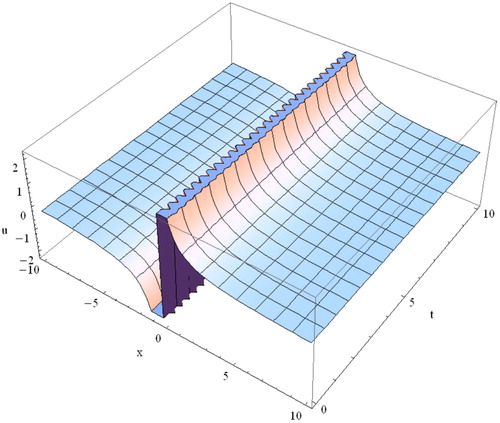Figure 3 indicates the nature of the periodic solution of $u_{1_5}\left(x,t\right).$ The figure of solution $u_{2_5}\left(x,t\right)$is eliminated here for minimalism. In the end, the solutions $u_{1_7}\left(x,t\right)$ and $u_{2_7}\left(x,t\right)$ represent the singular kink type. Figure 4 denotes the exact singular kink-type solution of $u_{1_7}\left(x,t\right).$ The figure of solution $u_{2_7}\left(x,t\right)$is analogous to the figure of solution $u_{1_7}\left(x,t\right),$ but for convenience it is omitted here.

Figure 1. Sketch of kink wave of $u_{1_2}(x,t)$ if $\lambda =-1,$ $d=1,$ $\sigma =1,$ $\alpha =\frac{1}{2},$$-10\le x\le 10,$ and 0$\le t\le 10.$

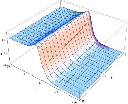
Figure 2. Sketch of multiple periodic wave of $u_{1_6}(x,t)$ if $\lambda =1,$ $d=1,$ $\sigma =0,$ $\alpha =\frac{1}{2},-10\le x\le 10,$ and 0$\le t\le 10.$

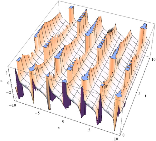
Figure 3. Shape of periodic wave of $u_{1_5}(x,t)$ if $\lambda =1,$ $d=-1,$ $\sigma =1,$ $\alpha =\frac{1}{2},$$-10\le x\le 10,$ and 0$\le t\le 10.$

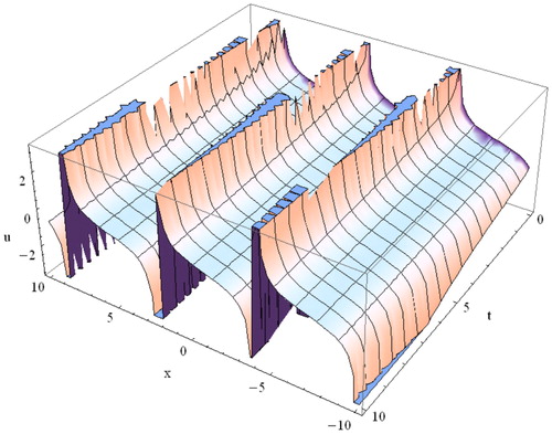
Figure 4. Shape of singular kink type wave of $u_{1_7}(x,t)$ if $\mu =1,$ $A_1=2,$ $A_2=1,$ $\alpha =\frac{1}{2},$$-10\le x\le 10,$ and 0$\le t\le 10.$

6. Comparison of the results

It is remarkable to observe that some of the obtained solutions demonstrate good similarity with earlier established solutions. A comparison of the solutions Roy et al. (2018), Batool and Ghazala (2018) and those obtained here are presented in Table 1 and Table 2.

Table 1. Comparison between Roy et al. (2018) solutions and our solutions to the STO equation

Roy et al. (2018)	Obtained solutions
If $c_0=0$ and $c_{00}\ne 0$ the solution becomes: $u_{1_1}\left(x,t\right)=\frac{\sqrt{\sigma }}{2p}\mathrm{ }\text{cot}\mathrm{h}\left\{\frac{\sqrt{\sigma }}{2p}\left(x+\frac{\omega t^{\alpha }}{\mathrm{\Gamma }\left(1+\alpha \right)}\right)\right\}.$	If $\sigma =0$ in Equation (4.8)(4.8) $$u_{1_3}\left(x,t\right)=\frac{\sqrt{-\lambda }}{2}\times \coth \left(\sqrt{-\lambda }(x+\frac{\frac{d\lambda }{4}{t}^{\alpha }}{\mathrm{\Gamma }\left(1+\alpha \right)})\right)\pm \frac{\sqrt{-\lambda \sigma }}{2}\times \mathit{cosech}\left(\sqrt{-\lambda }\right(x+\frac{\frac{d\lambda }{4}{t}^{\alpha }}{\mathrm{\Gamma }\left(1+\alpha \right)}\left)\right).$$(4.8) then our solution $u_{1_3}(x,t)$ becomes: $u_{1_3}\left(x,t\right)=\frac{\sqrt{-\lambda }}{2}\times \coth \left(\sqrt{-\lambda }(x+\frac{\frac{d\lambda }{4}{t}^{\alpha }}{\mathrm{\Gamma }\left(1+\alpha \right)})\right).$
If $c_0\ne 0$ and $c_{00}=0$ the solution becomes: $u_{2_1}\left(x,t\right)=\frac{\sqrt{\sigma }}{2p}\mathrm{ }\hspace{0.17em}\text{tan}\hspace{0.17em}\mathrm{h}\left\{\frac{\sqrt{\sigma }}{2p}\left(x+\frac{\omega t^{\alpha }}{\mathrm{\Gamma }\left(1+\alpha \right)}\right)\right\}.$	If $\sigma =0$ in Equation (4.7)(4.7) $$u_{1_2}\left(x,t\right)=\frac{\sqrt{-\lambda }}{2}\times \tanh \left(\sqrt{-\lambda }(x+\frac{\frac{d\lambda }{4}{t}^{\alpha }}{\mathrm{\Gamma }\left(1+\alpha \right)})\right)\pm \frac{\sqrt{-\lambda \sigma }}{2}\times \mathit{sech}\left(\sqrt{-\lambda }\right(x+\frac{\frac{d\lambda }{4}{t}^{\alpha }}{\mathrm{\Gamma }\left(1+\alpha \right)}\left)\right).$$(4.7) then our solution $u_{1_3}\left(x,t\right)$ becomes: $u_{1_2}\left(x,t\right)=\frac{\sqrt{-\lambda }}{2}\times \tanh \left(\sqrt{-\lambda }(x+\frac{\frac{d\lambda }{4}{t}^{\alpha }}{\mathrm{\Gamma }\left(1+\alpha \right)})\right).$
If $c_0=0$ and $c_{00}\ne 0$ then the solution becomes: $u_{3_1}\left(x,t\right)=\mathrm{i}\frac{\sqrt{\sigma }}{2p}\mathrm{ }\text{cot}\left\{\frac{\sqrt{-\sigma }}{2p}\left(x+\frac{\omega t^{\alpha }}{\mathrm{\Gamma }\left(1+\alpha \right)}\right)\right\}.$	If $\sigma =0$ in Equation (4.11)(4.11) $$u_{1_6}\left(x,t\right)=\frac{\sqrt{\lambda }}{2}\times \text{cot}\left(\sqrt{\lambda }(x+\frac{\frac{d\lambda }{4}{t}^{\alpha }}{\mathrm{\Gamma }\left(1+\alpha \right)})\right)\pm \frac{\sqrt{\lambda \sigma }}{2}\times \text{cosec}\left(\sqrt{\lambda }\right(x+\frac{\frac{d\lambda }{4}{t}^{\alpha }}{\mathrm{\Gamma }\left(1+\alpha \right)}\left)\right).$$(4.11) then our solution $u_{1_6}(x,t)$ becomes: $u_{1_6}\left(x,t\right)=\frac{\sqrt{\lambda }}{2}\times \text{cot}\left(\sqrt{\lambda }(x+\frac{\frac{d\lambda }{4}{t}^{\alpha }}{\mathrm{\Gamma }\left(1+\alpha \right)})\right).$
If $c_0\ne 0$ and $c_{00}=0$ then the solution becomes: $u_{3_1}\left(x,t\right)=-\mathrm{i}\frac{\sqrt{\sigma }}{2p}\mathrm{ }\text{cot}\left\{\frac{\sqrt{-\sigma }}{2p}\left(x+\frac{\omega t^{\alpha }}{\mathrm{\Gamma }\left(1+\alpha \right)}\right)\right\}.$	If $\sigma =0$ in Equation (4.10)(4.10) $$u_{1_5}\left(x,t\right)=\frac{\sqrt{\lambda }}{2}\times \text{tan}\left(\sqrt{\lambda }(x+\frac{\frac{d\lambda }{4}{t}^{\alpha }}{\mathrm{\Gamma }\left(1+\alpha \right)})\right)\pm \frac{\sqrt{\lambda \sigma }}{2}\times \text{sec}\left(\sqrt{\lambda }\right(x+\frac{\frac{d\lambda }{4}{t}^{\alpha }}{\mathrm{\Gamma }\left(1+\alpha \right)}\left)\right).$$(4.10) then our solution $u_{1_5}(x,t)$ becomes: $u_{1_5}\left(x,t\right)=\frac{\sqrt{\lambda }}{2}\times \text{tan}\left(\sqrt{\lambda }(x+\frac{\frac{d\lambda }{4}{t}^{\alpha }}{\mathrm{\Gamma }\left(1+\alpha \right)})\right).$

Table 2. Comparison between Batool and Ghazala (2018) solutions and our solutionsto the CA equation

Batool and Ghazala (2018)	Obtained solutions
If $A_1\ne 0$ and $A_2=0$ then the solution in Eq. (18) becomes: $u_8\left(\xi \right)$ = $\frac{1}{2}+\frac{1}{2}\tanh (\frac{x}{2\sqrt{2}}+\frac{3t^{\beta }}{4\mathrm{\Gamma }\left(1+\alpha \right)}).$	If $\sigma =0$ in Equation (4.18)(4.18) $$u_{2_2}\left(x,t\right)=\frac{1}{2}\pm \frac{1}{2}\times \tanh \left(\sqrt{-\lambda }\xi \right)\pm \mathrm{ }\times \frac{\sqrt{\lambda \sigma }}{2}s\mathit{ech}(\sqrt{-\lambda }\xi ),$$(4.18) then our solution $u_{2_2}(x,t)$ becomes: $u_{2_2}(x,t)$ = $\frac{1}{2}+\frac{1}{2}\times \tanh \left(\sqrt{-\lambda }\mathrm{ }(\sqrt{-\frac{1}{2\lambda }}x-\frac{3\mathrm{ }\sqrt{-\frac{1}{4\lambda }}{t}^{\alpha }}{\mathrm{\Gamma }(1+\alpha )})\right).$
If $A_1\ne 0$ and $A_2=0$ then the solution in Eq. (18) becomes: $u_{12}(\xi )$ = $\frac{1}{2}-\frac{1}{2}\tanh (\frac{x}{2\sqrt{2}}-\frac{3t^{\beta }}{4\mathrm{\Gamma }\left(1+\alpha \right)}).$	If $\sigma =0$ in Equation (4.18)(4.18) $$u_{2_2}\left(x,t\right)=\frac{1}{2}\pm \frac{1}{2}\times \tanh \left(\sqrt{-\lambda }\xi \right)\pm \mathrm{ }\times \frac{\sqrt{\lambda \sigma }}{2}s\mathit{ech}(\sqrt{-\lambda }\xi ),$$(4.18) then our solution $u_{2_2}(x,t)$ becomes: $u_{2_2}(x,t)$ = $\frac{1}{2}-\frac{1}{2}\times \tanh \left(\sqrt{-\lambda }\left(\sqrt{-\frac{1}{2\lambda }}x-\frac{3\mathrm{ }\sqrt{-\frac{1}{4\lambda }}{t}^{\alpha }}{\mathrm{\Gamma }\left(1+\alpha \right)}\right)\right).$

The hyperbolic and trigonometric function solutions referred to in Table 1 and the hyperbolic function solutions referred to in Table 2 are similar and if we set definite values of the arbitrary constants they are identical. It is important to understand that the travelling wave solution $u_{1_1}(x,t),$ $u_{1_4}(x,t),$ $u_{1_7}(x,t)u_{2_1}(x,t),$ $u_{2_3}\left(x,t\right),$ $u_{2_4}(x,t),$$u_{2_5}(x,t),$ $u_{2_6}(x,t)$ and $u_{2_7}(x,t)$ of the space time fractional Sharma–Tasso–Olver equation and the time fractional Cahn–Allen equation are all new and very important and were not originated in the previous work. These solutions are capable to solve the fission and fusion phenomena including for solitons, electromagnetic interactions, quantum relativistic atom theory, phase isolation in several components bass system, and the relativistic energy–momentum relation.

7. Conclusion

In this study, we investigate some fresh and more general solitary wave solutions of two NLFDEs, specifically, space time fractional STO and time fractional CA equation in terms of hyperbolic, trigonometric and rational function solution containing parameters. The obtained solutions to these equations is capable to put on the fission and fusion phenomena includes for solitons, quantum relativistic atom theory, phase isolation in several components bass system, the relativistic energy-momentum relation, electromagnetic interactions, etc. On the basis of our results obtained in this article, we might conclude that the competence of the double$(G\prime /G,1/G)$-expansion method is convenient, efficient and further general with respect to other methods and also be applicable to other NLFDEs.

Acknowledgements

The authors would like to express the deepest appreciation to the reviewers and editor for their valuable suggestions and comments to improve the article.

Disclosure Statement

We declare that none of the authors have any competing interests in this manuscript.

References

- Abdel-Salam, E. A. B., & Hassan, G. F. (2016). Multi-wave solutions of the space time fractional Burger and Sharma-Tasso-Olever equations. Ain Shams Engineering Journal, 7(1), 463–472. doi: 10.1016/j.asej.2015.04.001
- Akbar, M. A., & Ali, N. H. M. (2012). New solitary and periodic solutions of nonlinear evolution equation by exp- function method. World Applied Sciences Journal, 17(12), 1603–1610.
- Akbar, M. A., Ali, N. H. M., & Wazwaz, A. M. (2018). Closed form traveling wave solutions of non-linear fractional evolution equations through the modified simple equation method. Thermal Science, 22(1), 341–352. doi: 10.2298/TSCI170613097A
- Akbar, M. A., Ali, N. H. M., & Zayed, E. M. E. (2012a). A generalized and improved (G′/G)-expansion method for nonlinear evolution equation. Mathematical Problems in Engineering, 2012, 1–22. doi: 10.1155/2012/459879
- Akbar, M. A., Ali, N. H. M., & Zayed, E. M. E. (2012b). Abundant exact traveling wave solutions of the generalized Bretherton equation via the improved (G′/G)-expansion method. Communications in Theoretical Physics, 57(2), 173–178. doi: 10.1088/0253-6102/57/2/01
- Akgul, A., Baleanu, D., & Inc, M. (2016). On the solutions of electrohydrodynamic flow with fractional differential equations by reproducing kernel method. Open Physics, 14, 685–689.
- Alhakim, L. A., & Moussa, A. A. (2017). The improve exp(-ϕ(ξ))-expansion method and its application to non-linear fractional Sharma-Tasso-Olver equation. Journal of Applied & Computational Mathematics, 6(3), 1–5.
- Arafa, A. A. M., Rida, S. Z., & Mohamed, H. (2011). Homotopy analysis method for solving biological population model. Communications in Theoretical Physics, 56(5), 797–800. doi: 10.1088/0253-6102/56/5/01
- Ayhan, B., & Bekir, A. (2012). The (G′/G)-expansion method for the nonlinear lattice equations. Communications in Nonlinear Science and Numerical Simulation, 17(9), 3490–3498. doi: 10.1016/j.cnsns.2012.01.009
- Batool, F., & Ghazala, A. (2018). New solitary wave solutions of the time fractional Cahn-Allen equation via the improved (G′/G)-expansion method. The European Physical Journal Plus, 133(171), 1–11.
- Bekir, A., Aksoy, E., & Cevikel, A. C. (2016). Exact solutions of nonlinear time fractional differential equations by sub-equation method. Mathematical Methods in the Applied Science, 38(13), 2779–2784. doi: 10.1002/mma.3260
- Bekir, A., Guner, O., & Cevikel, A. C. (2013). Fractional complex transform and exp-function methods for fractional differential equations. Abstract and Applied Analysis, 2013, 426–462. doi: 10.1155/2013/426462
- Bekir, A., Guner, O., & Unsal, O. (2015). The first integral method for exact solutions of nonlinear fractional differential equation. Journal of Computational and Nonlinear Dynamics, 10(2), 021020.
- El-Sayed, A. M. A., Behiry, S. H., & Raslan, W. E. (2010). Adomian’s decomposition method for solving an intermediate fractional advection-dispersion equation. Computers and Mathematics with Applications, 59(5), 1759–1765. doi: 10.1016/j.camwa.2009.08.065
- Erturk, V. S., Momani, S., & Odibat, Z. (2008). Application of generalized transformation method to multi-order fractional differential equations. Communications in Nonlinear Science and Numerical Simulation, 13(8), 1642–1654.
- Esen, A., Yagmurlu, N. M., & Tasbozan, O. (2013). Approximate analytical solution to the time fractional damped Burger and Cahn-Allen equations. Applied Mathematics & Information Sciences, 7(5), 1951–1956. doi: 10.12785/amis/070533
- Gepreel, K. A. (2011). The homotopy perturbation method applied to the nonlinear fractional Kolmogorov-Petrovskii-Piskunov equations. Applied Mathematics Letters, 24(8), 1428–1434.
- Gepreel, K. A., & Omran, S. (2012). Exact solutions for nonlinear partial fractional differential equations. Chinese Physics B, 21(11), 110204. doi: 10.1088/1674-1056/21/11/110204
- Gómez-Aguilar, J. F., Martinez, H. Y., & Torres-Jimenez, J. (2017). Homotopy perturbation transform method for nonlinear differential equations involving to fractional operator with exponential kernel. Advances in Difference Equations, 2017(1), 68.
- Guo, S. M., & Mei, L. Q. (2011). The fractional variational iteration method using He’s polynomial. Physics Letters A, 375(3), 309–313. doi: 10.1016/j.physleta.2010.11.047
- Guo, S. M., Mei, L. Q., Li, Y., & Sun, Y. F. (2012). The improved fractional sub-equation method and its applications to the space-time fractional differential equations in fluid mechanics. Physics Letters A, 376(4), 407–411. doi: 10.1016/j.physleta.2011.10.056
- He, J. H. (2014). A tutorial review on fractal space-time and fractional calculus. International Journal of Theoretical Physics, 53(11), 3698–3718. doi: 10.1007/s10773-014-2123-8
- Islam, M. N., & Akbar, M. A. (2018). New exact wave solutions to the space-time fractional coupled Burgers equations and the space-time fractional foam drainage equation. Cogent Physics, 5, 1422957.
- Ji, J., Zhang, J. B., & Dong, Y. J. (2012). The fractional variational iteration method improved with the Adomian series. Applied Mathematics Letters, 25(12), 2223–2226. doi: 10.1016/j.aml.2012.06.007
- Jumarie, G. (2006). Modified Riemann-Liouville derivative and fractional Taylor series of non-differentiable functions further results. Computers & Mathematics with Applications, 51(9-10), 1367–1376. doi: 10.1016/j.camwa.2006.02.001
- Li, L. X., Li, E. Q., & Wang, M. L. (2010). The (G′/G,1/G)-expansion method and its application to travelling wave solutions of the Zakharov equations. Applied Mathematics A Journal of Chinese Universities, 25(4), 454–462.
- Liu, F. J., Liu, H. Y., Li, Z. B., & He, J. H. (2017). A delayed fractional model for cocoon heat-proof property. Thermal Science, 21(4), 1867–1871. doi: 10.2298/TSCI160415101L
- Lu, B. (2012). Backlund transformation of fractional Riccati equation and its applications to nonlinear fractional partial differential equations. Physics Letters A, 376(28-29), 2045–2048. doi: 10.1016/j.physleta.2012.05.013
- Martinez, H. Y., Gómez-Aguilar, J. F., & Atangana, A. (2018). First integral method for nonlinear differential equations with conformable derivative. Mathematical Modelling of Natural Phenomena, 13, 14–22. doi: 10.1051/mmnp/2018012
- Miller, K. S., & Ross, B. (1993). An introduction to the fractional calculus and fractional differential equations. New York: Wiley.
- Podlubny, I. (1999). Fractional differential equations. San Diego, CA: Academic.
- Rawashdeh, M. (2015). An efficient approach for time fractional damped Burger and time fractional Sharma-Tasso-Olever equations using the FRDTM. Applied Mathematics and Information Sciences, 9(3), 1239–1246.
- Rawashdeh, M. (2017). A reliable method for the space time fractional Burger and time fractional Cahn-Allen equations via the FRDTM. Advances in Difference Equations, 2017(1), 99. doi: 10.1186/s13662-0171148-8
- Roy, R., Akbar, M. A., & Wazwaz, A. M. (2018). Exact wave solutions for the non-linear time fractional Sharma-Tasso-Olver equation and the fractional Klein-Gordon equation by mathematical physics. Optical and Quantum Electronics, 50(1), 219–251.
- Seadawy, A. R. (2017a). The generalized nonlinear higher order of KdV equations from the higher order nonlinear Schrodinger equation and its solutions. Optik–International Journal for Light and Electron Optics, 139, 31–43. doi: 10.1016/j.ijleo.2017.03.086
- Seadawy, A. R. (2017b). Travelling wave solutions of a weakly nonlinear two-dimensional higher order Kadomtsev-Petviashvili dynamical equation for dispersive shallow water waves. The European Physical Journal Plus, 132(1), 29–38.
- Song, L. N., Wang, Q., & Zhang, H. (2009). Rational approximation solutions of the fractional Sharma-Tasso-Olever equation. Journal of Computational and Applied Mathematics, 224(1), 210–218. doi: 10.1016/j.cam.2008.04.033
- Uddin, M. H., Akbar, M. A., Khan, M. A., & Haque, M. A. (2017). Close form solutions of the fractional generalized reaction Duffing model and the density dependent fractional diffusion reaction equation. Applied and Computational Mathematics, 6(4), 177–184.
- Wang, M. L., Li, X. Z., & Zhang, J. L. (2008). The (G′/G)-expansion method and the traveling wave solutions of nonlinear evolution equations in mathematical physics. Physics Letters A, 372(4), 417–423. doi: 10.1016/j.physleta.2007.07.051
- Wang, K. L., & Wang, K. J. (2018). A modification of the reduced differential transform method for fractional calculus. Thermal Science, 22(4), 1871–1875. doi: 10.2298/TSCI1804871W
- Wang, Y., Zhang, Y.-F., & Liu, Z.-J. (2018). An application of local fractional variational iteration method and its application to local fractional modified Korteweg-de Vries equation. Thermal Science, 22(1 Part A), 23–27. doi: 10.2298/TSCI160501143W
- Wu, G. C. (2011). A fractional variational iteration method for solving fractional nonlinear differential equations. Computers and Mathematics with Applications, 61(8), 2186–2190. doi: 10.1016/j.camwa.2010.09.010
- Zayed, E. M. E., & Abdelaziz, M. A. M. (2012). The two variable (G′/G,1/G)-expansion method for solving the nonlinear KdV-mkdV equation. Mathematical Problems in Engineering, 2012, 1–14. doi: 10.1155/2012/725061
- Zhang, B. (2012). (G′/G)-expansion method for solving fractional partial differential equation in the theory of mathematical physics. Communications in Theoretical Physics, 58, 623–630.
- Zhang, S., & Zhang, H. Q. (2011). Fractional sub-equation method and its application to the nonlinear fractional PDEs. Physics Letters A, 375(7), 1069–1073. doi: 10.1016/j.physleta.2011.01.029