Application of the Exp (−φ(ζ))-expansion method for solitary wave solutions

Abstract

The solution of nonlinear mathematical models has much importance and in soliton theory its worth has increased. In present article, a research has been conducted of Caudrey-Dodd-Gibbon and Pochhammer-Chree (PC) equations, to discuss physics of these equations and to attain soliton solutions. $\text{Exp}\hspace{0.17em}$ $(-\phi (\zeta ))$-expansion technique is used to construct solitary wave solutions. Wave transformation is applied to convert problem in the form of ordinary differential equation. The drawn-out novel type outcomes play an essential role in the transportation of energy. It is noticed that under the study, the approach is extremely dependable and it may be prolonged to further mathematical models signified mostly in nonlinear differential equations.

Keywords:

• $\text{Exp}\hspace{0.17em}$ $(-\phi (\zeta ))$-expansion technique
• Caudrey-Dodd-Gibbon (CDG) equation
• Pochhammer-Chree (PC) equation
• Homogenous principal
• Solitary wave solution

1. Introduction

Recently solitary wave theory got some great improvements. Soliton wave occurrence enticed a number of researchers for its comprehensive applications in engineering and mathematical physics. First, J S Russell (by profession an engineer) contemplated on the solitary wave in 1834. In the form of differential equations, various physical occurrences in nature are modelled. The scientists made big efforts to get solution of such differential equations. To get soliton solutions, different attempts have been made by scientists. Modeling of various physical, biochemical and biological occurrences are in forms of nonlinear PDEs. The vigorous attainment is the headway for exact soliton solutions of mathematically modelled differential equations. Different mathematical techniques are developed. For the observation of physical activities of problem, exact solutions are vital. We have more applications and ability to examine the number of properties of mathematical model by utilizing the exact solution.

NLE equations play a very vital part in innumerable engineering and scientific arenas, such as, the heat flow, quantum mechanics, solid state physics, chemical kinematics, fluid mechanics, optical fibres, plasma physics, the wave proliferation phenomena, proliferation of shallow water waves, etc.

Therefore, different techniques for finding exact solutions are used for a diversified field of partial differential equations like, homogenious balance technique for example (Wang, 1995; Zayed et al., 2004), Hirota’s bilinear approach (Hirota, 1973; Hirota & Satsuma, 1981), Auxiliary equivalence technique (Sirendaoreji, 2004), Trial task technique (Inc & Evans, 2004), Jacobi elliptic task system (Ali, 2011), Tanh-function technique (Abdou, 2007), and method of sine-cosine (Wazwaz, 2004), truncated Painleve expansion technique (Weiss et al., 1983), variational iteration method (VIM) (Abbasbandy, 2007), Exp-function technique (He & Wu, 2006; Akbar & Ali, 2012), $(G\mathrm{\prime }/G)$-expansion approach (Wang et al., 2008; Akbar et al., 2012; Zayed, 2010; Zayed & Gepreel, 2009; Shehata, 2010; Zhang et al., 2010), Exact soliton solution (Khan & Akbar, 2013; Liping et al., 2009; Zhang et al., 2013). Several theoretical and experimental works for solitons includes (Wang et al., 2017; Dai et al., 2018; Wang et al., 2016; Wang et al., 2018; Ding et al., 2017). On exact solution, some novel results and computational methods involved to travelling-wave transformation, see the references (Yang, 2016; Yang et al., 2016, 2017; Saad et al., 2017; Yang & Feng, 2017; Feng et al., 2017). Some recent studies on exact soliton solutions are (Hu & Li, 2018; Islam et al., 2017; Kaplan & Akbulut, 2018; Zayed & Al-Nowehy, 2017).

In this paper, our basic motive is to discuss physics of nonlinear CDG and PC equation, and also to obtain soliton like solutions of these equation through a much authentic and productive method that is notable in literature as $\text{exp}\hspace{0.17em}$ $(-\phi (\zeta ))$-expansion technique. The analytical results are very stimulated. From the technique, the solution procedure is quite simple, clear and all types of NLEEs are easily expanded. This technique simply emphasises to obtain the solution of PDE that is indicated in the kind of polynomial in $\text{exp}\hspace{0.17em}$ $(-\phi (\zeta )),$ and $(-\phi (\zeta ))$ must satisfies the ODE. (1.1) $${\phi }^{\prime }\left(\zeta \right)=\hspace{0.17em}\text{exp}\hspace{0.17em}\left(-\phi \left(\zeta \right)\right)+\mu \hspace{0.17em}\text{exp}\hspace{0.17em}\left(\phi \left(\zeta \right)\right)+\lambda .$$(1.1)

We know $$\zeta =x+y+z-\omega t.$$

By homogenous principle, the degree of polynomial is obtained. We accomplish a set of algebraic equation by balancing the highest order derivative with nonlinear terms. The article is divided in to various segments. In the next segment, we study analysis of method to obtain the soliton waves solution. The third segment is appropriate to discuss physics of nonlinear equations and for application of $\text{exp}\hspace{0.17em}$ $(-\phi (\zeta ))$-expansion method. In the last section, we drew some conclusions by discussing the results.

2. Analysis of method

In general, nonlinear partial differential equation (NPDE) can be written as: (2.1) $$F\left(\eta ,{\eta }_x,{\eta }_y,{\eta }_z,{\eta }_{\mathit{xx}},{\eta }_{\mathit{xy}},{\eta }_{\mathit{xz}},\dots \right)=0.$$(2.1)

Where $\eta \left(x,y,z,t\right)$ is to be unknown, $F$ is the polynomial in $\eta (x,y,z,t)$ and different derivatives of $\eta (x,y,z,t)$ involving nonlinear terms and highest order differential. Using $\text{Exp}\hspace{0.17em}$ $(-\phi (\zeta ))$-expansion method, we follow steps given below in detail,

Step1: Invoking a wave transformation: (2.2) $$\zeta =x+y+z-\omega t.$$(2.2)

Here $\omega$ represent wave speed. Applying wave transformation into equation (2.1)(2.1) $$F\left(\eta ,{\eta }_x,{\eta }_y,{\eta }_z,{\eta }_{\mathit{xx}},{\eta }_{\mathit{xy}},{\eta }_{\mathit{xz}},\dots \right)=0.$$(2.1) we got an ODE: (2.3) $$G(\eta ,\eta {}^{\prime },\eta {}^{″},\eta {}^{″\prime },\dots )=0.$$(2.3)

In (2.3)(2.3) $$G(\eta ,\eta {}^{\prime },\eta {}^{″},\eta {}^{″\prime },\dots )=0.$$(2.3) , derivative w.r.t $\zeta$ are symbolized by prime. If it is needed, integrate equation (2.3)(2.3) $$G(\eta ,\eta {}^{\prime },\eta {}^{″},\eta {}^{″\prime },\dots )=0.$$(2.3) and set constant of integration equal to zero.

Step 2: Solution of equation (2.3)(2.3) $$G(\eta ,\eta {}^{\prime },\eta {}^{″},\eta {}^{″\prime },\dots )=0.$$(2.3) is expressed in the form of a polynomial in $\text{exp}\hspace{0.17em}$ $(-\phi (\zeta ))$ as: (2.4) $$\eta \left(\zeta \right)=a_n{(\hspace{0.17em}\text{exp}\hspace{0.17em}(-\phi \left(\zeta \right)\left)\right)}^n+a_{n-1}{(\hspace{0.17em}\text{exp}\hspace{0.17em}(-\phi \left(\zeta \right)\left)\right)}^{n-1}+\cdots ,$$(2.4)

In the equation (2.4)(2.4) $$\eta \left(\zeta \right)=a_n{(\hspace{0.17em}\text{exp}\hspace{0.17em}(-\phi \left(\zeta \right)\left)\right)}^n+a_{n-1}{(\hspace{0.17em}\text{exp}\hspace{0.17em}(-\phi \left(\zeta \right)\left)\right)}^{n-1}+\cdots ,$$(2.4) $a_n,a_{n-1},\dots$ are the arbitrary constants which are to be evaluated such that $a_n\ne 0.$ Also $\phi (\zeta )$ satisfies equation (1.1)(1.1) $${\phi }^{\prime }\left(\zeta \right)=\hspace{0.17em}\text{exp}\hspace{0.17em}\left(-\phi \left(\zeta \right)\right)+\mu \hspace{0.17em}\text{exp}\hspace{0.17em}\left(\phi \left(\zeta \right)\right)+\lambda .$$(1.1) .

Step 3: In this step, we calculate value of $n$ by using homogeneous balance principle.

Case 1:

For ${\lambda }^2-4\mu >0$ and $\mu \ne 0,$ (2.5) $$\phi \left(\zeta \right)=\hspace{0.17em}\text{ln}\hspace{0.17em}\left\{\frac{1}{2\mu }\right(-\sqrt{{\lambda }^2-4\mu }\tanh \left(\frac{\sqrt{{\lambda }^2-4\mu }}{2}\right(\zeta +c_1\left)\right)-\lambda \left)\right\}.$$(2.5)

Where $c_1$ is constant of integration. $$

Case 2:

For ${\lambda }^2-4\mu <0$ and $\mu \ne 0,$ (2.6) $$\phi \left(\zeta \right)=\hspace{0.17em}\text{ln}\hspace{0.17em}\left\{\frac{1}{2\mu }\right(-\lambda +\sqrt{4\mu -{\lambda }^2}\left(\frac{\sqrt{4\mu -{\lambda }^2}}{2}\right(\zeta +c_1\left)\right)\left)\right\}.$$(2.6)

Case 3:

For $\lambda \ne 0$ and $\mu =0,$ (2.7) $$\phi \left(\zeta \right)=-\hspace{0.17em}\text{ln}\hspace{0.17em}\left\{\frac{\lambda }{(\hspace{0.17em}\text{exp}\hspace{0.17em}(\lambda (\zeta +c_1))-1)}\right\}.$$(2.7)

Case 4:

For ${\lambda }^2-4\mu =0$ and $\mu \ne 0,$ $\lambda \ne 0,$ (2.8) $$\phi \left(\zeta \right)=\hspace{0.17em}\text{ln}\hspace{0.17em}\left\{\frac{2\left(\lambda \right(\zeta +c_1\left)\right)+2}{{\lambda }^2(\zeta +c_1)}\right\}.$$(2.8)

Case 5:

For $\lambda =0$ and $\mu =0,$ (2.9) $$\phi \left(\zeta \right)=\hspace{0.17em}\text{ln}\hspace{0.17em}\left(\zeta +c_1\right).$$(2.9)

Step 4: In this step, we insert polynomial given in (2.4)(2.4) $$\eta \left(\zeta \right)=a_n{(\hspace{0.17em}\text{exp}\hspace{0.17em}(-\phi \left(\zeta \right)\left)\right)}^n+a_{n-1}{(\hspace{0.17em}\text{exp}\hspace{0.17em}(-\phi \left(\zeta \right)\left)\right)}^{n-1}+\cdots ,$$(2.4) into ODE (2.3)(2.3) $$G(\eta ,\eta {}^{\prime },\eta {}^{″},\eta {}^{″\prime },\dots )=0.$$(2.3) and then use equation (1.1)(1.1) $${\phi }^{\prime }\left(\zeta \right)=\hspace{0.17em}\text{exp}\hspace{0.17em}\left(-\phi \left(\zeta \right)\right)+\mu \hspace{0.17em}\text{exp}\hspace{0.17em}\left(\phi \left(\zeta \right)\right)+\lambda .$$(1.1) . The left-hand side of nonlinear ODE is converted in the form of a polynomial in Exp-$(-\phi (\zeta )).$ We put each coefficient of polynomial equal to zero, results in attain a set of algebraic equations for $a_n,\dots ,\omega ,\lambda$ and $\mu .$

Step 5: In this step, with the help of symbolic computation software like Maple 18, the values of the constants $a_n,\dots ,\mathrm{ }\omega ,\lambda ,\mu$ are computed. Replacing values of these constants into equation (2.4)(2.4) $$\eta \left(\zeta \right)=a_n{(\hspace{0.17em}\text{exp}\hspace{0.17em}(-\phi \left(\zeta \right)\left)\right)}^n+a_{n-1}{(\hspace{0.17em}\text{exp}\hspace{0.17em}(-\phi \left(\zeta \right)\left)\right)}^{n-1}+\cdots ,$$(2.4) , we obtain soliton wave solutions.

3. Applications of method

This section is divided into two sub sections. Both Caudrey-Dodd-Gibbon (CDG) and Pochhammer-Chree (PC) equations are studied physically, then $\text{exp}$ $(-\phi (\zeta ))$-expansion technique is applied to attain solitary wave solutions of these nonlinear differential equations. The attained results are quite efficient and motivating.

3.1. Solution of Caudrey-Dodd-Gibbon Equation

The general form of the fifth order KdV equation is written as: (3.1) $${\eta }_t+\alpha {\eta }_{\mathit{xxxxx}}+\sigma \eta {\eta }_{\mathit{xxx}}+\gamma {\eta }_x{\eta }_{\mathit{xx}}+\delta {\eta }^2{\eta }_x=0.$$(3.1)

In above equation $\alpha ,\sigma ,\gamma$ and $\delta$ are arbitrary real parameters. By setting $\alpha =1,\sigma =\beta ,\gamma =\beta$ and $\delta =\frac{1}{5}{\beta }^2$ we obtain, (3.2) $${\eta }_t+\frac{1}{5}{\beta }^2{\eta }^2{\eta }_x+\beta {\eta }_x{\eta }_{\mathit{xx}}+\beta \eta {\eta }_{\mathit{xxx}}+{\eta }_{\mathit{xxxxx}}=0.$$(3.2)

Which is known as CDG equation. This equation describes the evolution of quasi one-dimensional shallow water waves when it affects the surface tension; and the viscosity are negligible. Shallow water waves are produced when depth of water is less than one half of the wavelength of wave. Their speed is independent of their wavelength too. It depends, however, on the depth of the water. Shallow water waves show no dispersion.

Introducing a transformation as $$\zeta =x+y+z-\omega t.$$ (3.3) $$-\omega {\eta }^{\prime }+\frac{1}{5}{\beta }^2{\eta }^2{\eta }^{\prime }+\beta {\eta }^{\prime }{\eta }^{″}+\beta \eta {\eta }^{‴}+{\eta }^{\left(v\right)}=0.$$(3.3)

On integrating we have, (3.4) $$A-\omega \eta +\frac{1}{15}{\beta }^2{\eta }^3+\beta \eta {\eta }^{″}+{\eta }^{\left(\mathit{iv}\right)}=0.$$(3.4)

Here $A$ is the constant of integration and prime symbolizes the derivative w.r.t. $\zeta .$ Now for value of $n,$ we balance the highest order linear term with the highest order non-linear term of equation (3.4)(3.4) $$A-\omega \eta +\frac{1}{15}{\beta }^2{\eta }^3+\beta \eta {\eta }^{″}+{\eta }^{\left(\mathit{iv}\right)}=0.$$(3.4) . We attain $n=2.$ So equation (2.4)(2.4) $$\eta \left(\zeta \right)=a_n{(\hspace{0.17em}\text{exp}\hspace{0.17em}(-\phi \left(\zeta \right)\left)\right)}^n+a_{n-1}{(\hspace{0.17em}\text{exp}\hspace{0.17em}(-\phi \left(\zeta \right)\left)\right)}^{n-1}+\cdots ,$$(2.4) reduces to: (3.5) $$\eta \left(\zeta \right)=a_0+a_1{e}^{-\phi \left(\zeta \right)}+{\left(e^{-\phi \left(\zeta \right)}\right)}^2.$$(3.5)

Here $a_0\mathrm{ }\mathit{and}\mathrm{ }{a}_1,\mathrm{ }{a}_2$ are the constants which are to be calculated.

By making use of (3.5)(3.5) $$\eta \left(\zeta \right)=a_0+a_1{e}^{-\phi \left(\zeta \right)}+{\left(e^{-\phi \left(\zeta \right)}\right)}^2.$$(3.5) into (3.4)(3.4) $$A-\omega \eta +\frac{1}{15}{\beta }^2{\eta }^3+\beta \eta {\eta }^{″}+{\eta }^{\left(\mathit{iv}\right)}=0.$$(3.4) , we transformed the left-hand side into a polynomial in $e^{-\phi (\zeta )}.$ We put each coefficient of this polynomial equal to zero and attain a set of algebraic equations for $a_0,a_1,a_2,\lambda ,\mu ,A$ and $\omega$ as follow: $$-\omega a_1+\frac{1}{5}{\mathrm{\beta }}^2{a}^2{a}_1+22a_1\mu {\lambda }^2+120a_2{\mu }^2\lambda +30a_2{\lambda }^3\mu +6\mathrm{\beta }{a}_0{a}_2\mu \lambda +\mathrm{\beta }{a}_0{a}_1{\lambda }^2+2\mathrm{\beta }a{a}_1\mu +2\mathrm{\beta }{a}_1{a}_2{\mu }^2+\mathrm{\beta }{a}_1^2\mu \lambda +16a_1{\mu }^2+a_1{\lambda }^4=0.$$ $$\frac{1}{5}{\mathrm{\beta }}^2{a_0}^2{a}_2+\frac{1}{5}{\mathrm{\beta }}^2{a_1}^2{a}_0+2\mathrm{\beta }{a_1}^2\mu +60a_1\mu \lambda +232a_2{\lambda }^2\mu +2\mathrm{\beta }{a}_2^2{\mu }^2+\mathrm{\beta }{a}_1^2{\lambda }^2+7\mathrm{\beta }{a}_1{a}_2\mu \lambda +8\mathrm{\beta }{a}_0{a}_2\mu +3\mathrm{\beta }{a}_0{a}_1\lambda +4\mathrm{\beta }{a}_0{a}_2{\lambda }^2+136a_2{\mu }^2+16a_2{\lambda }^4-\omega a_2+15a_1{\lambda }^3=0.$$ $$440a_2\mu \lambda +2\mathrm{\beta }{a}_0{a}_1+3\mathrm{\beta }{a}_1^2\lambda +\frac{2}{5}{\mathrm{\beta }}^2{a}_0{a}_1{a}_2+10\mathrm{\beta }{a}_1{a}_2\mu +6\mathrm{\beta }{a}_2^2\mu \lambda +10\mathrm{\beta }{a}_0{a}_2\lambda +5\mathrm{\beta }{a}_1{a}_2{\lambda }^2+\frac{1}{15}{\mathrm{\beta }}^2{a}_1^3+40a_1\mu +130a_2{\lambda }^3+50a_1{\lambda }^2=0.$$ $$\frac{1}{5}{\mathrm{\beta }}^2{a}_0{a}_2^2+\frac{1}{5}{\mathrm{\beta }}^2{a}_1^2{a}_2+8\mathrm{\beta }{a}_2^2\mu +6\mathrm{\beta }{a}_0{a}_2+4\mathrm{\beta }{a}_2^2{\lambda }^2+13\mathrm{\beta }{a}_1{a}_2\lambda +240a_2\mu +330a_2{\lambda }^2+2\mathrm{\beta }{a}_1^2+60a_1\lambda =0.$$ $$\frac{1}{5}{\mathrm{\beta }}^2{a}_1{a}_2^2+8\mathrm{\beta }{a}_1{a}_2+10\mathrm{\beta }{a}_2^2\lambda +336a_2\lambda +24a_1=0.$$ $$6\mathrm{\beta }{a}_2^2+\frac{1}{15}{\mathrm{\beta }}^2{a}_2^3+120a_2=0.$$ $$A-\omega a_0+\frac{1}{15}{\mathrm{\beta }}^2{a}_0^3+a_1\mu {\lambda }^3+8a_1{\mu }^2\lambda +14a_2{\mu }^2{\lambda }^2+16a_2{\mu }^3+\mathrm{\beta }{a}_0{a}_1\mu \lambda +2\mathrm{\beta }{a}_0{a}_2{\mu }^2=0.$$

With the help of symbolic computation software like Maple 18 algebraic equations are solved. Finally, we obtain the following solution set:

1^st Solution Set:

Consider the solution set of the form $$\omega =\frac{1}{5}{\mathrm{\beta }}^2{a}_0^2+\mathrm{\beta }{a}_0{\lambda }^2+22\mu {\lambda }^2+76{\mu }^2+{\lambda }^4+8\mathrm{\beta }{a}_0\mu ,$$ $$a_0=a_0,\mathrm{ }{a}_1=-\frac{30\lambda }{\mathrm{\beta }},\mathrm{ }{a}_2=-\frac{30}{\mathrm{\beta }},$$ $$A=\frac{1}{15\mathrm{\beta }}\left(\begin{array}{c}2{\mathrm{\beta }}^3{a}_0^3+15{\mathrm{\beta }}^2{a}_0^2{\lambda }^2+780a_0{\lambda }^2\mu \beta \\ +2040a_0{\mu }^2\beta +15\beta a_0{\lambda }^4+120{\mathrm{\beta }}^2{a}_0^2\mu \\ +450\mu {\lambda }^4+9900{\mu }^2{\lambda }^2+7200{\mu }^3\end{array}\right).$$

By using above values into equation (3.5)(3.1) $${\eta }_t+\alpha {\eta }_{\mathit{xxxxx}}+\sigma \eta {\eta }_{\mathit{xxx}}+\gamma {\eta }_x{\eta }_{\mathit{xx}}+\delta {\eta }^2{\eta }_x=0.$$(3.1) , we obtain: (3.6) $$\eta =-\frac{-\beta a_0+30e^{-\phi \left(\zeta \right)}\lambda +30e^{-2\phi \left(\zeta \right)}}{\beta }.$$(3.6)

Where $$\zeta =x+y+z-\omega t.$$

Inserting the solutions of (1.1)(1.1) $${\phi }^{\prime }\left(\zeta \right)=\hspace{0.17em}\text{exp}\hspace{0.17em}\left(-\phi \left(\zeta \right)\right)+\mu \hspace{0.17em}\text{exp}\hspace{0.17em}\left(\phi \left(\zeta \right)\right)+\lambda .$$(1.1) in (3.6)(3.6) $$\eta =-\frac{-\beta a_0+30e^{-\phi \left(\zeta \right)}\lambda +30e^{-2\phi \left(\zeta \right)}}{\beta }.$$(3.6) , we attain five cases of soliton wave solutions for CDG equation.

Case 1:

When ${\lambda }^2-4\mu >0$ and $\mu \ne 0,$ we attain solution, (3.7) $${\eta }_{11}=\frac{1}{\mathrm{\beta }}\left({\mathrm{\beta }a}_0-\frac{\left(60\mu \lambda \right)}{-\sqrt{{\lambda }^2-4\mu }\tanh \left(\frac{1}{2}\sqrt{{\lambda }^2-4\mu }\left(\zeta +c_1\right)\right)-\lambda \mathrm{ }}-\frac{\left(120{\mu }^2\right)}{{\left(-\sqrt{{\lambda }^2-4\mu }\tanh \left(\frac{1}{2}\sqrt{{\lambda }^2-4\mu }\left(\zeta +c_1\right)\right)-\lambda \right)}^2\mathrm{ }}\right).$$(3.7)

Case 2:

When ${\lambda }^2-4\mu <0$ and $\mu \ne 0,$ then we have, (3.8) $${\eta }_{12}=\frac{1}{\mathrm{\beta }}\left({\mathrm{\beta }a}_0-\frac{\left(60\mu \lambda \right)}{\sqrt{-{\lambda }^2+4\mu }\text{tan}\left(\frac{1}{2}\sqrt{-{\lambda }^2+4\mu }\left(\zeta +c_1\right)\right)-\lambda \mathrm{ }}-\frac{\left(120{\mu }^2\right)}{{\left(\sqrt{{-\lambda }^2+4\mu }\tanh \left(\frac{1}{2}\sqrt{{-\lambda }^2+4\mu }\left(\zeta +c_1\right)\right)-\lambda \right)}^2\mathrm{ }}\right).$$(3.8)

Case 3:

When $\mu =0$ and $\lambda \ne 0,$ we attain, (3.9) $${\eta }_{13}=\frac{1}{\mathrm{\beta }}\left({\mathrm{\beta }a}_0-\frac{30{\lambda }^2}{\exp \left(\lambda \left(\zeta +c_1\right)\right)-1}-\frac{30{\lambda }^2}{{\left(\exp \left(\lambda \left(\zeta +c_1\right)\right)-1\right)}^2}\right).$$(3.9)

Case 4:

When ${\lambda }^2-4\mu =0,\mathrm{ }\mu =0$ and $\lambda \ne 0,$ (3.10) $${\eta }_{14}=-\frac{1}{\mathrm{\beta }}\left({-\mathrm{\beta }a}_0+\frac{30{\lambda }^3\left(\zeta +c_1\right)}{-4+\left(-2\zeta -2c_1\right)\lambda }+\frac{30{\lambda }^4{\left(\zeta +c_1\right)}^2}{{\left(-4+\left(-2\zeta -2c_1\right)\lambda \right)}^2}\right).$$(3.10)

Case 5:

When $\mu =0$ and $\lambda =0,$ we attain the solution as, (3.11) $${\eta }_{15}=\frac{1}{\mathrm{\beta }}\left({\mathrm{\beta }a}_0-30e^{-2ln\left(\zeta +c_1\right)}\right).$$(3.11)

Where $$\zeta =x-(\frac{1}{5}{\mathrm{\beta }}^2{a}_0^2+\mathrm{\beta }{a}_0{\lambda }^2+22\mu {\lambda }^2+76{\mu }^2+{\lambda }^4+8\mathrm{\beta }{a}_0\mu )t.$$

2^nd Solution Set:

Consider the solution set of the form: $$\omega ={\lambda }^4-8\mu {\lambda }^2+16{\mu }^2,\mathrm{ }{a}_0=-\frac{5\left({\lambda }^2+8\mu \right)}{\mathrm{\beta }},\mathrm{ }{a}_1=-\frac{60\lambda }{\mathrm{\beta }},$$ (3.12) $$a_2=-\frac{60}{\mathrm{\beta }},\mathrm{ }A=-\frac{10}{3\mathrm{\beta }}\left(-{\lambda }^6-48{\mu }^2{\lambda }^2+64{\mu }^3+12\mu {\lambda }^4\mu \right).$$(3.12)

Using values given in equation (3.12)(3.12) $$a_2=-\frac{60}{\mathrm{\beta }},\mathrm{ }A=-\frac{10}{3\mathrm{\beta }}\left(-{\lambda }^6-48{\mu }^2{\lambda }^2+64{\mu }^3+12\mu {\lambda }^4\mu \right).$$(3.12) into equation (3.5)(3.5) $$\eta \left(\zeta \right)=a_0+a_1{e}^{-\phi \left(\zeta \right)}+{\left(e^{-\phi \left(\zeta \right)}\right)}^2.$$(3.5) , we obtain (3.13) $$\eta =-\frac{5\left({\mathrm{\lambda }}^2+8\mathrm{\mu }+12e^{-\phi \left(\zeta \right)}\mathrm{ }\mathrm{\lambda }+12e^{-2\phi \left(\zeta \right)}\right)}{\mathrm{\beta }}.$$(3.13)

Where $$\zeta =x+y+z-\omega t.$$

Replacing the solutions of equation (1.1)(1.1) $${\phi }^{\prime }\left(\zeta \right)=\hspace{0.17em}\text{exp}\hspace{0.17em}\left(-\phi \left(\zeta \right)\right)+\mu \hspace{0.17em}\text{exp}\hspace{0.17em}\left(\phi \left(\zeta \right)\right)+\lambda .$$(1.1) into equation (3.13)(3.13) $$\eta =-\frac{5\left({\mathrm{\lambda }}^2+8\mathrm{\mu }+12e^{-\phi \left(\zeta \right)}\mathrm{ }\mathrm{\lambda }+12e^{-2\phi \left(\zeta \right)}\right)}{\mathrm{\beta }}.$$(3.13) , we get five cases of soliton wave solutions for the Caudrey-Dodd-Gibbon (CDG) equation:

Case 1:

When ${\lambda }^2-4\mu >0$ and $\mu \ne 0,$ we attain solution, (3.14) $${\eta }_{21}=\mathrm{ }\frac{1}{\mathrm{\beta }}\left(-5{\mathrm{\lambda }}^2-40\mathrm{\mu }-\frac{\left(120\mu \lambda \right)}{-\sqrt{{\lambda }^2-4\mu }\tanh \left(\frac{1}{2}\sqrt{{\lambda }^2-4\mu }\left(\zeta +c_1\right)\right)-\lambda \mathrm{ }}-\mathrm{ }\frac{\left(240{\mu }^2\right)}{{\left(-\sqrt{{\lambda }^2-4\mu }\tanh \left(\frac{1}{2}\sqrt{{\lambda }^2-4\mu }\left(\zeta +c_1\right)\right)-\lambda \right)}^2\mathrm{ }}\right).$$(3.14)

Case 2:

When ${\lambda }^2-4\mu <0$ and $\mu \ne 0,$ we attain the solution, (3.15) $${\eta }_{22}=\frac{1}{\mathrm{\beta }}\left(-5{\mathrm{\lambda }}^2-40\mathrm{\mu }-\frac{\left(120\mu \lambda \right)}{\sqrt{-{\lambda }^2+4\mu }\text{tan}\left(\frac{1}{2}\sqrt{{-\lambda }^2+4\mu }\left(\zeta +c_1\right)\right)-\lambda \mathrm{ }}-\mathrm{ }\frac{\left(240{\mu }^2\right)}{{\left(\sqrt{{-\lambda }^2+4\mu }\tanh \left(\frac{1}{2}\sqrt{{-\lambda }^2+4\mu }\left(\zeta +c_1\right)\right)-\lambda \right)}^2\mathrm{ }}\right).$$(3.15)

Case 3:

When $\mu =0$ and $\lambda \ne 0,$ we obtain the solution, (3.16) $${\eta }_{23}=\frac{1}{\mathrm{\beta }}\left(-5{\mathrm{\lambda }}^2-\frac{60{\lambda }^2}{\exp \left(\lambda \left(\zeta +c_1\right)\right)-1}-\frac{60{\lambda }^2}{{\left(\exp \left(\lambda \left(\zeta +c_1\right)\right)-1\right)}^2}\right).$$(3.16)

Case 4:

When ${\lambda }^2-4\mu =0,\mathrm{ }\mu =0$ and $\lambda \ne 0,$ we have the solution, (3.17) $${\eta }_{24}=-\frac{1}{\mathrm{\beta }}\left(5\left({\mathrm{\lambda }}^2+8\mathrm{\mu }+\frac{12{\lambda }^3\left(\zeta +c_1\right)}{-4+\left(-2\zeta -2c_1\right)\lambda }+\frac{12{\lambda }^4{\left(\zeta +c_1\right)}^2}{{\left(-4+\left(-2\zeta -2c_1\right)\lambda \right)}^2}\right)\right).$$(3.17)

Case 5:

When $\mu =0$ and $\lambda =0,$ we attain the solution, (3.18) $${\eta }_{25}=-\frac{60}{\mathrm{\beta }{\left(\zeta +c_1\right)}^2}\mathrm{ }.$$(3.18)

Here $$\varsigma =x-({\lambda }^4-8\mu {\lambda }^2+16{\mu }^2)t$$

3.2. Solution of Pochhammer-Chree Equation

The generalized Pochhammer-Chree (PC) equation is given by, $${\eta }_{\mathit{tt}}-{\eta }_{\mathit{ttxx}}-{\left(\mathrm{a}\eta -\mathrm{b}{\eta }^{\mathrm{n}+1}-\mathrm{\gamma }{\eta }^{2\mathrm{n}+1}\right)}_{\mathrm{xx}}=0.$$

Taking n = 2, we have, $${\eta }_{\mathit{tt}}-{\eta }_{\mathit{ttxx}}-{\left(\mathrm{a}\eta -\mathrm{b}{\eta }^3-\mathrm{\gamma }{\eta }^5\right)}_{\mathrm{xx}}=0.$$

Where $a,b$ and $\gamma$ are arbitrary non-zero constants, while the exponent $n\left(>1\right)$ is the power law nonlinearity parameter. This equation represents a nonlinear model of longitudinal wave propagation of elastic rods. Longitudinal waves are waves in which the displacement of the medium is in the same direction as, or the opposite direction to, the direction of propagation of the wave. Longitudinal waves include sound waves and particle velocity propagated in an elastic medium.

Let us consider $\mathrm{ }\gamma =0,$ the above equation becomes, (3.19) $${\eta }_{\mathit{tt}}-{\eta }_{\mathit{ttxx}}-{\left(\mathrm{a}\eta -\mathrm{b}{\eta }^3\right)}_{\mathrm{xx}}=0.$$(3.19)

Introducing a transformation as $\xi =x+y+z-\omega t$ equation (3.19)(3.19) $${\eta }_{\mathit{tt}}-{\eta }_{\mathit{ttxx}}-{\left(\mathrm{a}\eta -\mathrm{b}{\eta }^3\right)}_{\mathrm{xx}}=0.$$(3.19) can be converted to an ordinary differential equation. $${\omega }^2{\eta }^{\text{″}}-{\omega }^2{\eta }^{\text{″″}}-\mathrm{a}{\eta }^{\text{″}}+6b\eta {\left({\eta }^{\mathrm{\prime }}\right)}^2+3b{\eta }^2{\eta }^{\text{″}}=0.$$

Integrating twice, we have, (3.20) $$A+B\xi +{\omega }^2\eta -\mathrm{a}\eta +\mathrm{b}{\eta }^3-{\omega }^2{\eta }^{\text{″}}=0.$$(3.20)

Here $A$ and $B$ are the constants of integration and prime symbolizes the derivative w.r.t. $\zeta .$ Now for value of $n,$ we balance the highest order linear term with the highest order non-linear term of equation (3.20)(3.20) $$A+B\xi +{\omega }^2\eta -\mathrm{a}\eta +\mathrm{b}{\eta }^3-{\omega }^2{\eta }^{\text{″}}=0.$$(3.20) . We attain $n=1.$ So equation (2.4)(2.4) $$\eta \left(\zeta \right)=a_n{(\hspace{0.17em}\text{exp}\hspace{0.17em}(-\phi \left(\zeta \right)\left)\right)}^n+a_{n-1}{(\hspace{0.17em}\text{exp}\hspace{0.17em}(-\phi \left(\zeta \right)\left)\right)}^{n-1}+\cdots ,$$(2.4) reduces to, (3.21) $$\eta \left(\zeta \right)=a_0+a_1{e}^{-\phi \left(\zeta \right)}.$$(3.21)

Here $a_0\mathrm{ }\mathit{and}\mathrm{ }{a}_1$ are the constants which are to be calculated.

By making use of (3.21)(3.21) $$\eta \left(\zeta \right)=a_0+a_1{e}^{-\phi \left(\zeta \right)}.$$(3.21) into (3.20)(3.20) $$A+B\xi +{\omega }^2\eta -\mathrm{a}\eta +\mathrm{b}{\eta }^3-{\omega }^2{\eta }^{\text{″}}=0.$$(3.20) , we transformed the left-hand side into a polynomial in $e^{-\phi (\zeta )}.$ We put each coefficient of this polynomial equal to zero, and attain a set of algebraic equations for $a_0,a_1,a_2,\lambda ,\mu ,A,B$ and $\omega$ as follow: $$a_1{\omega }^2-\mathrm{a}{a}_1+3b{a_0}^2{a}_1-2a_1{\omega }^2\mu -a_1{\omega }^2{\lambda }^2=0.$$ $$3b{a_1}^2{\alpha }_0-3a_1{\omega }^2\lambda =0.$$ $$b{a_1}^3-2a_1{\omega }^2=0.$$ $$A+B\zeta +a_0{\omega }^2-\mathrm{a}{a}_0+b{a_0}^3-a_1{\omega }^2\mu \lambda =0.$$

After solving these algebraic equations with the help of computer software like Maple 18, we obtain the solution set: (3.22) $$\omega =-\frac{\sqrt{-\left(-4-2{\lambda }^2+8\mu \right)\mathrm{a}}}{-2-{\lambda }^2+4\mu },A=-B\zeta ,B=B,a_0=-\frac{\mathrm{a}\lambda }{\sqrt{-b\left(-2-{\lambda }^2+4\mu \right)}},a_1=\frac{2\mathrm{ }\sqrt{-b\left(-2-{\lambda }^2+4\mu \right)\mathrm{a}}}{b\left(-2-{\lambda }^2+4\mu \right)}$$(3.22)

By using (3.22)(3.22) $$\omega =-\frac{\sqrt{-\left(-4-2{\lambda }^2+8\mu \right)\mathrm{a}}}{-2-{\lambda }^2+4\mu },A=-B\zeta ,B=B,a_0=-\frac{\mathrm{a}\lambda }{\sqrt{-b\left(-2-{\lambda }^2+4\mu \right)}},a_1=\frac{2\mathrm{ }\sqrt{-b\left(-2-{\lambda }^2+4\mu \right)\mathrm{a}}}{b\left(-2-{\lambda }^2+4\mu \right)}$$(3.22) in (3.21)(3.21) $$\eta \left(\zeta \right)=a_0+a_1{e}^{-\phi \left(\zeta \right)}.$$(3.21) , we obtain, (3.23) $$\eta =-\frac{\left(\lambda +2e^{-\phi \left(\zeta \right)}\right)\mathrm{a}}{\sqrt{-b\left(-2-{\lambda }^2+4\mu \right)\mathrm{a}}}\mathrm{ }.$$(3.23)

Where $$\zeta =x+y+z-\omega t.$$

Relieving the solutions of (1.1)(1.1) $${\phi }^{\prime }\left(\zeta \right)=\hspace{0.17em}\text{exp}\hspace{0.17em}\left(-\phi \left(\zeta \right)\right)+\mu \hspace{0.17em}\text{exp}\hspace{0.17em}\left(\phi \left(\zeta \right)\right)+\lambda .$$(1.1) into equation (3.23)(3.23) $$\eta =-\frac{\left(\lambda +2e^{-\phi \left(\zeta \right)}\right)\mathrm{a}}{\sqrt{-b\left(-2-{\lambda }^2+4\mu \right)\mathrm{a}}}\mathrm{ }.$$(3.23) , we get five cases of travelling wave solutions for the PC equation (3.19)(3.19) $${\eta }_{\mathit{tt}}-{\eta }_{\mathit{ttxx}}-{\left(\mathrm{a}\eta -\mathrm{b}{\eta }^3\right)}_{\mathrm{xx}}=0.$$(3.19) .

Case 1:

When ${\lambda }^2-4\mu >0$ and $\mu \ne 0,$ we attain the soliton wave solution, (3.24) $${\eta }_1=-\frac{1}{\sqrt{-b\left(-2-{\lambda }^2+4\mu \right)\mathrm{a}}}\left(\left(\lambda +\frac{4\mu }{-\sqrt{{\lambda }^2-4\mu }\tanh \left(\frac{1}{2}\sqrt{{\lambda }^2-4\mu }\left(\zeta +c_1\right)\right)-\lambda }\right)\mathrm{a}\right).$$(3.24)

Case 2:

When ${\lambda }^2-4\mu <0$ and $\mu \ne 0,$ we attain solution, (3.25) $${\eta }_2=-\frac{1}{\sqrt{-b\left(-2-{\lambda }^2+4\mu \right)\mathrm{a}}}\left(\left(\lambda +\frac{4\mu }{\sqrt{{\lambda }^2-4\mu }\text{tan}\left(\frac{1}{2}\sqrt{{-\lambda }^2+4\mu }\left(\zeta +c_1\right)\right)-\lambda }\right)\mathrm{a}\right).$$(3.25)

Case 3:

When $\mu =0$ and $\lambda \ne 0,$ we attain, (3.26) $${\eta }_3=-\frac{\mathrm{a}}{\sqrt{b\left(2+{\lambda }^2\right)\mathrm{a}}}\left(\lambda +\frac{2\lambda }{\exp \left(\lambda \mathrm{ }\left(\zeta +c_1\right)\right)-1}\right).$$(3.26)

Case 4:

When ${\lambda }^2-4\mu =0,\mathrm{ }\mu =0$ and $\lambda \ne 0,$ we attain, (3.27) $${\eta }_4=-\frac{2\lambda \mathrm{a}}{\sqrt{-b\left(-2-{\lambda }^2+4\mu \right)\mathrm{a}}\left(\lambda \mathrm{ }\left(\zeta +c_1\right)\right)+2}.$$(3.27)

Case 5:

When $\mu =0$ and $\lambda =0,$ we attain the travelling wave solution, (3.28) $${\eta }_5=-\frac{\mathrm{a}\sqrt{2}}{\left(\zeta +c_1\right)\sqrt{b\mathrm{a}}}.$$(3.28)

Here $$\zeta =x+\frac{\sqrt{-\left(-4-2{\lambda }^2+8\mu \right)\mathrm{a}}}{-2-{\lambda }^2+4\mu }t.$$

4. Discussion on results

The construction of soliton waves by solving nonlinear Caudrey-Dodd-Gibbon (CDG) and Pochhammer-Chree (PC) equations have been examined via an analytical technique, $\text{Exp}\hspace{0.17em}$ $(-\phi (\zeta ))$-expansion method. The findings are mentioned and discussed as under:

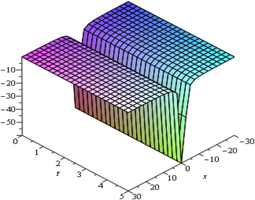
Solitary waves arise due to indirect balance of nonlinear effects with the dispersive effects. From the above graphs, we are able to judge that soliton is a wave which preserves its shape after it strikes with another wave of the similar kind. The waves produced by linear description tend to experience dispersion and create localized disturbance to spread. The solitary waves can intuitively be anticipated to be the outcome of two effects of steepening and spreading with marginally nonlinear amplitude. The waves of various types of wave-number, there speeds and amplitude as they rely upon the process of dispersion being generated without changing their actual shapes. We have observed that media go under strong dispersion process and can generate high amplitude waves and oppositely weak dispersive media generate such waves of small amplitude.

We attain the desired solution through rational functions. The hyperbolic and trigonometric function travelling wave solutions of nonlinear Caudrey-Dodd-Gibbon equation are represented in Figures 1 and 2 respectively for different values of physical parameters. Figures 3 and 4 show soliton solutions for various physical parameters through exponential and rational functions. 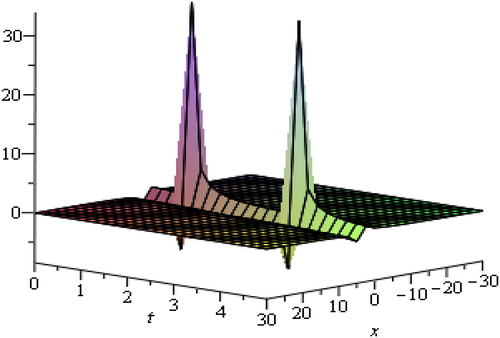Figure 5 shows rational function solution for different values of $\lambda ,\mathrm{ }\mu \mathrm{ }$ and $c_1.$ In these graphical results, it is taken $\beta =30.$ By changing the values of physical and additional free parameters, the velocity and amplitude of solitary waves are controlled. It is observed that the displacement potential $\eta$ becomes sharp at leading and trailing edges. Amplitude is proportional to the velocity of propagation also taller solitary waves are thinner and move faster.

Figure 1. Represents 3 D plot for $\lambda =0.2,\mathrm{ }\mu =1,\mathrm{ }{c}_1=2,\mathrm{ }{a}_0=1,-30\le x\le 30,\mathrm{ }0\le t\le 5.$

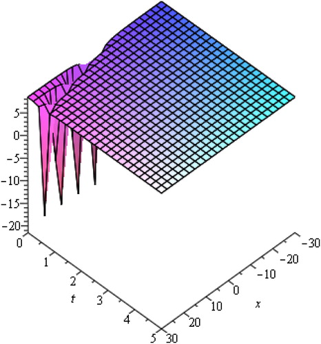
Figure 2. Represents 3 D plot for $\lambda =0.2,\mathrm{ }\mu =1,\mathrm{ }{c}_1=2,\mathrm{ }{a}_0=1,-30\le x\le 30,\mathrm{ }0\le t\le 5.$

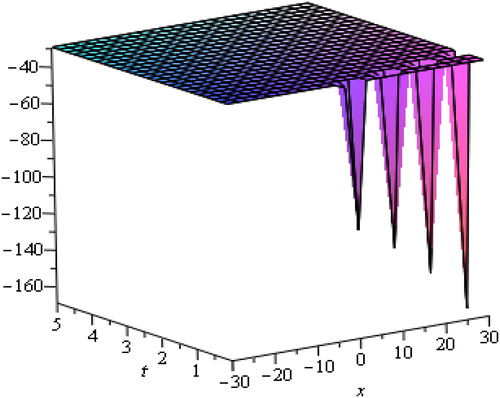
Figure 3. Signifies 3 D plot for $\lambda =1,\mathrm{ }\mu =-1,\mathrm{ }{c}_1=0.1,\mathrm{ }{a}_0=2,-30\le x\le 30,\mathrm{ }0\le t\le 4.$

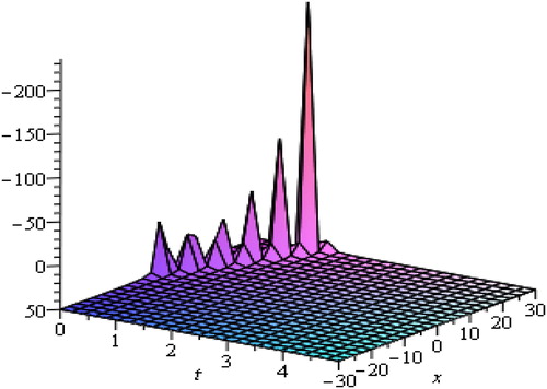
Figure 4. Signifies 3 D plot for $\lambda =1,\mathrm{ }\mu =-1,\mathrm{ }{c}_1=0.1,\mathrm{ }{a}_0=2,-30\le x\le 30,0\le t\le 4.$

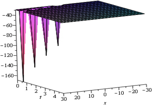
Figure 5. Shows 3 D plot for $\lambda =-1,\mathrm{ }\mu =2,\mathrm{ }{c}_1=1,-30\le x\le 30,0\le t\le 5.$

Next, Figures 6 and 7 show hyperbolic and trigonometric function travelling wave solutions of Pochhammer-Chree (PC) equation respectively by setting suitable values of physical parameters which control the solitary wave amplitude. Also, Figures 8 and 9 show exponential and rational function solutions respectively. Figure 10 shows rational function solution for different values of $\mathrm{a},c_1$ and $b.$ The solitary wave moves toward right if the velocity is positive and left directions if the velocity is negative, and the amplitudes and velocities are controlled by various physical parameters. Solitary waves show more complicated behaviours which are controlled by various physical and additional free parameters. Figures indicate graphical solutions for altered values of physical parameters. Arbitrary functions can be affected by the solitary wave solution. It is concluded that various constraint can be selected as an input to our simulation. Solitary waves for various values of physical and additional free parameters are being pointed out by the graphic illustration. From above discussed graphical cases it has been observed that solution of soliton waves does not rely completely upon the additional free parameters. The soliton waves of different types are clearly described by the graphic outcomes.

Figure 6. Represents 3 D plot for $\lambda =-1,\mathrm{ }\mu =2,\mathrm{ }{c}_1=0.1,a=3,b=1,-30\le x\le 30,\mathrm{ }0\le t\le 5.$

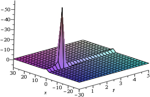
Figure 7. Represents 3 D plot for $\lambda =-1,\mathrm{ }\mu =2,\mathrm{ }{c}_1=0.1,a=3,b=1,-30\le x\le 30,\mathrm{ }0\le t\le 5.$

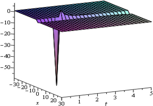
Figure 8. Signifies 3 D plot for $\lambda =1,\mathrm{ }\mu =2,\mathrm{ }a=0.1,c_1=1,b=3,-30\le x\le 30,\mathrm{ }0\le t\le 4.$

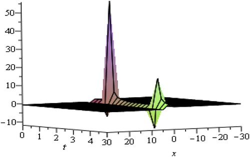
Figure 9. Signifies 3 D plot for $\lambda =1,\mathrm{ }\mu =2,a=0.1,\mathrm{ }{c}_1=1,b=3,-30\le x\le 30,\mathrm{ }0\le t\le 4.$

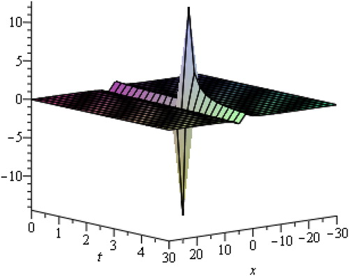
Figure 10. Shows 3 D plot for $a=0.1,\mathrm{ }b=1,\mathrm{ }{c}_1=2,-30\le x\le 30,0\le t\le 4.$

5. Conclusion

In this paper, the main focus is to find, test and analyze the new travelling wave solutions and physical properties of nonlinear Caudrey-Dodd-Gibbon (CDG) and Pochhammer-Chree (PC) equations by applying reliable mathematical technique. It is noted that soliton type solution is allowed by the under study nonlinear differential equation. The applied algorithm is helpful to verify the results that are acquired by the exact solution. The closeness among the outcome discloses that for solving differential equation it behaves like a powerful tool. CDG and PC equations have very important part in solitary wave’s theory as it opens up the various natures of soliton wave solution, and to handgrip these equations we use an expansion technique as a tool which is proper and authentic. The conclusion is very clear to check the physical behaviour of solitary waves, we use valuable way under study method. The method has been applied directly without requiring linearization, discretization or perturbation. The obtained results demonstrate the reliability of the algorithm and give it a wider applicability to nonlinear differential equations. Although using Maple software it permits us more solution sets, less computational work and less computer memory.

Disclosure statement

No potential conflict of interest was reported by the authors.

References

- Abbasbandy, S. (2007). Numerical solutions of nonlinear Klein-Gordon equation by variational iteration method. International Journal for Numerical Methods in Engineering, 70(7), 876–881. doi: 10.1002/nme.1924
- Abdou, M. A. (2007). The extended tanh-method and its applications for solving nonlinear physical models. Applied Mathematics and Computation, 190(1), 988–996. doi: 10.1016/j.amc.2007.01.070
- Akbar, M. A., & Ali, N. H. M. (2012). New Solitary and Periodic Solutions of Nonlinear Evolution Equation by Exp-function Method. World Applied Sciences Journal, 17(12), 1603–1610.
- Akbar, M. A., Ali, N. H. M., & Zayed, E. M. E. (2012). Abundant exact traveling wave solutions of the generalized Bretherton equation via (G′/G)-expansion method. Communications in Theoretical Physics, 57(2), 173–178. doi: 10.1088/0253-6102/57/2/01
- Ali, A. T. (2011). New generalized Jacobi elliptic function rational expansion method. Journal of Computational and Applied Mathematics, 235(14), 4117–4127. doi: 10.1016/j.cam.2011.03.002
- Dai, C. Q., Wang, Y. Y., Fan, Y., & Yu, D. G. (2018). Reconstruction of stability for Gaussian spatial solitons in quintic–septimal nonlinear materials under PT -symmetric potentials. Nonlinear Dynamics, 92(3), 1351–1358. doi: 10.1007/s11071-018-4130-4
- Ding, D. J., Jin, D. Q., & Dai, C. Q. (2017). Analytical solutions of differential difference Sine- Gordon equation. Thermal Science, 21(4), 1701–1705. doi: 10.2298/TSCI160809056D
- Feng, G., Yang, X. J., & Srivastava, H. M. (2017). Exact Travelling wave solutions for linear and nonlinear heat transfer equations. Thermal Science, 21(6), 2307–2311. doi: 10.2298/TSCI161013321G
- He, J. H., & Wu, X. H. (2006). Exp-function method for nonlinear wave equations. Chaos, Solitons & Fractals, 30, 700–708. doi: 10.1016/j.chaos.2006.03.020
- Hirota, R. (1973). Exact envelope soliton solutions of a nonlinear wave equation. Journal of Mathematical Physics, 14(7), 805–810. doi: 10.1063/1.1666399
- Hirota, R., & Satsuma, J. (1981). Soliton solution of a coupled KdV equation. Physics Letters A, 85(8–9), 407–408. doi: 10.1016/0375-9601(81)90423-0
- Hu, H., & Li, Y. (2018). New interaction solutions and nonlocal symmetries for the (2 + 1)-dimensional coupled Burgers equation. Arab Journal of Basic and Applied Sciences, 25(2), 71–76. doi: 10.1080/25765299.2018.1449417
- Inc, M., & Evans, D. J. (2004). On travelling wave solutions of some nonlinear evolution Equations. International Journal of Computer Mathematics, 81(2), 191–202. doi: 10.1080/00207160310001603307
- Islam, M. T., Akbar, M. A., & Azad, M. A. K. (2017). Multiple closed form wave solutions to the KdV and modified KdV equations through the rational (G′/G)-expansion method. Journal of the Association of Arab Universities for Basic and Applied Sciences, 24(1), 160–168. doi: 10.1016/j.jaubas.2017.06.004
- Khan, K., & Akbar, M. A. (2013). Application of exp (−φξ)-expansion Method to find the Exact Solutions of Modified Benjamin-Bona-Mahony Equation. World Applied Sciences Journal, 24(10), 1373–1377.
- Kaplan, M., & Akbulut, A. (2018). Application of two different algorithms to the approximate long water wave equation with conformable fractional derivative. Arab Journal of Basic and Applied Sciences, 25(2), 77–84. doi: 10.1080/25765299.2018.1449348
- Liping, W., Senfa, C., & Chunping, P. (2009). Travelling wave solution for Generalized Drinfeld-Sokolov equations. Applied Mathematical Modelling, 33, 4126–4130.
- Saad, K. M., Al-Shareef, E. H., Mohamed, M. S., & Yang, X. J. (2017). Optimal q-homotopy analysis method for time-space fractional gas dynamics equation. The European Physical Journal Plus, 132(1), 11303–11306. doi: 10.1140/epjp/i2017-11303-6
- Shehata, A. R. (2010). The travelling wave solutions of the perturbed nonlinear Schrodinger equation and the cubic-quintic Ginzburg Landau equation using the modified (G′/G)-expansion method. Applied Mathematics and Computation, 217(1), 1–10. doi: 10.1016/j.amc.2010.03.047
- Sirendaoreji. (2004). New exact travelling wave solutions for the Kawahara and modified Kawahara equations. Chaos, Solitons & Fractals, 19, 147–150.
- Wang, M. (1995). Solitary wave solutions for variant Boussinesq equations. Physics Letters A, 199(3–4), 169–172. doi: 10.1016/0375-9601(95)00092-H
- Wang, M., Li, X., & Zhang, J. (2008). The (G′/G)-expansion method and travelling wave solutions of nonlinear evolution equations in mathematical physics. Physics Letters A, 372(4), 417–423. doi: 10.1016/j.physleta.2007.07.051
- Wang, Y. Y., Chen, L., Dai, C. Q., Zheng, J., & Fan, Y. (2017). Exact vector multipole and vortex solitons in the media with spatially modulated cubic–quintic nonlinearity. Nonlinear Dynamics, 90(2), 1269–1275. doi: 10.1007/s11071-017-3725-5
- Wang, Y. Y., Dai, C. Q., Xu, Y., Q., Zheng, J., & Fan, Y. (2018). Dynamics of nonlocal and localized spatiotemporal solitons for a partially nonlocal nonlinear Schrödinger equation. Nonlinear Dynamics, 92(3), 1261–1269. doi: 10.1007/s11071-018-4123-3
- Wang, Y. Y., Zhang, Y. P., & Dai, C. Q. (2016). Re-study on localized structures based on variable separation solutions from the modified tanh-function method. Nonlinear Dynamics, 83(3), 1331–1339. doi: 10.1007/s11071-015-2406-5
- Wazwaz, A. M. (2004). A sine-cosine method for handing nonlinear wave equations. Mathematical and Computer Modeling, 40(5-6), 499–508. doi: 10.1016/j.mcm.2003.12.010
- Weiss, J., Tabor, M., & Carnevale, G. (1983). The Painleve property for partial differential equations. Journal of Mathematical Physics, 24(3), 522–526. doi: 10.1063/1.525721
- Yang, X. J. (2016). A New integral transform method for solving steady Heat transfer problem. Thermal Science, 20(suppl. 3), 639–S642. doi: 10.2298/TSCI16S3639Y
- Yang, X. J., & Feng, G. (2017). A New Technology for Solving Diffusion and Heat Equations. Thermal Science, 21(1 Part A), 133–140. doi: 10.2298/TSCI160411246Y
- Yang, X. J., Feng, G., & Srivastava, H. M. (2017). Exact travelling wave solutions for the local fractional two-dimensional Burgers-type equations. Computers & Mathematics with Applications, 73(2), 203–210. doi: 10.1016/j.camwa.2016.11.012
- Yang, X. J., Tenreiro Machado, J. A., Baleanu, D., & Cattani, C. (2016). On exact traveling wave solutions for local fractional Korteweg-de Vries equation. Chaos: An Interdisciplinary Journal of Nonlinear Science, 26(8), 084312. doi: 10.1063/1.4960543
- Zayed, E. M. E. (2010). Traveling wave solutions for higher dimensional nonlinear evolution equations using the (G′/G)-expansion method. Journal of Applied Mathematics & Informatics, 28, 383–395.
- Zayed, E. M. E., & Gepreel, K. A. (2009). The (G′/G)-expansion method for finding the traveling wave solutions of nonlinear partial differential equations in mathematical physics. Journal of Mathematical Physics, 50, (1), 013502–013514. doi: 10.1063/1.3033750
- Zayed, E. M. E., & Al-Nowehy, A. G. (2017). The solitary wave ansatz method for finding the exact bright and dark soliton solutions of two nonlinear Schrödinger equations. Journal of the Association of Arab Universities for Basic and Applied Sciences, 24(1), 184–190. doi: 10.1016/j.jaubas.2016.09.003
- Zayed, E. M. E., Zedan, H. A., & Gepreel, K. A. (2004). On the solitary wave solutions for nonlinear Hirota-Satsuma coupled KdV equations. Chaos, Solitons & Fractals, 22, 285–303. doi: 10.1016/j.chaos.2003.12.045
- Zhang, J., Jiang, F., & Zhao, X. (2010). An improved (G′/G)-expansion method for solving nonlinear evolution equations. International Journal of Computer Mathematics, 87(8), 1716–1725. doi: 10.1080/00207160802450166
- Zhang, F., Qi, J. M., & Yuan, W. J. (2013). Further Results about Traveling Wave Exact Solutions of the Drinfeld-Sokolov Equations. Journal of Applied Mathematics, 2013, 1–6. doi: 10.1155/2013/523732