Hoist scheduling for an anodizing plant at an extrusion company

Abstract

The field of scheduling metal surface treatment plants is extensively studied in the literature and it is referred to by the name of Hoist Scheduling Problem (HSP). HSP is classified as a flow-shop scheduling problem, but differs because of the transportation constraints and the no-wait restriction. This research deals with a real anodizing plant in an extrusion company with multiple-hoist. The objective of this study is to minimize the makespan of a demand of selected days and to improve production of the plant. A heuristic algorithm was developed for scheduling the anodizing demand of the extrusion company. The algorithm was coded in Matlab (R2015b – editor) to simulate the production of certain days. The runs of the simulation were divided into three phases: validation phase; experimentation phase; and productivity enhancement phase. The results showed a reduction in the makespan with an approximated average of 18%. Furthermore, it revealed that the algorithm was able to utilize the time by an approximated average of 98% and to increase the number of jobs by an approximated average of 20%.

Keywords:

• Anodizing plant
• heuristic algorithm
• hoist scheduling problem
• makespan minimization

1. Introduction

Scheduling of automated metal surface treatment plants like electroplating, printed circuit board and anodizing are referred in the literature by “Hoist Scheduling Problem (HSP)”. Where one hoist or more are assigned to transport jobs from one stage to another stage while respecting the treatment durations in each stage. Even though hoist scheduling problems are extensively studied in the literature, they are still under development to meet other criteria and to find better and faster algorithms.

In this research, a real anodizing plant is studied. In this plant, a number of different profiles (jobs) are dipped in a series of tanks that are filled with acids, water, dyes and other chemicals for varying lengths of time. The transportation of these jobs from one tank to another is done by five hoists (cranes) with overlapping movement ranges. The purpose of the study is minimizing the makespan, and use the remaining time to treat more jobs, thus, increasing the production as well.

The anodizing plant is composed of 60 positions arranged into two parallel sides that are linked by two transferors. The positions are grouped to form 27 stages as listed in Table 1. Such scheduling problem is referred in the literature by the term multi-capacity problem (Bloch, Manier, Baptiste, & Varnier, 2010). Moreover, some products’ recipes requires the profiles to be treated twice in some tanks, others skip some stages. Therefore, this problem is known as multi-product (Bloch et al., 2010).

Table 1. Stages of the anodizing plant.

Stage no.	Stage Name	Side	Stage no.	Stage Name	Side
1	Outside	1	15	Desmutting Rinsing 1	2
2	Loading	1	16	Desmutting Rinsing 2	2
3	Input Buffers Zone 1	1	17	Anodizing	2
4	Transferor 1	1 & 2	18	Anodizing Rinsing 1	2
5	Input Buffers Zone 2	2	19	Anodizing Rinsing 2	2
6	Alkaline	2	20	Transferor 2	2 & 1
7	Alkaline Rinsing	2	21	Electro-Coloring	1
8	Etching	2	22	Electro-Coloring Rinsing 1	1
9	Etching Rinsing 1	2	23	Electro-Coloring Rinsing 2	1
10	Etching Rinsing 2	2	24	Demi-Rising	1
11	Etching Rinsing 3	2	25	Hot Sealing	1
12	Etching Rinsing 4	2	26	Output Buffers Zone	1
13	Etching Rinsing 5	2	27	Unloading	1
14	Desmutting	2

The five shaded stages in Table 1 are waiting stages.

This article is composed of eight sections, in the introduction, a background of the study, brief description of the plant along with the objectives are mentioned. In the second section, the hoist scheduling problems and similar previous studies are reviewed. In the third section, the methodology is introduced followed by a description of the collected data and the construction of the simulation model. A mathematical model is proposed in the fourth section that describes the time events and constraints. Some of these constraints are used in the algorithm, which are explained in the fifth section. The results undergo through phases of validation and experimentations, these results are discussed in the sixth and the seventh sections. Finally, in the eighth section, a conclusion, and few recommendations are given as well as topics that are left for further studies that will help in improving the algorithm even better.

2. Literature review

A Dynamic Hoist Scheduling Problem (DHSP) with multi-items for four different types of anodizing plants was studied by Paul, Bierwirth, and Kopfer (2007). They used a heuristic algorithm named Adaptive Time Window (ATW), which corrects the violations by back-tracking to previous stages as well as previous jobs. They claim that their ATW algorithm is expected to increase the production by 20%, if it is implemented in a real plant. One research that studied an anodizing plant similar to the plant chosen for this study is for a Danish company named Bang and Olufsen (Skov, 2007). Two approaches were adopted; the first one simulates the scheduling scheme implemented by the company, while the second one considers the No-Wait constraints via applying meta-heuristics using the Alternative Graph Model. The drawback of the simulation model is that can backtrack to one previous stage to correct the violation.

Liu, Zhao, and Xu (2012) worked on a real electroplating process, and used a Mixed-Integer Dynamic Optimization (MIDO) model along with an algorithm to optimize three objectives: minimizing the makespan, energy consumption and fresh/waste water of the rinsing tanks. Elmi and Topaloglu (2013) employed Taguchi’s methods to experiment for different levels (number) of part types, stages and robots. Their problem, which also has multi-machines per stage, is solved by a Simulated Annealing (SA) algorithm. This algorithm to some extent similar to the algorithm of this research. However, because of the Time Window (TW) constrains, violations can be avoided by releasing some jobs earlier, minding the TW constraints.

El Amraoui, Manier, El Moudni, and Benrejeb (2013) adopted a Genetic Algorithm (GA) to minimize the cyclic time for their single-hoist, multi-product problem. For a maximum population of 10 jobs and using the algorithm with two operators, two-point crossover and swapping mutation, they are able to achieve a short cycle time of less than 16 min. Mateo Doll, Manier, and Companys Pascual (2015) compared the results of their Branch-and-Bound (B&B) algorithm with the results by El Amraoui et al. (2013). Their algorithm is able to produce the same cycle times of El Amaroui’s but in much faster computational time.

Another research conducted on an anodizing plant is on a plant in Thailand by Pantusavase and Hassamontr (2015), they developed an algorithm to minimize the cycle time for a mixed loads sequence. Feng, Che, and Chu (2015) improved a Mixed Integer Programming (MIP) to deal with a complicated case of DHSP that has multiple capacity machines. Their DHSP minimizes the makespan for three types of jobs, using one hoist only.

Elmi and Topaloglu (2017) solved a multi-degree cyclic problem with two robots using a Mixed-Integer Linear Programming (MILP) model. They optimized the number of robots and the number of cycles. However, they ignored the robot collision constraints, as they did in their 2013 study. Che, Kats, and Levner (2017) investigated a bi-criteria optimization problem to minimize the cycle time and maximize the stability radius. They used a parametric critical path algorithm with complexity of O(m⁴), where m is the number of machines.

Basán, Pulido, Cóccola, and Méndez (2017) developed a heuristic strategy for requesting the hoist based on the time window slots of the job recipe and the job priority. Their proposed strategy is capable of generating near-optimal schedules to achieve their aim of reducing the makespan and cost for many scenarios in a short time period. A Hybrid Quantum Evolutionary Algorithm (QEA) is developed by Lei, Manier, Manier, and Wang (2017) that combines two types of decoding schemes (binary-decimal decoding and shifting decoding) to write their genetic algorithm for their single-hoist CHSP. Lei’s algorithm shows the same cycle times obtained by the CPLEX with faster computational time. On the other hand, it gives better cycle times than the previous studies, but with slower computational time.

To sum up, the HSP is considered one of the hardest scheduling problems, especially when the processing times are short (short-limit) (Basán et al., 2017). Some HSPs can be so complex that they are classified as NP-hard problems to the extent that some of them are impossible to solve (Skov, 2007). However, there are several Heuristic algorithms that are capable of finding a reasonable solution, and when they are combined with other algorithms they might give a better solution. Another way to deal with such complex problems is to solve them by graphical simulation program rather than analytically (Basán et al., 2017). Moreover, the algorithms in the field of HSP are exhibiting a huge improvements like the study by Lei et al. (2017), and dealing with multi-objectives like the study by Liu et al. (2012) and Feng et al (2015). However, the simulated plants in the recent studies are still lacking additional characteristics that make their plants mimic real complex plants, such as multi-hoist, multi-capacity tanks, loading stations, unloading stations and buffers.

In this study, a heuristic algorithm is used to minimize the makespan for a real anodizing plant with multi-hoist, multi-product, multi-capacity tanks, loading stations, unloading stations, and input and output buffers. Different combinations of jobs’ sequences and tanks’ configurations are examined for their effect on the makespan and their effect on improving the performance of two stages, namely, the Hot Sealing stage, and the Anodizing stage. Therefore, this study considers the design aspect in term of the tanks configurations, and the scheduling aspect in term of job sequences.

3. Methodology

3.1. Introduction to the methodology

The methodology adopted in this research is theoretical, where a simulated version of the actual plant is mathematically modelled by the description of the time events and constraints, then it is solved using a heuristic algorithm. Historical production data of twelve days are used to validate the algorithm. After that, experimentations with the algorithm are carried out.

The plant is simulated to develop the schedule and to conduct some experimentations which are difficult to be carried out in the real plant.

3.2. The simulation model and relaxations

The context of the problem in this research is considered to be a Predictive Hoist Scheduling Problem (PHSP), because the list of the jobs that to be scheduled are already given along with their recipes and do not arrive randomly.

The simulation model in this research has the following relaxations made to the actual plant:

1. There is no consideration for the breakdown and maintenance, and it is assumed that all of the 60 positions are available all the time and the hoists do not jam.

2. The number of carriers is assumed to be infinite; therefore, each job has its own carrier.

3. All empty hoist moves are assumed to have a fixed duration of 20 sec before every loaded hoist move.

4. Selection of the hoist in the overlap zones is based on the hoist with the higher number not the closest hoist to the position at which the finished job is located. For example, if a job finished in a position located in the overlap zone between hoist 2 and 3, then hoist 3 is selected, even if hoist 2 was the hoist nearest to that position. This is because of the difficulty faced in tracking the hoists movements.

3.3. Collection of historical data

The number of days selected for this study is twelve (12) days, three of them are from April 2015 and the other nine are from February and June 2017. These twelve days are chosen out from around 50 days from these months. Each day consists of two shifts of operation (16 hours), where the operations start with prepared jobs from the previous day, already placed in the Loading, the Input Buffers and the Outside stages.

The reasons of selecting these 12 days are based on the number of produced jobs and their variety. Each day had a variety of recipes and the number of jobs is 45 or more, which is anticipated of less breakdown times. The data used in this study are extracted from the anodizing tanks daily reports which are log sheets that include the number, the proprieties of the jobs and the starting and finishing times at the anodizing stage.

3.4. Construction of the simulation runs

The simulation runs are divided into three phases: validation, experimentation and further experimentation.

Each run is defined by the day number and the combination used, which is defined by the method of jobs’ sequencing and the tanks’ configuration as it is illustrated in Table 2.

Table 2. The nine combinations.

	Configuration 1 (C1)	Configuration 2 (C2)	Configuration 3 (C3)
Sequence 1 (S1)	Combination 1 (S1C1)	Combination 2 (S1C2)	Combination 3 (S1C3)
Sequence 2 (S2)	Combination 4 (S2C1)	Combination 5 (S2C2)	Combination 6 (S2C3)
Sequence 3 (S3)	Combination 7 (S3C1)	Combination 8 (S3C2)	Combination 9 (S3C3)

3.4.1. Sequences

The sequence of the jobs is the order in which the jobs enter the first chemical treatment (Alkaline). In this study, three types of jobs’ sequencing methods are used in the simulation model. Sequence 1 (The Actual Sequence), which is the sequence used for the actual data; Sequence 2 (Lowest Recipe Identification (ID) First (LRIDF)), which orders the jobs entering the Alkaline stage in ascending order of their recipe ID. Sequence 3 (Highest Recipe Identification (ID) First (HRIDF)), which orders the jobs entering the Alkaline stage in descending order of their recipe ID.

3.4.2. Configurations

Three configurations are simulated that are concerned with the number of tanks in the Anodizing stage and the Hot Sealing stage. Configuration 1 is the Actual Configuration; Configuration 2 has one extra anodizing tank and one extra hot sealing tank; and Configuration 3 has one extra anodizing tank and two extra hot sealing tanks. The extra anodizing tank will replace a rinsing tank (position 36) while the extra hot sealing tanks will replace two output buffers (positions 47 and 48). Thus, the number of positions is kept 60 positions.

3.4.3. Combinations

The stated three jobs’ sequences and three tanks’ configurations form nine combinations illustrated in Table 2. For example, Sequence 1 and Configuration 2 give Combination 2 (S1C2).

4. Mathematical model formulation

4.1. Notations

The notations used in the mathematical model are slightly different from the notations used later in the algorithm equations. The reasons for this is because the mathematical model covers the whole model without the relaxations regarding the empty hoist movements and the hoists assignments. While in the algorithm, the empty hoists movements and the hoist assignments are not expressed mathematically, but they are replaced with alternative methods.

Events: There are four operations; each has a starting event and finishing event: $$OE=\{PS/PF/LS/LF/ES/EF/WS/WF\}$$ where $PS:$ Process (Treatment) Start; $PF:$ Process (Treatment) Finish; $LS:$ Loaded hoist move Start; $LF:$ Loaded hoist move Finish; $ES:$ Empty hoist move Start; $EF:$ Empty hoist move Finish; $WS:$ Waiting hoist Start; $WF:$ Waiting hoist Finish. The waiting hoist is an empty hoist but in a stop condition.

The Notations used for the time indicator of treatment or loaded hoist move are: $$T_{p,i,r,(s/ns),(k/v)}^{OE,h}$$ where $T:$ Time indicator; $OE$ (Operation Event): PS, PF, LS, LF; $h:$ Hoist no. used; $p:$ Job priority of the current job; $i:$ Job ID of the current job; $r:$ Recipe ID of the current job; $s/ns:$ current stage/next stage; $k/v:$ current position (known)/next position (known).

The Notations used for the time indicator of an empty hoist move or a waiting hoist are: $$t_{(k/c)}^{OE,h}$$ where $t:$ time indicator; $OE$ (Operation Event): ES, EF, WS, WF; $h:$ Hoist no. used; $k/c:$ destination position (known)/current (initial) position (unknown).

In addition, the following notations are defined:

Jobs: $i=(1,2,3,\dots ,n),$ where $n$ is the last priority job.

Recipes: $r=\left\{1,2,3,\dots ,30\right\},$ there are 30 recipes.

Stage: $s/ns=(1,\mathrm{ }2,\mathrm{ }3,\dots ,\mathrm{ }27),$ where $27$ is the last stage (unloading) for all the recipes, yet some of the stages are skipped for some recipes.

Position: $k/v=\{1,\mathrm{ }2,\mathrm{ }3,\dots .,\mathrm{ }60\},$ there are 60 positions.

The next position ($v$) depends on two variables: the recipe type and the next stage, i.e. $v=f(r\_\mathit{type},ns).$

Hoist: There are 5 physical hoists; the sixth hoist is an imaginary hoist that carries the jobs from Outside stage to the Loading stage

$$h=\{1/2/3/4/5/6\}$$

The ranges of the hoists are expressed as below: $$\mathrm{For} h=1: \left(2\le k\le 8 \right) \mathrm{and} \left(47\le k\le 60 \right);h=2: \left(9\le k\le 27 \right);$$ $$h=3:\left(23\le k\le 30 \right);h=4:\left(28\le k\le 37 \right);h=5: \left(38\le k\le 57 \right).$$

Overlaps between hoists ranges are necessary to transport the jobs from the beginning to the end of the anodizing line, which implies attention to avoid hoists collision during simulating the production.

The notations for the operations’ durations are as follows:

$d_{r,s}^P$ is the treatment duration of the $s$ th stage for recipe ($r$).

$d_{k\to v}^{L,h}$ is the duration for the loaded hoist ($h$) to move from the current position ($k$) to the next position ($v$).

$d_{c\to k}^{E,h}$ is the duration to move the empty hoist ($h$) from the position ($c$) to the destination position ($k$).

$d_k^{W,h}$ is the waiting duration for the hoist ($h$) waiting above position ($k$).

4.2. The mathematical model

The objective function is to minimize the make-span expressed in Equation (4.1)(4.1) $$C_{\mathit{max}}=\underset{\forall \mathit{Possible} \mathit{Sequnces} }{\min }\left(\underset{\forall i}{\max } \left(T_{n,i,r,27,k}^{PF,h}\right)\right)$$(4.1) . That means to minimize the duration to complete all the jobs of one day through all stages. In other words, minimizing the finishing time of the last job at the last stage, which is the maximum finishing time among all the jobs. (4.1) $$C_{\mathit{max}}=\underset{\forall \mathit{Possible} \mathit{Sequnces} }{\min }\left(\underset{\forall i}{\max } \left(T_{n,i,r,27,k}^{PF,h}\right)\right)$$(4.1) where $C_{\mathit{max}}$ is the makespan, i.e. the job with the maximum finishing time at the last stage.

The possible job sequences are set to be the tuning parameter (changing the jobs priorities) to obtain the minimum makespan. Another tuning parameter is testing all the alternative hoists movements, but it is not considered due to its complexity.

The objective function is subject to the following constraints (4.2) $$T_{p,i,r,s,k}^{PF}=T_{p,i,r,s,k}^{PS}+d_{r,s}^P$$(4.2) (4.3) $$t_k^{\left(E/W\right)F,h}\le T_{p,i,r,s,k}^{PF}$$(4.3) (4.4) $$t_k^{\left(E/W\right)F,h}=\left\{\begin{array}{l}{t}_k^{EF,h}\mathit{\text{ if it is }}\mathit{perferred}\mathit{\text{ to }}\mathit{move} \mathit{the} \mathit{empty} \mathit{hoist} \\ t_k^{WF,h}\mathit{\text{ if it is }}\mathit{perferred}\mathit{\text{ to }}\mathit{make} \mathit{the} \mathit{empty} \mathit{hoist} \mathit{wait} \end{array}\right.$$(4.4) (4.5) $${ t}_k^{WF,h}=t_k^{WS,h}+d_k^{W,h}$$(4.5) (4.6) $${ t}_{\mathrm{k}}^{EF,h}=t_c^{ES,h}+d_{c\to k}^{E,h}$$(4.6) (4.7) $$t_k^{WS,h}=\left\{\begin{array}{l}{T}_{p,i,r,s,k}^{LF,h}\mathit{\text{ if }}\mathit{the} \mathit{hoist} \left(h\right) \mathit{has} \mathit{just} \mathit{loaded} \\ a \mathit{job at position} \left(k\right) \\ t_k^{EF,\left(h/h^{\mathrm{\prime }}\right)}\mathit{\text{ if }}\mathit{the} \mathit{empty} \mathit{hoist} \left(h\right)\mathit{\text{has }}\mathit{just} \\ \mathit{moved to position} \left(k\right)\end{array}\right.$$(4.7) (4.8) $$t_k^{EF,\left(h/h^{\mathrm{\prime }}\right)}=\underset{\forall h}{\min }(t_c^{ES,h}+d_{c\to k}^{E,h}, t_{c^{\mathrm{\prime }}}^{ES,h^{\mathrm{\prime }}}+d_{c^{\mathrm{\prime }}\to k}^{E,h^{\mathrm{\prime }}})$$(4.8) (4.9) $$t_c^{ES,h}=\left\{\begin{array}{l}{t}_c^{WF,h}\mathit{\text{ if }}\mathit{the} \mathit{empty} \mathit{hoist} \left(h\right) \mathit{has} \mathit{ended} \\ \mathit{waiting from position} \left(c\right) \\ T_{p^{\mathrm{\prime }},i^{\mathrm{\prime }},r^{\mathrm{\prime }},s^{\mathrm{\prime }}c}^{LF,h}\mathit{\text{ if }}\mathit{the} \mathit{hoist} \left(h\right)\mathit{\text{has }}\mathit{just} \mathit{loaded} \\ a \mathit{job at position} \left(c\right) \end{array}\right.$$(4.9) (4.10) $$t_c^{\left(E/W\right),h}=T_{p,i,r,s,k}^{PF}- d_{c\to k}^{\left(E/W\right),h}$$(4.10) (4.11) $$T_{p,i,r,s,k}^{LS,h}=T_{p,i,r,s,k}^{PF}$$(4.11) (4.12) $$T_{p,i,r,s,v}^{LF,h}=T_{p,i,r,s,k}^{LS,h}+\mathit{pickup} \mathit{duartion}+d_{k\to v}^{L,h}+\mathit{dipping} \mathit{duartion}$$(4.12) (4.13) $$T_{p,i,r,ns,v}^{PS}=T_{p,i,r,s,v}^{LF,h}$$(4.13) (4.14) $$T_{p,i,r,s,k}^{PS}>T_{p^{\mathrm{\prime }},i^{\mathrm{\prime }},r^{\mathrm{\prime }},s^{\mathrm{\prime }},k^{\mathrm{\prime }}}^{PF}, \mathit{For} \mathit{all} i$$(4.14) (4.15) $$T_{p,i,r,s,k}^{LS,h^{\mathrm{\prime }}}>T_{p^{\mathrm{\prime }},i^{\mathrm{\prime }},r^{\mathrm{\prime }},s^{\mathrm{\prime }},k^{\mathrm{\prime }}}^{LF,h}+d_{k^{\mathrm{\prime }}\to k}^{E,h}$$(4.15) (4.16) $$t_k^{\left(LS/ES\right),h}>t_{k^{\mathrm{\prime }}}^{\left(LS/LF/ES/EF\right),h^{\mathrm{\prime }}}, \mathit{where} k^{\mathrm{\prime }}\ne k-1/k/k+1$$(4.16) (4.17) $$t_v^{\left(LF/EF\right),h}>t_{v^{\mathrm{\prime }}}^{\left(LS/LF/ES/EF\right),h^{\mathrm{\prime }}}, \mathit{where} v^{\mathrm{\prime }}\ne v-1/v/v+1$$(4.17)

Equations (4.2)(4.2) $$T_{p,i,r,s,k}^{PF}=T_{p,i,r,s,k}^{PS}+d_{r,s}^P$$(4.2) , (4.11)(4.11) $$T_{p,i,r,s,k}^{LS,h}=T_{p,i,r,s,k}^{PF}$$(4.11) , (4.12)(4.12) $$T_{p,i,r,s,v}^{LF,h}=T_{p,i,r,s,k}^{LS,h}+\mathit{pickup} \mathit{duartion}+d_{k\to v}^{L,h}+\mathit{dipping} \mathit{duartion}$$(4.12) and (4.13) are related to the job process route, which consists of treatment operations and loaded hoist operations. The reason why these equations are expressed as equalities not as inequalities, is because the treatment durations are fixed (No-wait constraints). This also means that jobs have to move to the next stage as soon as they finish the treatment in the current stage, thus, maintaining the same quality. The empty hoist operations are expressed by Equations (4.3)–(4.10). Equations (4.14)(4.14) $$T_{p,i,r,s,k}^{PS}>T_{p^{\mathrm{\prime }},i^{\mathrm{\prime }},r^{\mathrm{\prime }},s^{\mathrm{\prime }},k^{\mathrm{\prime }}}^{PF}, \mathit{For} \mathit{all} i$$(4.14) and (4.15)(4.15) $$T_{p,i,r,s,k}^{LS,h^{\mathrm{\prime }}}>T_{p^{\mathrm{\prime }},i^{\mathrm{\prime }},r^{\mathrm{\prime }},s^{\mathrm{\prime }},k^{\mathrm{\prime }}}^{LF,h}+d_{k^{\mathrm{\prime }}\to k}^{E,h}$$(4.15) are inequalities that address the blocking constraints for a treatment operation and a loaded hoist operation, respectively. The blocking constraints simply state that a current job cannot be placed in a position or moved by a hoist until the position or the hoist is done with the previous job. The constraints that prevent hoists collision are illustrated by simplified inequalities in Equations (4.16)(4.16) $$t_k^{\left(LS/ES\right),h}>t_{k^{\mathrm{\prime }}}^{\left(LS/LF/ES/EF\right),h^{\mathrm{\prime }}}, \mathit{where} k^{\mathrm{\prime }}\ne k-1/k/k+1$$(4.16) and (4.17)(4.17) $$t_v^{\left(LF/EF\right),h}>t_{v^{\mathrm{\prime }}}^{\left(LS/LF/ES/EF\right),h^{\mathrm{\prime }}}, \mathit{where} v^{\mathrm{\prime }}\ne v-1/v/v+1$$(4.17) , where Equation (4.16)(4.16) $$t_k^{\left(LS/ES\right),h}>t_{k^{\mathrm{\prime }}}^{\left(LS/LF/ES/EF\right),h^{\mathrm{\prime }}}, \mathit{where} k^{\mathrm{\prime }}\ne k-1/k/k+1$$(4.16) is for the position in which the job finished a treatment, while Equation (4.17)(4.17) $$t_v^{\left(LF/EF\right),h}>t_{v^{\mathrm{\prime }}}^{\left(LS/LF/ES/EF\right),h^{\mathrm{\prime }}}, \mathit{where} v^{\mathrm{\prime }}\ne v-1/v/v+1$$(4.17) is for the next position for that job. The hoist collision constraints prevent the gap between any two hoists from being 1 position or less.

5. The scheduling algorithm

As it was explained in Sub-section 3.2, the scheduling type for the problem in this study is PHSP, because the jobs list with their recipes are given. A simple heuristic algorithm is chosen to schedule the jobs of a specific period for minimum makespan without consideration of breakdowns.

The algorithm is mainly composed of two loops, as seen in Figure 1. The outer loop is for identifying and scheduling each job individually (i.e. the current job alone). While the inner loop is for setting the times for the current stage and the next stage as well, so that the availability of the next stage is checked using the blocking constraints. Whenever the job encounters a violation, then the action taken is to return the job to the last visited waiting stage (stages that severs as checkpoints where extra durations are allowed, even if the required treatment duration is over), where its leaving time is delayed for 20 sec. In-addition, the job history is removed from three main matrices: BlockPosition ($\mathit{BP}$), HoistCarryJob ($\mathit{HCJ}$) and BlockHoist ($\mathit{BH}$). In other words, it means to unblock the durations of the violated job from last visited waiting stage to the stage where the violation happened, this includes the empty move preceding the time at which the job left this last waiting stage. Then the algorithm tries another schedule until the job is successfully scheduled. On the other hand, if the job does not encounter a violation, then it will simply continue to the next stage, until all its stages are successfully scheduled. This procedure is repeated for the remaining jobs.

Figure 1. Simplified structure of the scheduling algorithm.

Selecting less than 20 sec for the delay duration may produce better results; however, it is fixed to 20 sec to speed-up the computational time of the algorithm while maintaining it around the duration of the hoist pick-up time. The delay action is applied for any type of violation (i.e. the unavailability of the positions/hoists or the possibility of hoists collision).

The Algorithm is coded using Matlab R2015b editor and run using an Intel (R) Core (TM) processor with a speed of (2.00 GHz to 2.60 GHz) and a RAM memory size of 8.00 GB. The reason for coding with Matlab editor is to create three main matrices that will act as platforms for the scheduling procedure. The first one named BlockPosition ($\mathit{BP}$), which has two-dimensions of (position no. vs. time), it is used to block positions with Job-ID. The other two are for the hoists, each with two-dimensions of (hoist no. vs. time). One is used to block the hoist to a job by its Job-ID, it is named HoistCarryJob ($\mathit{HCJ}$), whereas the second is used to block the hoist to its current position ($k$) and next position ($v$), it is named BlockHoist ($\mathit{BH}$).

Other matrices that act as input data are four:

1. The Treatment Duration matrix ($\mathit{DT}$): treatment duration for a given recipe ($r$) and current stage ($s$) is taken from $DT \left(r,s\right).$

2. The Loaded Hoist Duration matrix ($\mathit{DHL}$): loaded hoist duration from a given current position ($k$) to a given next position ($v$) for the current job is taken from $\mathit{DHL} (k,v).$

3. The Possible Positions matrix ($\mathit{PP}$): this matrix is used to check if the next position in the next stage ($ns$) for a given recipe type ($r\_\mathit{typer}$) is available. In case all positions of the next stage are busy, then the job is returned to the last visited stage and delayed.

4. The Job Properties matrix, which is a list of strings describing the properties of the job: $\mathit{i}$ for $\mathbf{Job}-\mathbf{ID}, \mathit{r}$ for$\mathit{recipe} \mathit{ID}$ and$\mathit{p}$ for$\mathit{priority},$ including the starting/current stage and the starting/current position.

Four events matrices $\mathit{TPS},$ $\mathit{TPF},$ $\mathit{TLS}$ and $\mathit{TLF}$ are defined by equations similar to Equations (4.13)(4.13) $$T_{p,i,r,ns,v}^{PS}=T_{p,i,r,s,v}^{LF,h}$$(4.13) , (4.2)(4.2) $$T_{p,i,r,s,k}^{PF}=T_{p,i,r,s,k}^{PS}+d_{r,s}^P$$(4.2) , (4.11)(4.11) $$T_{p,i,r,s,k}^{LS,h}=T_{p,i,r,s,k}^{PF}$$(4.11) and (4.12)(4.12) $$T_{p,i,r,s,v}^{LF,h}=T_{p,i,r,s,k}^{LS,h}+\mathit{pickup} \mathit{duartion}+d_{k\to v}^{L,h}+\mathit{dipping} \mathit{duartion}$$(4.12) , respectively. The equations of the four main events in the mathematical model are transformed into the form of matrices’ elements, to suit the algorithm code, which are given in Equations (5.1)–(5.4). The purpose of these matrices is to record the time of the events and set them for the blocking check-up procedure. (5.1) $$\mathit{TPS} (p,s)=\left\{\begin{array}{l}20 \mathit{seconds},\mathit{\text{ if }}\mathit{the} \mathit{current} \mathit{stage}\mathit{\text{ is }}\mathit{the} \mathit{starting} \mathit{stage} \\ \mathit{\text{TLF }}\left(p,s\mathrm{\prime }\right),\mathit{\text{ if }}\mathit{the} \mathit{current} \mathit{job} \mathit{comes} \mathit{from} a \mathrm{previous} \mathit{stage} \left(s^{\mathrm{\prime }}\right)\end{array}\right.$$(5.1) where TPS (p,s): the starting time for the job with priority p at the treatment of stage s; TLF (p,s$\mathrm{\prime }$): the finishing time for job with priority p at the treatment of the previous stage s$\mathrm{\prime }.$ (5.2) $$\mathit{TPF} (p,s) = \mathit{TPS} (p,s) + DT (r,s)$$(5.2) where TPF (p,s): the finishing time for the job with priority p at the treatment of the stage s. (5.3) $$\mathit{TLS} (p,s) = \mathit{TPF} (p,s)$$(5.3) where TLS (p,s): the starting time for the job with priority p carried by a loaded hoist move at stage s. (5.4) $$\mathit{TLF} \left(p,s\right)= \mathit{TLS} \left(p,s\right)+\mathit{pickup} \mathit{duration}+ \mathit{DHL} \left(k,v\right)+\mathit{dipping} \mathit{duration}$$(5.4) where TLF (p,s): the finishing time for the job with priority p carried by a loaded hoist move from the stage s. The pickup duration is 15 sec if the position is a buffer, and 20 sec if not, while dipping is 15 sec.

A number of output matrices are used for the calculated total waiting durations, the total treatment durations and the total idle durations for every job and for every position as well. The algorithm is composed of eight (8) main steps, as illustrated in Figure 1.

6. Validation and evaluation of the algorithm

6.1. The algorithm’s results from Combination 1

Table 3 shows the results obtained by the algorithm using the actual combination (Combination 1). The table shows the makespans of two stages: the anodizing and the last stage (Unloading) for the selected 12 days. For each stage, the table presents the actual makespan, the makespan obtained by the algorithm and the difference between the actual and the algorithm results. The actual makespan of the last stage is an estimate of makespan obtained by adding to the anodizing actual makespan the estimated durations of treatments after leaving the anodizing stage until unloading. Table 3 also shows the actual number of jobs processed.

Table 3. Results of using actual anodizing duration.

Month/Year	Day	Anodizing makespan			Last stage makespan			Number of jobs (from the data)
		Actual (from the data)	Algorithm	Difference	Actual (estimated)	Algorithm	Difference
April/2015	1	14:25:00	13:18:56	1:06:04	15:35:56	14:33:41	1:02:33	53
	2	14:39:00	13:55:19	0:43:41	15:42:56	15:03:04	0:39:52	55
	3	14:49:00	13:25:34	1:23:26	15:59:56	14:40:29	1:19:27	48
June /2017	4	14:59:00	11:32:56	3:22:44	16:24:56	13:02:40	3:22:16	46
	5	14:45:00	11:27:48	3:17:12	16:10:56	12:57:31	3:13:25	46
	6	15:01:00	12:49:22	2:11:38	16:26:56	14:19:06	2:07:50	46
	7	15:54:00	11:38:41	4:15:19	17:19:56	12:44:01	4:35:55	45
	8	15:07:00	12:43:29	2:23:31	16:32:56	13:33:27	2:59:29	50
	9	15:41:00	11:56:40	3:44:20	17:10:22	13:09:10	4:01:12	47
	10	15:30:00	12:13:49	3:16:11	16:32:16	13:36:32	2:55:44	49
	11	15:38:00	12:42:50	2:55:10	16:56:56	14:05:33	2:51:23	52
	12	16:00:00	12:16:39	3:43:21	17:29:22	13:52:06	3:37:16	50

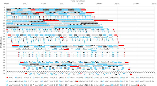
6.2. Validation

The validation of the obtained schedules is done by checking the Gantt charts for the 12 runs (12 days). Three jobs are selected (Job no. 1, 26 and 50) for two days (Day no. 2 and 8) where their routes are traced to check that they are treated at the right stages and within the right durations according to their recipe. In-addition, the treatments’ durations of the same jobs are checked to make sure they are not overlapping. Same check-up is done for the remaining jobs (i.e. all the jobs), to ensure that the simulations are valid. The Gantt charts of the two selected days are included in Appendix A.

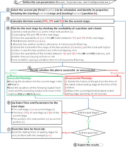
6.3. Evaluation

The evaluation is conducted to show the algorithm strength in minimizing the anodizing makespan. For every job produced during the selected twelve days, the actual and simulated anodizing finishing times are compared. It is found that for most of the jobs, the algorithm is able to finish them before the actual finishing time, except for some jobs that are usually processed at the beginning of the day. Plots of these times with their differences can be seen for Days no. 2 and 8 in Figures 2 and 3.

Figure 2. Day no. 2 job flow time at the anodizing stage evaluation chart.

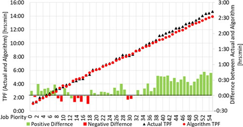
Figure 3. Day no. 8 job flow time at the anodizing stage evaluation chart.

As for the last jobs, the differences between the actual anodizing finishing times and the algorithm anodizing finishing times are positive, as shown in Table 3. This means the algorithm succeeded in reducing the anodizing makespan, where the average difference between the actual and the algorithm makespans is found to be 2:42:10 (hrs:min:sec), i.e. 18% reduction from the actual makespan. The highest difference is 4:15:19 (26.76%), while the lowest is 00:43:41 (4.97%), both are shown in shaded cells in Table 3. However, these large reductions may be due to the occurrence of the implicit breakdowns in the actual production.

6.4. Stages utilization percentages and bottleneck identification

The total of the daily treatment durations of each position is divided by the makespan of that day to get the daily utilization percentage of each position. Then, the utilization percentages of the positions that belong to one stage are averaged out to get the daily utilization percentage of each stage (SU (%)). The results shown in Table 4 reveal that the Hot Sealing, Anodizing and Etching stages are the chemical stages with the highest daily average utilization percentages of 61%, 44% and 35%, respectively. Since none of them is 100% or near 100%, the results do not identify a presence of a bottleneck among the chemical stages. Although the results show a higher utilization percentage for the Input Buffer Zone 2 of 75%, it cannot be considered a bottleneck even if it reaches 100%, because it is a waiting stage.

Table 4. The daily average percentage of utilization of each stage.

Stage name	SU (%)	Stage name	SU (%)
Input Buffers Zone 2	74.93	Electro-Coloring	7.39
Loading	61.47	Transferor 2	5.91
Hot Sealing	61.38	Demi-Rinsing	5.91
Input Buffers Zone 1	59.89	Desmutting	4.13
Anodizing	43.53	Anodizing Rinsing	3.91
Etching	34.80	Electro-Coloring Rinsing	2.16
Un-Loading	23.33	Desmutting Rinsing	2.07
Alkaline	18.63	Alkaline Rinsing	2.05
Etching Rinsing	18.16	Output Buffers Zone	1.70
Transferor 1	14.11

7. Experimentation and analysis of results

7.1. Effect of combinations on makespan

The first objective of the experimentations is to study the combinations effect on reducing the makespan. Table 5 shows the makespans for all the nine combinations for the twelve days, and counts the score for each combination when it has the minimum makespan among the other combinations. It can be seen from the table that the best combination is S3C2 with 50% likelihood to score the minimum makespan, where it has obtained the minimum makespan in six days.

Table 5. Effect of different combinations on the makespan and added number of jobs.

Day	Effect of combinations on the makespan										Effect after adding jobs
											S1C1		SXC1
	Makespan by the algorithm (hrs:min:sec) per combination									Minimum makespan	Added jobs (%)	Time utilized (%)	SX	Added jobs (%)	Time utilized (%)
	S1C1	S1C2	S1C3	S2C1	S2C2	S2C3	S3C1	S3C2	S3C3
1	14:33:41	14:03:29	14:03:29	15:08:09	13:02:10	13:02:10	13:45:07	13:02:12	12:54:23	S3C3	9.43	98.77	S3	16.98	99.03
2	15:03:04	14:46:37	15:03:28	15:22:30	14:51:10	15:16:28	14:54:56	14:36:10	15:22:39	S3C2	5.45	99.33	S3	7.27	99.21
3	14:40:29	14:08:40	14:08:40	14:29:11	15:08:50	14:53:10	14:40:09	14:38:59	14:40:46	S1C2 & S1C3	12.50	99.87	S2	18.75	99.90
4	13:02:40	12:38:54	12:28:41	12:17:39	12:21:30	12:21:50	13:00:46	12:56:47	12:56:47	S2C1	26.09	95.92	S2	28.26	99.33
5	12:57:31	12:42:50	12:51:10	14:26:58	14:26:58	15:15:22	12:29:41	11:56:05	11:56:05	S3C2 & S3C3	26.09	95.51	S3	32.61	97.16
6	14:19:06	14:24:11	14:17:31	13:30:48	14:02:00	14:02:20	13:15:21	12:58:04	12:58:24	S3C2	19.57	99.43	S3	19.57	98.08
7	12:44:01	12:55:12	12:04:48	12:43:31	12:44:11	12:44:11	13:07:55	11:43:07	12:45:54	S3C2	31.11	96.08	S2	28.89	96.73
8	13:33:27	13:05:49	13:03:09	12:55:48	12:16:44	12:17:04	13:10:40	11:55:04	11:48:26	S3C3	14.00	94.60	S2	24.00	96.13
9	13:09:10	12:36:32	12:36:40	12:51:17	11:57:28	12:11:58	13:03:40	12:16:15	12:11:39	S2C2	25.53	98.27	S2	29.79	96.49
10	13:36:32	12:31:32	12:16:01	13:25:57	14:10:00	14:10:41	14:05:29	12:14:45	12:15:25	S3C2	18.37	97.89	S2	18.37	96.29
11	14:05:33	13:15:16	13:51:57	14:33:23	14:20:45	14:20:45	13:25:05	13:35:12	12:56:59	S3C3	17.31	98.85	S3	17.37	98.23
12	13:52:06	13:17:06	13:18:48	14:17:01	12:43:59	12:44:19	13:35:15	12:35:07	13:38:05	S3C2	20.00	97.05	S3	18.00	95.28
Score	0	1 (0 + 1)	1 (0 + 1)	1 (1 + 0)	1 (1 + 0)	0	0	6 (5 + 1)^a	4 (3 + 1)	Average	18.79	97.63	–	21.66	97.66

^a Minimum makespan of one day out of 6 days results is obtained also by another combination.

7.2. Effect of combinations on improving the performance of the Hot Sealing and Anodizing stages

The second objective of the experimentation phase is to examine the effect of the nine combinations on improving the performance of the Hot Sealing stage and the Anodizing stage. To study this, the roundup daily average number of jobs that are treated in the anodizing tanks and the hot sealing tanks are used. In Table 6, the shaded positions are the actual ones in the plant, while non-shaded are additional position(s) replacing other position(s) as mentioned in Sub-section 3.4 point (b). As it can be seen in Table 6, the results suggest to add one more hot sealing tank (position 47) and no additional anodizing tank is needed (position 36 not needed), because it is not used. As for the second additional hot sealing tank (position 48), the roundup average number of jobs is increased by only one job, thus this additional hot sealing tank is not needed either. Because, it is noticed that with configuration 2, which has only one additional hot sealing tank, 52 jobs are treated, while with configuration 3, which has two additional hot sealing tanks, 51 jobs are treated. Thus, configuration 2 is achieving higher output than configuration 3 if not the same. In Table 6, the total numbers of jobs for the different combinations in the Anodizing and the Hot Sealing tanks are not the same, due to the different number of positions in each combination, and different for the same combination due to the round-up number of jobs. Roundup is done to deal with the number of jobs as an integer number.

Table 6. Average number of jobs (Round-up) in anodizing and hot sealing tanks for the nine combinations.

Stage	Position No.	Average number of jobs per combination
		S1C1	S1C2	S1C3	S2C1	S2C2	S2C3	S3C1	S3C2	S3C3
Anodizing	30	15	19	19	19	19	19	19	19	19
	31	13	17	17	17	17	17	17	16	16
	33	12	12	12	12	11	11	12	13	12
	34	10	3	3	3	3	3	3	3	3
	36	–	0	0	–	0	0	–	0	0
Hot Sealing	43	22	20	20	22	21	21	22	21	21
	44	10	10	10	11	11	11	11	10	10
	45	10	9	9	10	10	10	10	9	9
	46	8	8	8	8	7	7	9	8	7
	47	–	4	4	–	3	3	–	4	3
	48	–	–	1	–	–	0	–	–	1
Anodizing Total Jobs		50	51	51	51	50	50	51	51	50
Hot Sealing Total Jobs		50	51	52	51	52	52	52	52	51

7.3. Further experimentations

The aim of this experimentation phase is to increase the number of jobs produced in an attempt to fully utilize the remaining time left out from the day time (16 hours) after minimizing the makespan. These experimentations are concerned with the actual plant, where the number of combinations is narrowed down to only two combinations. The two combinations considered are for the actual configuration (Configuration 1), but one with the actual sequence (Sequence 1) named the “actual combination” (S1C1), while the other with the sequence that produced the minimum makespan named the “minimum combination” and designated SXC1 The designation SXC1 means to compare the combinations (S1C1, S2C1, and S3C1), where the minimum makespan among these three combinations is in bold font in Table 5. In this analysis, the jobs are added one by one through a loop consisting of two types of jobs, the loop starts with two jobs of recipe no. 3 (Matt Finish profiles), and then one job of recipe no. 6 (Colored Finish profiles), and then returns to add two jobs of recipe no. 3 and so on. The loop stops whenever the finishing time of one of the jobs at the unloading stage exceeds the day time (16 hours), thus this last job is excluded, while the other jobs are taken. Recipe no. 3 and 6 are chosen, because they are the most commonly produced types of profiles and they add a variety to the loop.

The results show that the two combinations are quite the same in term of the number of added jobs and in term of the percentage of full day time utilization. Where the average percentages of added jobs are 18.79% and 21.83% for the two combinations, namely actual combination and minimum combination, respectively, while average time utilization percentages are 97.63% and 97.60% for the two combinations, respectively. The results for all days are shown in Table 5.

8. Conclusion

In this work, a real anodizing plant is modelled to re-schedule the production of twelve days in an attempt to reduce the actual makespan for each day, and to increase the production.

A mathematical model is proposed that describes the detailed movements in the system, yet this mathematical model is not fully translated in the programmed algorithm, due to its complexity. An algorithmic solution approach is adopted, and it is programmed using Matlab R2015b editor. The algorithm computational time is 2.5 min for each run. The runs of the simulation are divided into three phases, where each phase has its own objectives.

The developed heuristic algorithm reduces the anodizing makespan by an average of 18% for the first combination (the currently used combination). In addition, the results of the nine combinations tested by the simulation model show that re-designing the plant by adding one additional hot sealing tank and prioritizing the jobs based on the third sequence (Highest Recipe ID First) forms the best combination to reduce the makespan and to improve the performance of the Hot Sealing stage. The average increase in the number of jobs of highly demanded recipes that the algorithm can achieve is around 20%, which results into an average time utilization of 98%.

The proposed algorithm can be used by the planning department in the concerned company to determine the best sequence of jobs for the production of any day consisting of two shifts by giving the list of the prioritized jobs including the jobs recipes. The study also suggests adding one additional Hot Sealing tank to improve the production of this stage.

Further research to be undertaken is to improve the algorithm by removing the relaxations mentioned in Sub-section 3.2. In-addition, more experimentations may be conducted such as adding extra tanks to the Etching stage to improve the performance of this stage and to study the effect of changing the hoists’ ranges on the makespan.

Acknowledgements

The authors are thankful to the former CEO of the concerned company for giving the opportunity to conduct this research; the authors are also thankful to the production manager and to the workers who provided the necessary information needed to complete this work.

This work is extracted from a thesis submitted in partial fulfillment for M.Sc. degree in Engineering Management offered by the University of Bahrain.

Disclosure statement

No potential conflict of interest was reported by the authors.

Appendix A:

Gantt charts for Day no. 2 and Day no. 8 (Combination 1)

Figure A.1. Gantt chart for Day no. 2 with Combination 1.

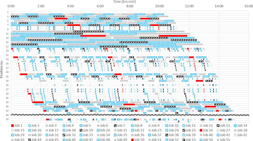
Figure A.2. Gantt chart for Day no. 8 with Combination 1.

References

- Basán, N. P., Pulido, R., Cóccola, M. E., & Méndez, C. A. (2017). Aerospace manufacturing industry: A simulation-based decision support framework for the scheduling of complex hoist lines. Iberoamerican Journal of Industrial Engineering, 9(17), 100–117.
- Bloch, C., Manier, M. A., Baptiste, P., & Varnier, C. (2010). Hoist scheduling problem. Production Scheduling, 193–231.
- Che, A., Kats, V., & Levner, E. (2017). An efficient bicriteria algorithm for stable robotic flow shop scheduling. European Journal of Operational Research, 260(3), 964–971. doi:10.1016/j.ejor.2017.01.033
- El Amraoui, A., Manier, M. A., El Moudni, A., & Benrejeb, M. (2013). A genetic algorithm approach for a single hoist scheduling problem with time windows constraints. Engineering Applications of Artificial Intelligence, 26(7), 1761–1771. doi:10.1016/j.engappai.2013.02.004
- Elmi, A., & Topaloglu, S. (2013). A scheduling problem in blocking hybrid flow shop robotic cells with multiple robots. Computers & Operations Research, 40(10), 2543–2555. doi:10.1016/j.cor.2013.01.024
- Elmi, A., & Topaloglu, S. (2017). Multi-degree cyclic flow shop robotic cell scheduling problem with multiple robots. International Journal of Computer Integrated Manufacturing, 30(8), 805–821. doi:10.1080/0951192X.2016.1210231
- Feng, J., Che, A., & Chu, C. (2015). Dynamic hoist scheduling problem with multi-capacity reentrant machines: A mixed integer programming approach. Computers & Industrial Engineering, 87, 611–620. doi:10.1016/j.cie.2015.06.004
- Lei, W., Manier, H., Manier, M. A., & Wang, X. (2017). A hybrid quantum evolutionary algorithm with improved decoding scheme for a robotic flow shop scheduling problem. Mathematical Problems in Engineering, 2017, 1–13. doi:10.1155/2017/3064724
- Liu, C., Zhao, C., & Xu, Q. (2012). Integration of electroplating process design and operation for simultaneous productivity maximization, energy saving, and freshwater minimization. Chemical Engineering Science, 68(1), 202–214. doi:10.1016/j.ces.2011.09.024
- Mateo Doll, M., Manier, M. A., & Companys Pascual, R. (2015). A procedure based on branch-and-bound for the Cyclic Hoist Scheduling Problem with n types of product. A: International Conference on Industrial Engineering and Industrial Management. International Conference on Industrial Engineering and Operations Management. International IIE Conference. “Engineering Systems and Networks: the way ahead for industrial engineering and operations management”. Aveiro: 2015, p. 1–8.
- Pantusavase, K., & Hassamontr, J. (2015). Enumerative search for crane schedule in anodizing operations. World Academy of Science, Engineering and Technology, International Journal of Mechanical. Aerospace, Industrial, Mechatronic and Manufacturing Engineering, 9(6), 1052–1058.
- Paul, H. J., Bierwirth, C., & Kopfer, H. (2007). A heuristic scheduling procedure for multi-item hoist production lines. International Journal of Production Economics, 105(1), 54–69. doi:10.1016/j.ijpe.2005.11.008
- Skov, J. (2007). Scheduling of an Anodizing Plant at Bang & Olufsen (Unpublished master thesis). University of Southern Denmark, Odense, Denmark.