What Should We Do Differently in STAT 101?

Abstract

The introductory statistics course has gotten better over the years, but there are many content areas in STAT 101 that should be reconsidered.

KEYWORDS:

• Berkson
• Causal diagram
• Cornfield
• Effect size
• Significance
• Simpson

STAT 101 is a much better course today than it was when I started teaching (many years ago). We use real data. We teach randomization-based inference. We have students do projects, so that they experience the entire cycle of statistical work. We use computer simulation. We use activities. I could go on.

There is a lot one could write about pedagogy (“How”) but my interest here is on topics and course content (“What”). The statistics education community has added many topics to STAT 101 over the years and let go of others, but there is more to be done. In this article I’ll discuss 15 changes I would like to see in the introductory course.

I must acknowledge up front that there are textbooks that include some of these 15 ideas and that most, if not all, statistics educators already do at least some of the things I am about to suggest. But as I look at popular textbooks or the AP Statistics syllabus—which is designed to reflect the typical STAT 101 course—I see a course that could be improved. The GAISE College report provides valuable guidance, but more on a global level about pedagogy than on directing us to teach specific topics.

I also acknowledge, as does the GAISE College report, that there are many flavors of introductory statistics. I’m thinking about a course for a general audience that presents statistical thinking (data collection and representation) along with inference (tests and intervals) and a bit of modeling (regression). Some topics on my list are more important or less important depending on the particular students in the course. Moreover, the philosophy of statistics education that motivates me here is that I want students to develop data acumen and an orientation toward modeling and prediction, putting somewhat less emphasis on formal statistical inference and on learning a list of inference methods that are widely used. When I review requests for transfer credit for introductory statistics I can check whether the course in question covers a certain set of methods (t-test, Chi-square test, paired data, etc.) because that is what I can glean from a course catalog description, but what I care more about is whether the course promotes statistical reasoning, modeling, and prediction. Sadly, I cannot assume that it does.

In what follows I will divide my recommendations into three categories. The first category contains changes that could be implement quickly. That is, while walking from your office to your classroom you could decide to make one of these changes and then implement that change a few minutes later. The second category contains changes to a course that you could implement after investing a day or so of planning. The third category includes changes to a course that would require more planning, but that are worth considering, nonetheless.

Category (a): Changes You Could Make with Little Effort or Planning.

• Change 1: We use the words “statistically significant” and thus confuse students, readers, and ourselves. For example, here is a quote from a Ph.D. statistician: “Since this p-value is less than 0.05, that means that H ${}_0$ is rejected and there is a significant difference in degree completion status between men and women.” I’m sure that I’ve said similar things in the past, but the statement is not correct. What we should say is that there is evidence of a difference between men and women. The word “significant” gets in the way of clear thinking here.

The word “significant” is so widely used outside of statistics that many users of statistics seem to think that “statistically significant” means “important,” not realizing that having a small p-value only means that the sample size was large enough that we can be confident that sampling variability wasn’t the cause of the observed effect. Rather than calling a result “statistically significant” we could call it “statistically discernible” (Witmer 2019), as at least some authors have started to do (Chihara and Hesterberg 2022).

• Change 2: We report p-values to too many digits. My computer can tell me that with a t-statistic of 1.31 on 12 degrees of freedom the two-tailed p-value is 0.214719, but most of those digits are meaningless. Yet our students, having taking many mathematics classes, like to report as many digits as they can. Let’s tell them “P $=$ 0.2” and disabuse them of the notion that the other digits matter. We are teaching statistics, not mathematics. In mathematics 0.3 is not the same as 0.33 which is not the same as 1/3, but I’ve never seen a statistical analysis in which P $=$0.3 versus P $=$0.33 mattered. Yet reporting the p-value to many digits gives the student the idea that those digits are important and believable, as if they were studying mathematics, while their attention really should be on other matters.

If the p-value is less than 0.1, then a second or third decimal can be useful; that is, someone might care that P $=$0.008 is different from P $=$0.014, but they should not care about P $=$0.0077 versus P $=$0.0082.

• Change 3: Some people still talk about assumptions rather than about conditions. But the word “assumptions” implies that we can, and should, assume something. Mathematicians love to start with assumptions and then reason to a conclusion and they often don’t care whether the assumptions bear any relationship to the real world. But statistics is different: If our conditions are not satisfied, then we can still fit a model but we cannot trust the accuracy of a p-value or confidence interval that software might give us. Sometimes we have to make an assumption about part of the statistical process, but often we can check a condition, such as normality of the underlying population.

• Change 4: Many books use X as the generic random variable early in the book but then use Y for the response variable when discussing regression. Some use X in the ANOVA chapter. There is no good reason for this inconsistency that suggests to the student that regression modeling is an entirely different activity than conducting a t-test, say. Let’s call the (response) variable Y for the entire course, starting in the first chapter the textbook, both to minimize cognitive load for the student and to promote modeling and prediction throughout the course.

Of course, if you have adopted a textbook that uses X for the first several chapters of the book then you probably will want to use that same notation when teaching—so the thing you might decide to do while walking from your office to your classroom is to mentally compose a letter to the author of the textbook.

Category (B): Changes to a Course That You Could Implement after Investing a Day or so of Planning.

• Change 5: Rightly or wrongly, statisticians are seen as greatly overselling hypothesis testing and this is due in no small part to the fact that most STAT 101 courses spend a lot of time on inference, primarily testing. Students develop the idea that p-values are good, consistent measures of strength of evidence, but they are not (Wasserstein, Schirm, and Lazar 2019). (See The Dance of the p-Values.¹) Moreover, a hypothesis test only answers one very specific and narrow question: How likely is it that data such as these would arise by chance. At times that can be a very important question, but not always. (I’ll resist the temptation to write several pages on the difference between what a hypothesis test addresses and what people usually want to know; namely, How likely is it that the null hypothesis is true, given these data?) Let’s use more modeling and estimation and less formal inference.

• Change 6: We stress Type I errors but not power and Type II errors. We know that Type II errors can be very important; for example, when it comes to COVID-19 vaccine development it is Type II error that matters. Yet we spend the lion’s share of time looking at p-values and worrying about Type I errors, asking questions such as “What α did you use?” but rarely asking “How much power did the test have?” It matters that many studies are underpowered (van Zwet, Schwab, and Greenland 2021) and statisticians know that “Absence of evidence is not evidence of absence” but textbooks don’t say much about power, perhaps because it is difficult to present mathematically.

However, we can teach power with computer simulation, so let’s do that. For example, Allan Rossman has a nice pair of blog posts about power simulation in the context of a basketball player shooting free throws, which students find easy to understand and to implement.² When completing this activity they see that as the sample size changes, the chance of detecting an effect changes. Likewise, they see that as the size of an effect grows we can detect the effect more easily.

• Change 7: We teach about p ${}_1$–p ${}_2$ but not about p ${}_1$/p ${}_2$ when often relative risk is what people care about; for example, you are not likely to get lung cancer even if you smoke, but being a smoker increases the risk of lung cancer 10-fold over being a nonsmoker (Hansen et al. 2020) and it is that increased risk that matters. Conducting inference for relative risk, or for an odds ratio, is complicated (although it is presented in some introductory books; see Chance and Rossman 2022), but we can and should at least show students the topic of relative risk.

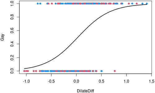
• Change 8: Most introductory textbooks don’t present logistic regression, although there are exceptions (see Cetinkaya-Rundel and Hardin 2021). But given that we are using software to fit the models, doing logistic regression is not much more difficult than doing ordinary least-squares regression. Let’s at least expose our students to this powerful tool in STAT 101. If you use R with your students, then you can tell them to change “lm(y $\sim$ x, data $=$ mydata)” to “glm(y $\sim$ x, family $=$ binomial, data $=$ mydata)” and let the computer do the rest. Of course, the logistic model is linear in log(odds) and it is a lot more complicated to say “As x increases by one unit, the odds of success are multiplied by 1.3” than it is to say “As x increases by one unit, y increases by 1.3 units;” but we can still show logistic curves to students and let them know that there is a sensible way to model the relationship between a quantitative predictor and a dichotomous response. Students are going to see logistic regression used more and more often so they should have some understanding of what it is—even if developing deep understanding needs to wait until the second course.

As an example, I show my students the graph in Figure 1, which is derived from data in the article “The Eyes Have It” (Rieger and Savin-Williams 2012) in which researchers use pupil dilation difference as a predictor of sexual orientation. Here the response is coded as 1 for subjects who are gay and 0 for subjects who are straight. These subjects have looked at images of nude females and of nude males while a device measured the dilation of their pupils, which is a nonvoluntary response to visual stimulus. The predictor is the difference in pupil dilation for same-sex nudes minus opposite sex nudes, so a positive DilateDiff means that pupil dilation was greater when gazing at same-sex nudes. This measurement is strongly associated with sexual orientation. Students get the idea immediately and they find the example to be stimulating, if I may use that word.³

Fig. 1 Logistic curve modeling the relationship between pupil dilation and sexual orientation. Points are colored by sex of the subjects (blue for male and red for female).

• Change 9: We tell students that there are standard methods to deal with each of these settings: 1 mean, 2 means, paired means, 1 proportion, and 2 proportions. Let’s at least mention that there is a test for paired proportions. You might not want to take valuable class time to teach your students how to conduct McNemar’s test, but it only takes a minute or two to tell students that it exists.

If you do want to teach the analysis of paired proportion data, here is an example. A few years ago the Atheist shoes company, in Germany, was worried that too many of their shipments to the U.S. were getting “lost” in the mail, so they ran an experiment in which they sent pairs of packages to 89 U.S. addresses.⁴ Each pair included one package sealed with Atheist-branded packing tape and one package sealed with neutral tape. For 79 addresses both packages arrived, but there were 10 for which only one package arrived. If the type of packing tape makes no difference then we would expect the 10 “discordant” pairs to split evenly, with the Atheist package to be the one that was lost five times; but the actual count was 9, not 5. Is a 9 – 1 split more imbalanced than would be expected by chance? These are paired proportion data and McNemar’s test is the tool we need.⁵

Category (C): Changes to a Course That Would Require Quite a Bit of Planning but That Are Worth Considering Nonetheless

• Change 10: We should talk about effect size. We tell students to find a p-value and then reject or retain H ${}_0$, but sometimes the effect is so modest that we shouldn’t expect anyone to care about it, yet we had such a large sample size that we had enough power to reject the null. To take one example, heavy smokers were compared to moderate smokers on lung function (White and Froeb 1980). For moderate smokers the mean forced mid-expiratory flow, in liters/sec, was 2.73 with an SD of 0.81, while heavy smokers were lower at 2.59 with an SD of 0.82. Applying a hypothesis test gives a p-value of 0.04, something most would call “statistically significant” (or just “significant,” which is wording that I have critiqued above) and yet the effect size is only 0.17, so moderate smokers do better than heavy smokers by only about 1/6 of a standard deviation.

As teachers we know that p-values go down as sample sizes increase and we tell this to our students, but we should be more direct and tell them test stat $=$ (effect size)*(sample size inflation)

For example, for a t-test, $$t=\frac{\overline{y}-\mu }{s}\ast \sqrt{n}$$

For example, for a two-sample t-test, $$t=\frac{{\overline{y}}_1-{\overline{y}}_2}{s}\ast \sqrt{\frac{n_1{n}_2}{n_1+n_2}}$$

For example, for a correlation t-test (equivalent to a slope t-test), $$t=\frac{r}{\sqrt{1-r^2}}\sqrt{n-2}$$

For example, for an F-test, $$\begin{array}{c}F=\frac{R^2}{1-R^2}\left(n-2\right)\hspace{1em}\text{or}\\ F=\frac{S{S}_m}{S{S}_r-S{S}_m}\left(n-2\right)\hspace{1em}\text{or}\\ F=\frac{S{S}_m}{\mathit{SSE}(n-2)}\end{array}$$where r stands for “response” and m stands for “model.”

More generally, this is $F=\frac{R^2}{1-R^2}\frac{(n-(k+1))}{k}$.

It might be a bit much to add discussion of effect size to every inference topic in a course, but at a minimum students studying the two-sample mean situation should think about the difference in sample means, scaled by the standard deviation. Of course, the two sample SDs won’t be the same, but I tell my students that they can just use the larger of the two SDs—and that if the two SDs are wildly different, then we should question a comparison of means in the first place.

• Change 11: We warn students about the multiple testing problem (see https://xkcd.com/882/) but not about the garden of forking paths (see https://xkcd.com/1478/ and Gelman and Loken 2014). We tell our students that we should not start with a nondirectional alternative hypothesis, see in which direction the data point, and then do a test using that directional alternative; it is easy to see how such a practice would result in an invalid p-value that is half the size of the nondirectional p-value. The garden of forking paths idea is similar, but more subtle. The main idea is that there is often more than one hypothesis we could test and we could sift through the data until we find a pair of subgroups that differ. We might fool ourselves, or others, and only conduct one formal hypothesis test while telling ourselves that there is no need to adjust for multiple testing since we only conducted one (formal) test. But along the way we might have made a series of decisions (“Should I keep this outlier?” “Does it really make sense to include subjects for whom English is a second language?” etc.) that lead us to a comparison that yields a small p-value, while informally conducting other tests.

On a related note, let’s tell our students more about publication bias. For example, a study of FDA trials of antidepressants (Turner et al. 2008) found that 37 of 38 positive results were published but only 3 of 36 negative results were published, which means that over 90% of the published results had evidence of antidepressants working despite them working in only about half of all clinical trials.

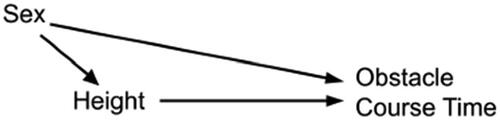
• Change 12: We tell students that causal inference is only allowed following a randomized experiment. This is like telling them that sex is only allowed within a marriage: No matter how often the message is repeated, we can’t change human nature. Instead, let’s present causal diagrams and think about how to deal with confounding (Cummiskey et al. 2020). For example, I do an activity in my introductory class that takes up one class session. We look at a scatterplot of time versus height for cadets at West Point completing the Indoor Obstacle Course Test. Tall cadets tend to have better times, but the confounding variable Sex is responsible for this. The relevant causal diagram is shown in Figure 2. Multiple regression could be used here, but I just have my students split the data by Sex and then do a simple regression with each subgroup, showing that Height doesn’t really matter within Sex categories.

Fig. 2 Causal diagram for the relationships among Sex, Height, and Time to complete the Indoor Obstacle Course Test at West Point.

Materials for this activity can be found at https://github.com/kfcaby/causalLab.

Causal diagrams are not part of the STAT 101 textbook world and introducing even a short unit on causal reasoning with observational data means needing to cut out something else, such as any discussion of probability, but the tradeoff is worth it. There may be a time or two in a student’s life when facility with formal probability will be useful, but there will be countless times when being able to reason about causation will be useful.

• Change 13: We teach prediction intervals only in the regression chapter. Why not get students thinking about statistical prediction by saying more about it in the 1-sample chapter? If we decide that a drug works let’s go beyond saying by how much, with a CI for µ, and let’s also make a prediction for one person’s response, with a PI. One step in this direction is to remind students that if we have a reasonably bell-shaped histogram then the mean ± 2*SD covers 95% of the data, so if we want to give an interval that has a high chance of including an individual point we can look at the mean ± 2*SD, whereas the 95% CI – mean ± 2*SE – does not contain 95% of the data. Statisticians build models to understand the world but also to make predictions (albeit usually in a multivariate setting). Let’s put more of the spirit of prediction into our courses and not confine prediction to the regression chapter.

• Change 14: We teach Simpson’s paradox;⁶ let’s also be explicit about how to adjust for a confounder. There are many examples of Simpson’s paradox, one of which comes from the state of Florida where White defendants in assault cases who invoked the “stand your ground” defense were more likely to be convicted than were Black defendants, overall. But if we condition on the race of the victim then this relationship reverses, with Black defendants more likely to be convicted if the victim in Black or if the victim is White (Witmer 2015). Figure 3 is a causal diagram for this situation.⁷

Fig. 3 Causal diagram for the relationships among the race of the victim, the race of the defendant, and whether or not the defendant was convicted.

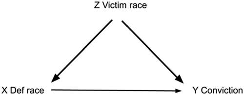
To adjust for the confounder of victim’s race, we could ask “What would the conviction rate be of White or of Black defendants if their victims had the same racial distribution (e.g., 60% White and 40% Black)?”

Another way to think about the effect of a confounder is to split the data on the confounder and do an analysis of each subset, as mentioned with item #12 above.

Related to this, let’s teach the Cornfield conditions. In this example the Cornfield conditions tell us that the association between X and Y will only be reversed if the arrows from Z to X and from Z to Y are both thicker than the arrow from X to Y; that is, that the association between Z and X and the association between Z and Y are both stronger than the association between X and Y (see Cornfield et al. 1959; Ding and Vanderweel 2014).

• Change 15: Let’s teach Berkson’s paradox. For example, there is a negative association between pitching ability and hitting ability among major league baseball players. The thing is, most of us can’t pitch and we can’t hit, so we are not in the major leagues. To get into the major leagues you have to be very good at one of those two things (or both, in very rare cases) so when we look at just MLB players we see a negative association that is not present in general.

As another example, early during the pandemic doctors were surprised to notice a negative association between COVID-19 and smoking among patients in hospitals, as if smoking were somehow a preventative.⁸ But the words in italics are important because restricting attention to those in hospitals induces a negative association between health problems. The appropriate causal diagram, Figure 4, shows a collider.

Fig. 4 Causal diagram (a collider) for the relationships among smoking status, COVID-19 status, and hospitalization.

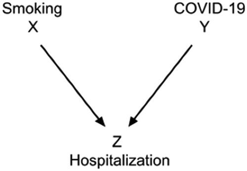
If you aren’t a smoker, then you are more likely to have COVID-19, because you are in the hospital due to some illness (i.e., hospitalized patients are not representative of the general population).⁹

I could name other changes to STAT 101 content, as could you, and many of you are already doing some of the 15 things I’ve mentioned. I hope that textbook authors will make it easier for more educators to include topics that students really should see.

You might like one or more of these suggestions but wonder how you could possibly add more to an already overcrowded course. Given that the STAT 101 course I have in mind is probably required for students in multiple majors, it is not easy to reduce coverage of topics that faculty in other departments want their majors to learn. I have two specific suggestions. First, consider eliminating probability. Most introductory courses teach less probability today than in the past, but the AP Statistics curriculum still has probability as one of four “skill categories” and the AP Statistics exam gives 10%–20% weight to probability, random variables, and probability distributions. I suggest 0%–5% weight, with 0% being a viable option.

Second, STAT 101 often includes basic work with descriptive statistics and graphs (i.e., histograms, dotplots, and boxplots). But most U.S. high school graduates have already been taught this material because their state has either adopted the Common Core or something similar. Introductory textbooks continue to include this basic material, but college faculty don’t need to spend class time on this and can instead devote more time to helping students develop statistical reasoning skill, with an orientation toward modeling, understanding relationships, and making predictions.

Acknowledgments

Some of the ideas above were inspired by conversations with Kevin Cummiskey, Danny Kaplan, Milo Schield, and others. None of them approved of me taking their ideas and using them in this article; not that I asked. I also thank the reviewers of an earlier version of this work whose advice led me to substantially change the article.

Data Availability Statement

Data sharing is not applicable to this article as no new data were created or analyzed in this study.

Disclosure Statement

The author reports that there are no competing interests to declare.

Notes

1 https://www.youtube.com/watch?v = 5OL1RqHrZQ8

2 See https://askgoodquestions.blog/2021/01/11/80-power-part-1/ and https://askgoodquestions.blog/2021/01/18/81-power-part-2/; also there is a third post about power that is more mathematical than these two.

3 I also show students a graph with parallel logistic curves for male and female subjects and discuss how the gap between the curves relates to bisexuality being more common among females than males.

4 See https://atheist.shoes/pages/usps-study.

5 Pr(Y = 9 or 10 out of 10 | $p = 0.5$) = 0.0098 + 0.0009 ≈ 0.01.

6 There is a rich collection of papers about teaching Simpson’s paradox available at https://www.tandfonline.com/journals/ujse20/collections/teaching-simpsons-paradox

7 We might think that the arrow should point from X to Z. However, on page 312 of their book, Pearl and Mackenzie (2018) discuss the direct effect of X on Y, in contrast to the total effect. If we care about the direct effect that the race of the defendant has on conviction then Figure 3 is the appropriate causal diagram.

8 https://www.qeios.com/read/WPP19W.3

9 https://rss.onlinelibrary.wiley.com/doi/10.1111/1740-9713.01413 and https://www.newscientist.com/article/2243944-smoking-probably-puts-you-at-greater-risk-of-coronavirus-not-less/

References

- Cetinkaya-Rundel, M., and Hardin, J. (2021), “Introduction to Modern Statistics,” OpenIntro, available at https://leanpub.com/imstat.
- Chance, B., and Rossman, A. (2022), Investigating Statistical Concepts, Applications, and Methods (4th ed.), available at http://www.rossmanchance.com/iscam3/.
- Chihara, L., and Hesterberg, T. (2022), Mathematical Statistics with Resampling and R (3rd ed.), New York: Wiley.
- Cornfield, J., Haenszel, W., Hammond, E. C., Lilienfeld, A. M., Shimkin, M. B., and Wynder, E. L. (1959), “Smoking and Lung Cancer: Recent Evidence and a Discussion of Some Questions,” Journal of the National Cancer Institute, 22, 173–203.
- Cummiskey, K., Adams, B., Pleuss, J., Turner, D., Clark, N., and Watts, K. (2020), “Causal Inference in Introductory Statistics Courses,” Journal of Statistics Education, 28, 2–8. DOI: 10.1080/10691898.2020.1713936.
- Ding, P., and Vanderweel, T. J. (2014), “Generalized Cornfield Conditions for the Risk Difference,” Biometrika, 101, 971–977. DOI: 10.1093/biomet/asu030.
- GAISE College Report ASA Revision Committee, “Guidelines for Assessment and Instruction in Statistics Education College Report 2016,” available at http://www.amstat.org/education/gaise.
- Gelman, A., and Loken, E. (2014), “The Statistical Crisis in Science,” American Scientist, 102, 460–465. DOI: 10.1511/2014.111.460.
- Hansen, M. S., Licaj, I., Braaten, T., Lund, E., and Gram, I. T. (2020), “The Fraction of Lung Cancer Attributable to Smoking in the Norwegian Woman and Cancer (NOWAC) Study,” British Journal of Cancer, 124, 658–662. DOI: 10.1038/s41416-020-01131-w.
- Pearl, J., and Mackenzie, D. (2018), The Book of Why: The New Science of Cause and Effect, New York, NY: Basic Books.
- Rieger, C., and Savin-Williams, R. C. (2012), “The Eyes Have It: Sex and Sexual Orientation Differences in Pupil Dilation Patterns,” PLoS One, 7, e40256. DOI: 10.1371/journal.pone.0040256.
- Turner, E. H., Matthews, A. M., Linardatos, E., Tell, R. A., and Rosenthal, R. (2008), “Selective Publication of Antidepressant Trials and its Influence on Apparent Efficacy,” The New England Journal of Medicine, 358, 252–260. DOI: 10.1056/NEJMsa065779.
- van Zwet, E., Schwab, S., and Greenland, S. (2021), “Addressing Exaggeration of Effects from Single RCTs,” Significance, 18, 16–21. DOI: 10.1111/1740-9713.01587.
- Wasserstein, R. L., Schirm, A. L., and Lazar, N. A. (2019), “Moving to a World Beyond ‘p < 0.05’,” The American Statistician, 73, 1–19. DOI: 10.1080/00031305.2019.1583913.
- White, J. R., and Froeb, H. F. (1980), “Small-Airways Dysfunction in Nonsmokers Chronically Exposed to Tobacco Smoke,” The New England Journal of Medicine, 302, 720–723. DOI: 10.1056/NEJM198003273021304.
- Witmer, J. (2015), “How Much Do Minority Lives Matter,” Journal of Statistics Education, 23, 1–9. DOI: 10.1080/10691898.2015.11889739.
- Witmer, J. (2019), “Editorial,” Journal of Statistics Education, 27, 136–137. DOI: 10.1080/10691898.2019.1702415.