Causal Inference Is Not Just a Statistics Problem

Abstract

This article introduces a collection of four datasets, similar to Anscombe’s quartet, that aim to highlight the challenges involved when estimating causal effects. Each of the four datasets is generated based on a distinct causal mechanism: the first involves a collider, the second involves a confounder, the third involves a mediator, and the fourth involves the induction of M-Bias by an included factor. The article includes a mathematical summary of each dataset, as well as directed acyclic graphs that depict the relationships between the variables. Despite the fact that the statistical summaries and visualizations for each dataset are identical, the true causal effect differs, and estimating it correctly requires knowledge of the data-generating mechanism. These example datasets can help practitioners gain a better understanding of the assumptions underlying causal inference methods and emphasize the importance of gathering more information beyond what can be obtained from statistical tools alone. The article also includes R code for reproducing all figures and provides access to the datasets themselves through an R package named “quartets.” Supplementary materials for this article are available online.

KEYWORDS:

• Anscombe’s quartet
• Collider bias
• Confounding
• Data science
• Data visualization
• Directed acyclic graphs
• M-bias
• Mediation
• Pedagogy

1 Introduction

This article focuses on introducing causal inference concepts to students. Many statistics courses incorporate related concepts such as the difference between an observational study and an experiment, the use of random assignment in experiments, and the power of paired data. The focus here is specifically on how to select which variables to adjust for when handling observational data, that is, data with non-randomized exposure(s), when the goal is to estimate a causal effect. In a causal inference setting, variable selection techniques meant for prediction are often not appropriate; rather, we often rely on domain expertise and a philosophical understanding of the interrelationship between measured (and unmeasured) factors and the exposure and outcome of interest. The following material is designed for students with basic training in statistical modeling (i.e., the ability to fit and interpret an ordinary least squares regression model) and basic summary statistics, such as correlation. In our experience using the following material in the classroom, some students already knew about concepts covered (e.g., colliders, confounders, mediators, and M-bias), while others learned about them for the first time. We often use a mix of theoretical discussions and real-life examples to help students understand the concepts better. The material discussed in this article was created specifically to give students the ability to closely examine datasets that clearly demonstrate, as the article title suggests, that causal inference is not just a statistics problem. These hands-on datasets bring this statement out of the theoretical and into reality.

Anscombe’s quartet is a set of four datasets with the same summary statistics (means, variances, correlations, and linear regression fits) but which exhibit different distributions and relationships when plotted on a graph (Anscombe 1973). These datasets are often used to teach introductory statistics courses. Anscombe created the quartet to illustrate the importance of visualizing data before drawing conclusions based on statistical analyses alone. Here, we propose a different quartet, where statistical summaries do not provide insight into the underlying mechanism, but even visualizations do not solve the issue. In these examples, an understanding or assumption of the data-generating mechanism is required to capture the relationship between the available factors correctly. This proposed quartet can help practitioners better understand the assumptions underlying causal inference methods, further driving home the point that we require more information than can be gleaned from statistical tools alone to estimate causal effects accurately.

The causal quartet datasets presented in this article are available in an R package titled quartets (D’Agostino McGowan 2023). This package also includes other helpful datasets for teaching, including Anscombe’s quartet, the “Datasaurus Dozen” (Matejka and Fitzmaurice 2017), an exploration of varying interaction effects (Rohrer and Arslan 2021), a quartet of model types fit to the same data that yield the same performance metrics but fit very different underlying mechanisms (Biecek, Baniecki, and Krzyznski 2023), and a set of conceptual causal quartets that highlight the impact of treatment heterogeneity on the average treatment effect (Gelman, Hullman, and Kennedy 2023).

2 Methods

We begin this section with a causal inference primer, including reference to several commonly used terms as well as a description of the assumptions needed when estimating causal effects using traditional methodology, as suggested here. We then provide a primer in causal diagrams, useful tools for communicating proposed causal relationships between factors. This is followed by a description of the causal quartet, datasets intended to illustrate that causal inference is not just a statistics problem. Finally, we describe the solution to this proposed problem.

2.1 Causal Inference Primer

In causal inference, we are often trying to estimate the effect of some exposure, X, on some outcome Y. One framework we use to think through this problem is the “potential outcomes” framework (Rubin 1974). Here, you can imagine that each individual has a set of potential outcomes under each possible exposure value. For example, if there are two levels of exposure (exposed: 1 and unexposed: 0), we could have the potential outcome under exposure (Y(1)) and the potential outcome under no exposure (Y(0)) and look at the difference between these, $Y(1)-Y(0)$ to understand the impact on the exposure value on the outcome, Y. Of course, at any moment in time, only one of these potential outcomes is observable, the potential outcome corresponding to the exposure the individual actually experienced. Under certain assumptions, we can borrow information from individuals who have received different exposures to compare the average difference between their observed outcomes. First, we assume that the causal question you think you are answering is consistent with the one you are actually asking via your analysis. As such, we assume that the exposure is well (and singly) defined. That is, there is only one definition of “exposure” and it is equally defined for all individuals under study (the assumption is that there are not multiple versions of exposure). We also make the assumption that one individual’s exposure does not impact the outcome of any other individual (this is often referred to as an assumption of no interference). These first assumptions are also referred to as the stable-unit-treatment-value-assumption or SUTVA (Imbens and Rubin 2015). We assume that everyone has some chance of having each level of the exposure (this assumption is often called positivity). And finally, we assume that the potential outcomes are independent of the exposure value the individual happened to experience given the covariate(s) that are adjusted for in our analysis process (this assumption is often referred to as exchangeability) (Hernán 2012). We do assume of course that the exposure itself may cause the outcome, but we assume that the assignment to a specific exposure value for a given individual is independent of their outcome. The easiest way to think about this is by considering the best case scenario for estimating causal effects where the exposure is randomly assigned to each individual, ensuring that the exchangeability assumption is true without the need to adjust for any other factors. In non-randomized settings, we likely need to adjust for other factors to satisfy this assumption. The problem is identifying which factors are required, as adjusting for all observed factors may not be appropriate (and some may even give you the wrong effect). The purpose of this article is to focus on the observed covariates, Z. Given you have three variables, an exposure, X, an outcome, Y, and some measured factor, Z, how do you decide whether you should estimate the average treatment effect adjusting for Z?

3 Causal Diagrams Primer

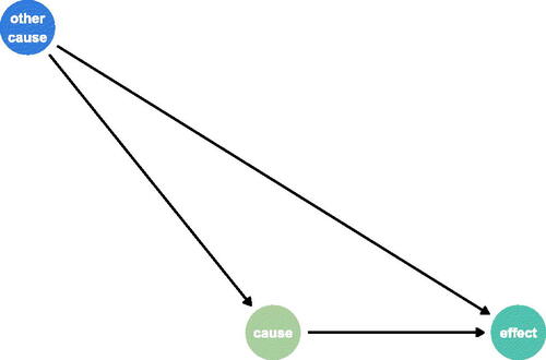
Directed acyclic graphs (DAGs) are a mechanism used to communicate causal relationships between factors. Factors are represented as nodes on the graphs, connected by directed edges (arrows). The edges point from causes to effects. The term acyclic refers to the fact that these graphs cannot have cycles. This is intuitive when thinking about causes and effects, as a cycle would not be possible without breaking the space-time continuum. DAGs are often used to communicate proposed causal relationships between a set of factors. For example, Figure 1 displays a DAG that suggests that the cause causes effect and other cause causes both cause and effect.

Fig. 1 Example DAG. Here, there are three nodes representing three factors: cause, other cause, and effect. The arrows demonstrate the causal relationships between these factors such that cause causes effect and other cause causes both cause and effect.

3.1 Causal Quartet

We propose the following four data generation mechanisms, summarized by the equations in Table 1, as well as the DAGs displayed in Figure 2. Here, X is presumed to be some continuous exposure of interest, Y a continuous outcome, and Z a known, measured factor. The M-Bias equation includes two additional, unmeasured factors, U₁ and U₂.

Fig. 2 Directed acyclic graphs describing the four data generating mechanisms: (1) Collider (2) Confounder (3) Mediator (4) M-Bias.

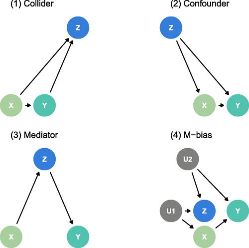
Table 1 Causal terminology along with the data generating mechanism for each of the four datasets included in the causal quartet.

Technical term	Explanation	Data generating mechanism
(1) Collider	The exposure, X, causes a factor, Z, and the outcome, Y, causes a factor, Z. Adjusting for Z when estimating the effect of X on Y would yield a biased result.	$X\sim N(0,1),Y=X+{\epsilon }_y,{\epsilon }_y\sim N(0,1)$ $Z=0.45X+0.77Y+{\epsilon }_z,{\epsilon }_z\sim N(0,1)$
(2) Confounder	A factor, Z, causes both the exposure, X, and the outcome, Y. Failing to adjust for Z when estimating the effect of X on Y would yield a biased result.	$Z\sim N(0,1),X=Z+{\epsilon }_x,{\epsilon }_x\sim N(0,1)$ $Y=0.5X+Z+{\epsilon }_y,{\epsilon }_y\sim N(0,1)$
(3) Mediator	An exposure, X, causes a factor, Z, which causes the outcome, Y. Adjusting for Z when estimating the effect of X on Y would yield the direct effect, not adjusting for Z would yield the total effect of X on Y. The direct effect represents the relationship between X and Y independent of any mediator, while the total effect includes both the direct effect and any indirect effects mediated by the potential mediator.	$X\sim N(0,1)$, $Z=X+{\epsilon }_z,{\epsilon }_z\sim N(0,1)$ $Y=Z+{\epsilon }_y,{\epsilon }_y\sim N(0,1)$
(4) M-Bias	There are two additional factors, U1 and U2. Both cause Z, U1 causes the exposure, X, and U2 causes the outcome, Y. Adjusting for Z when estimating the effect of X on Y will yield a biased result.	$U_1\sim N(0,1),U_2\sim N(0,1)$ $Z=8U_1+U_2+{\epsilon }_z,{\epsilon }_z\sim N(0,1)$ $X=U_1+{\epsilon }_x,{\epsilon }_x\sim N(0,1)$ $Y=X+U_2+{\epsilon }_y,{\epsilon }_y~N(0,1)$

In each of these scenarios, a linear model fit to estimate the relationship between X and Y with no further adjustment will result in an expected $\widehat{\beta }$ coefficient of 1. Or, equivalently, the expected estimated average treatment effect ($\widehat{\text{ATE}}$) without adjusting for Z is 1. The correlation between X and the additional known factor Z is also 0.70.

We have simulated 100 data points from each of the four mechanisms; we display each in Figure 3. This set of figures demonstrates that despite the very different data-generating mechanisms, there is no clear way to determine the “appropriate” way to model the effect of the exposure X and the outcome Y without additional information. For example, the unadjusted models are displayed in Figure 3, showing a relationship between X and Y of 1. The unadjusted models are the correct causal model for data-generating mechanisms (1) and (4); however, it overstates the effect of X for data-generating mechanism (2) and describes the total effect of X on Y for data-generating mechanism (3), but not the direct effect (Table 2). Even examining the correlation between X and the known factor Z does not help us determine whether adjusting for Z is appropriate, as it is 0.7 in all cases (Table 3). It is commonly suggested when attempting to estimate causal effects using observational data that the design step (i.e., selecting which variables to adjust for) should be separate from the analysis step (i.e., fitting an outcome model) (Rubin 2008). Even following the advice to choose which variables to adjust for without examining any outcome data can result in adjusting for factors that would lead to spurious estimates of the causal effect, as seen here where the correlation between X and Z is the same in every dataset even though adjusting for Z is sometimes not correct. Additionally, while it is not recommended to choose which factors to adjust using the outcome variable (as this can lead to increased Type 1 error and breaks the philosophical emulation of a randomized trial), if we examine the correlation between Z and Y, we find that it is positive in all four cases as well. Specifically, looking at the collider and confounder examples, the correlation between Z and Y is approximately the same (0.8) in the example datasets, and yet the confounder ought to be adjusted for and the collider not.

Fig. 3 100 points generated using the data generating mechanisms specified (1) Collider (2) Confounder (3) Mediator (4) M-Bias. The blue line displays a linear regression fit estimating the relationship between X and Y; in each case, the slope is 1.

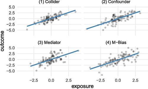
Table 2 Correct causal models and average causal effects for each data-generating mechanism.

Data generating mechanism	Correct causal model	Correct average causal effect
(1) Collider	Y ˜ X	1
(2) Confounder	Y ˜ X ; Z	0.5
(3) Mediator	Direct effect: Y ˜ X ; Z Total Effect: Y ˜ X	Direct effect: 0 Total effect: 1
(4) M-Bias	Y ˜ X	1

NOTE: The notation $X;Z$ implies that we should adjust for Z when estimating the causal effect. In other words, for the confounder data generating mechanism and direct effect mediator model, the potential outcomes are independent of exposure given the observed factor Z.

Table 3 Estimated average treatment effects under each data generating mechanism with and without adjustment for Z as well as the correlation between X and Z.

Data generating	$\widehat{\text{ATE}}$ not adjusting	$\widehat{\text{ATE}}$ adjusting	Correlation
mechanism	for Z	for Z	of X and Z
(1) Collider	1	0.55	0.7
(2) Confounder	1	0.50	0.7
(3) Mediator	1	0.00	0.7
(4) M-Bias	1	0.88	0.7

Each of the four datasets described above are available for use in the quartets R package (D’Agostino McGowan 2023). When using these datasets in the classroom, potential real-world examples could be assigned to the variables in line with the domain expertise of the students. For example, if the course were taught to medical professionals, the exposure, X, could be sodium intake, the outcome, Y, systolic blood pressure, and a collider, Z, urinary protein excretion (Luque-Fernandez et al. 2019). See the quartets package vignette titled “A collider example in a medical context” for an example of a lesson plan using this framework (D’Agostino McGowan 2023).

3.2 The Solution

Here we have demonstrated that when presented with an exposure, outcome, and some measured factors, statistics alone, whether summary statistics or data visualizations, are insufficient to determine the appropriate causal estimate. Analysts need additional information about the data generating mechanism to draw the correct conclusions. While knowledge of the data generating process is necessary to estimate the correct causal effect in each of the cases presented, an analyst can take steps to make mistakes such as those shown here less likely. The first is discussing understood mechanisms with content matter experts before estimating causal effects. Drawing the proposed relationships via causal diagrams such as the directed acyclic graphs shown in Figure 2 before calculating any statistical quantities can help the analyst ensure they are only adjusting for factors that meet the “backdoor criterion,” that is, adjusting for only factors that close all backdoor paths between the exposure and outcome of interest (Pearl 2000).

Absent subject matter expertise, the analyst can at least consider the time ordering of the available factors. Fundamental principles of causal inference dictate that the exposure of interest must precede the outcome of interest to establish a causal relationship plausibly. In addition, to account for potential confounding, any covariates adjusted for in the analysis must precede the exposure in time. Including this additional timing information would omit the potential for two of the three misspecified models above (Table 1, the “collider” and the “mediator”) as the former would demonstrate that the factor Z falls after both the exposure and outcome and the latter would show that the factor Z falls between the exposure and the outcome in time. For example, if we drew the second panel of Figure 2 (the Collider) as a time ordered DAG, we would see something like Figure 4. If we carefully adjust only for factors that are measured pre-exposure, we would not induce the bias we see in Table 3 (Figure 4(b)). The causal quartet datasets are accompanied by a set of four datasets with time-varying measures for each of the factors, X, Y, and Z, generated under the same data generating mechanisms. Here, as long as a pre-exposure measure of Z is adjusted for, the correct causal effect is estimated in all scenarios except M-Bias (Table 4). These datasets also serve the useful pedagogical purpose that since time is included in the information provided there are particular DAGs that are always incorrect. For example, an arrow between Z at follow-up and the X at baseline is impossible, since, as far as the authors are aware, time travel is not possible. That is, factors in the future cannot cause effects in the past.

Fig. 4 Time-ordered collider DAG (with time increasing from left to right) where each factor is measured twice. X is the exposure, Y is the outcome, and Z is the measured factor. The highlighted Z node indicates which time point is being adjusted for when estimating the average treatment effect of the highlighted X on the highlighted Y.

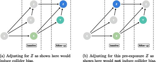
Table 4 Coefficients for the exposure under each data generating mechanism depending on the model fit as well as the correlation between X and Z.

Data generating mechanism	$\widehat{\text{ATE}}$ not adjusting for pre-exposure Z	$\widehat{\text{ATE}}$ adjusting for pre-exposure Z	Correct average causal effect
(1) Collider	1	1.00	1.0
(2) Confounder	1	0.50	0.5
(3) Mediator	1	1.00	1.0
(4) M-Bias	1	0.88	1.0

Adjusting for only pre-exposure factors is widely recommended. The only exception is when a known confounder is only measured after the exposure in a particular data analysis, in which case some experts recommend adjusting for it. Still, even then, caution is advised (Groenwold, Palmer, and Tilling 2021). Many causal inference methodologists would recommend conditioning on all measured pre-exposure factors (Rubin and Thomas 1996; Rosenbaum 2002; Rubin 2008, 2009). Including timing information alone (and thus adjusting for all pre-exposure factors) does not preclude one from mistakenly fitting the adjusted model under the fourth data generating mechanism (M-bias), as Z can fall temporally before X and Y and still induce bias. It has been argued, however, that this strict M-bias (e.g., as in Table 1 where U₁ and U₂ have no relationship with each other and Z has no relationship with X or Y other than via U₁ and U₂) is very rare in most practical settings (Rubin 2009; Gelman 2011; Liu et al. 2012). Indeed, even theoretical results have demonstrated that bias induced by this data generating mechanism is sensitive to any deviations from this form (Ding and Miratrix 2015).

4 Discussion

In the spirit of Anscombe’s Quartet, small datasets created to demonstrate a key concept akin to those we introduce here have been used for a wide variety of data analytic problems. Recent examples include an extension of the original idea proposed by Anscombe called the “Datasaurus Dozen” (Matejka and Fitzmaurice 2017), an exploration of varying interaction effects (Rohrer and Arslan 2021), a quartet of model types fit to the same data that yield the same performance metrics but fit very different underlying mechanisms (Biecek, Baniecki, and Krzyznski 2023), and a set of conceptual causal quartets that highlight the impact of treatment heterogeneity on the average treatment effect (Gelman, Hullman, and Kennedy 2023). While similar in name, the conceptual causal quartets are different from what we present here as they provide excellent insight into how variation in a treatment effect/treatment heterogeneity can impact an average treatment effect (by plotting the latent true causal effect). We believe both sets provide important and complementary understanding for data analysis practitioners.

We have presented four example datasets demonstrating the importance of understanding the data-generating mechanism when attempting to answer causal questions. These data indicate that more than statistical summaries and visualizations are needed to provide insight into the underlying relationship between the variables. An understanding or assumption of the data-generating mechanism is required to capture causal relationships correctly. These examples underscore the limitations of relying solely on statistical tools in data analyses and highlight the crucial role of domain-specific knowledge. Moreover, they emphasize the importance of considering the timing of factors when deciding what to adjust for.

Supplementary Materials

The supplementary material includes R code to generate the tables and figures.

Data Availability Statement

The causal quartet datasets presented in this article are available in an R package titled quartets (D’Agostino McGowan 2023). https://r-causal.github.io/quartets/

Disclosure Statement

No potential conflict of interest was reported by the author(s).

References

- Anscombe, F. J. (1973), “Graphs in Statistical Analysis,” The American Statistician, 27, 17–21. DOI: 10.2307/2682899.
- Biecek, P., Baniecki, H., and Krzyznski, M. (2023), “Performance Is Not Enough: A Story of the Rashomon’s Quartet,” arXiv preprint arXiv:2302.13356.
- D’Agostino McGowan, L. (2023), “quartets: Datasets to Help Teach Statistics,” availabe at https://github.com/r-causal/quartets; https://r-causal.github.io/quartets/.
- Ding, P., and Miratrix, L. W. (2015), “To Adjust or Not To Adjust? Sensitivity Analysis of M-bias and Butterfly-Bias,” Journal of Causal Inference, 3, 41–57. DOI: 10.1515/jci-2013-0021.
- Gelman, A. (2011), “Causality and Statistical Learning,” American Journal of Sociology, 117, 955–966. DOI: 10.1086/662659.
- Gelman, A., Hullman, J., and Kennedy, L. (2023), “Causal Quartets: Different Ways to Attain the Same Average Treatment Effect,” arXiv preprint arXiv:2302.12878. DOI: 10.1080/00031305.2023.2267597.
- Groenwold, R. H., Palmer, T. M., and Tilling, K. (2021), “To Adjust or Not to Adjust? When a “Confounder” Is Only Measured After Exposure,” Epidemiology (Cambridge, Mass.), 32, 194–201. DOI: 10.1097/EDE.0000000000001312.
- Hernán, M. A. (2012), “Beyond Exchangeability: The Other Conditions for Causal Inference in Medical Research,” Statistical Methods in Medical Research, 21, 3–5. DOI: 10.1177/0962280211398037.
- Imbens, G. W., and Rubin, D. B. (2015), Causal Inference in Statistics, Social, and Biomedical Sciences, Cambridge: Cambridge University Press.
- Liu, W., Brookhart, M. A., Schneeweiss, S., Mi, X., and Setoguchi, S. (2012), “Implications of M bias in Epidemiologic Studies: A Simulation Study,” American Journal of Epidemiology, 176, 938–948. DOI: 10.1093/aje/kws165.
- Luque-Fernandez, M. A., Schomaker, M., Redondo-Sanchez, D., Jose Sanchez Perez, M., Vaidya, A., and Schnitzer, M. E. (2019), “Educational Note: Paradoxical Collider Effect in the Analysis of Non-communicable Disease Epidemiological Data: A Reproducible Illustration and Web Application,” International Journal of Epidemiology, 48, 640–653. DOI: 10.1093/ije/dyy275.
- Matejka, J., and Fitzmaurice, G. (2017), “Same Stats, Different Graphs: Generating Datasets with Varied Appearance and Identical Statistics through Simulated Annealing,” in Proceedings of the 2017 CHI Conference on Human Factors in Computing Systems, pp. 1290–1294.
- Pearl, J. (2000), Causality: Models, Reasoning, and Inference, Cambridge: Cambridge University Press.
- Rohrer, J. M., and Arslan, R. C. (2021), “Precise Answers to Vague Questions: Issues with Interactions,” Advances in Methods and Practices in Psychological Science, 4, 25152459211007368. DOI: 10.1177/25152459211007368.
- Rosenbaum, P. (2002), “Constructing Matched Sets and Strata,” in Observational Studies, pp. 200–224, New York: Springer.
- Rubin, D. B. (1974), “Estimating Causal Effects of Treatments in Randomized and Nonrandomized Studies,” Journal of Educational Psychology, 66, 688–701. DOI: 10.1037/h0037350.
- ——- (2008), “For Objective Causal Inference, Design Trumps Analysis,” The Annals of Applied Statistics, 2, 808–840.
- ——- (2009), “Should Observational Studies be Designed to Allow Lack of Balance in Covariate Distributions Across Treatment Groups?” Statistics in Medicine, 28, 1420–1423.
- Rubin, D. B., and Thomas, N. (1996), “Matching Using Estimated Propensity Scores: Relating Theory to Practice,” Biometrics, 52, 249–264. DOI: 10.2307/2533160.