Earthquake-triggered landslides and Environmental Seismic Intensity: insights from the 2018 Papua New Guinea earthquake (M_w 7.5)

ABSTRACT

On the 25 February 2018, an earthquake of magnitude M_w7.5 struck the region of Porgera in Papua New Guinea (PNG), triggering numerous landslides. Planetscope images are used to derive a partial inventory of 2941 landslides in a cloud-free area of 2686 km². The average area of landslides in the study area is 18,500 m². We use the Environmental Seismic Intensity (ESI) scale to assess the damage due to the triggered landslides. Local intensity values are assigned to individual landslides by calculating their volume using various area–volume relations. We observe that different empirical relations yield similar volume values for individual landslides (local ESI intensity ≥ X). The spatial variation of landslide density and areal coverage within the study area in cells of 1 km² is investigated and compared to the probability predicted by the USGS model. We observe that high probability corresponds to a significant number of landslides. An ESI epicentral intensity of XI is estimated based on primary and secondary effects. This study represents the first application of the ESI scale to an earthquake in PNG. The Porgera earthquake fits well with past case studies worldwide in terms of ESI scale epicentral intensity and triggered landslide number as a function of earthquake magnitude.

KEYWORDS:

• Earthquake Environmental Effects (EEE)
• ESI scale 2007
• Papua New Guinea
• Earthquake-induced landslides

1. Introduction

Earthquake-induced landslides are caused by moderate to strong earthquakes in steep terrain. The sudden and rapid evolution of coseismic landslides is a significant threat to human settlements in their vicinity. Large earthquakes that have triggered thousands of landslides in the last two decades include the 2005 Kashmir earthquake, the 2008 Wenchuan earthquake, the 2015 Gorkha earthquake and the 2016 Kaikoura earthquake (Basharat et al., 2021; C. Massey et al., 2018; Roback et al., 2018; Xu et al., 2014). Some of the significant consequences caused by the triggered landslides are landslide dams, destruction of infrastructure and roadblocks. After an earthquake, landslide deposits can be remobilised by other processes such as aftershocks or heavy rainfall and relocated elsewhere. Compiling the inventories of earthquake-triggered landslides plays a vital role in creating predictive models. These models provide a rapid estimate of the spatial distribution of landslides in the aftermath of an earthquake (Bojadjieva et al., 2018; Harilal et al., 2019; Ramesh & M, 2012; Thambidurai & Ramesh, 2017). Two descriptors are generally used to analyse the spatial distribution of landslides, the landslide density and the landslide area percentage. Density and area percentage can then be explored with respect to topography, lithology and seismological or structural factors (Chang et al., 2021; Fan et al., 2018; Ling et al., 2021; F. Wang et al., 2019; Xu et al., 2018).

Spatial distribution of Earthquake-Induced Landslides (EQIL) is documented since large devastating events occurred (Keefer, 2002). The literature quantifies and predicts the eminent hazard by using available event-based inventories (Basharat, Rohn, Baig, et al., 2014b) (Tanyaş et al., 2022) (Velázquez-Bucio et al., 2023). The 2005 Kashmir earthquake of M_w 7.6 is a well-documented event that combines the inventory as well as field investigations that comprehensively explains the spatial distribution of the triggered landslides. Basharat et al. 2014b report that landslides mainly occurred on slopes of 30°−40° facing the Southern direction. The authors have reported that the landslide distribution is directly correlated with the distance from the triggering fault (Basharat, Rohn, Baig, & Khan, 2014a). Field studies in the affected areas revealed that hanging wall effect along the Muzaffarabad fault triggered landslides of large surface area during the Kashmir earthquake (Basharat, Rohn, Baig, et al., 2014b). Similarly, the landslides caused by the 1994 Northridge earthquake of M_W 6.8 is one of the many well-documented events that combine datasets from detailed geotechnical and geological investigations with an inventory that is by far the most complete inventory for the event (Harp & Jibson, 1996). Harp and Jibson (1996) surveyed the earthquake-affected areas using drone images and optical satellite images to delineate the slopes affected by the earthquake tremors. Albeit limited by the deficiency of advanced technology in the 90s, this event is still one of the benchmarks of a well-documented EQIL inventory. These inventories are necessary tools to investigate the causative factors and conduct detailed investigation on slopes that were triggered by earthquakes. Therefore, it is of prime importance to document an inventory of EQIL for various earthquake events (Tanyaş et al., 2017).

Landslides are one of the Earthquake Environmental Effects (EEEs) that can be categorised systematically by applying the Environmental Seismic Intensity (ESI) scale (Michetti et al., 2004) (Michetti A.M. et al., 2007) (Serva, 2019; Serva et al., 2016). The ESI scale assigns macroseismic intensity based exclusively on EEEs and is also applicable in sparsely populated regions. In the ESI framework, an individual landslide is a ‘site’ (i.e. a place where a single EEE is documented) and an ESI intensity value can be assigned to every site based on the mobilised volume. Volume may be estimated either from field surveys or by analysing the pre- and post-event digital elevation model (DEM) data (Chen et al., 2006; Corsini et al., 2009; Dewitte et al., 2008; Hsieh et al., 2016; Tarolli, 2014). Photogrammetric techniques that recreate the 3-D model of the study area and Lidar point cloud data may provide better volume estimates (Jaboyedoff et al., 2020; C. I. Massey et al., 2019). However, area–volume power laws are applied to arrive at volume estimates in the absence of such detailed datasets. Several such relations are proposed in the literature, with local or global validity while considering different types of slope movements (e.g. bedrock vs. shallow landslides) (Guzzetti et al., 2009; Larsen et al., 2010; Xu et al., 2016). Therefore, selecting the proper area–volume relation is an important step towards assigning the ESI intensity. An epicentral ESI intensity is assigned based on the dimensions of primary effects (length and offset of surface ruptures, amount of permanent ground deformation) or the extent of secondary effects (including landslides). Another study of the same event by Tanyaş et al. (2022) analysed the size distribution and the temporal evolution of the triggered landslides; however, it does not estimate the ESI intensity and the EEEs caused by this event.

Since its introduction, the ESI scale has been applied to over 150 recent and historical earthquakes worldwide (Esposito et al., 2013; Ferrario et al., 2022) – a database listing all the investigated events is publicly available (see ‘Availability of data’ section). Some of the case histories specifically dealing with the ESI assessment of slope movements include the 1976 Guatemala, 1998 Krn (Slovenia), the 2003 and 2015 Lefkada (Greece) and the 2011 Lorca (Spain) earthquakes (Caccavale et al., 2019; Gosar, 2012; Papathanassiou & Pavlides, 2007; Papathanassiou et al., 2017; Silva et al., 2013). Ota et al. analysed several earthquakes in Japan and Taiwan to assign the ESI intensity. The authors analysed the EEEs due to earthquakes over a grid in the study area and evaluated the intensity in each cell of equal dimensions. Their results suggest that the ESI scale can capture the morphological changes observed in the study area after a major earthquake event (Ota et al., 2009). These morphological changes combined with the spatial distribution of landslides give an overview of the coseismic landslide hazard in any investigated terrain.

In this work, we investigate the landslides triggered by the 25 February 2018 Porgera earthquake in Papua New Guinea (PNG) with a moment magnitude M_w 7.5. We generate and analyse a partial inventory and assess the spatial distribution of landslides using the landslide number density (LND) and the landslide area percentage (LAP). The variation in normalised landslide density in the study area is compared to the probability map as predicted by the USGS ground failure model (Nowicki Jessee et al., 2018). Based on our calculations, we assign an ESI epicentral intensity of XI after evaluating different descriptors (primary surface rupture, permanent ground deformation, area affected by secondary effects). The Porgera case history is compared with various thrust fault events worldwide, and a good correlation between ESI epicentral intensity and the number of triggered landslides is evident. The workflow used here assigns ESI directly from EQIL mapping and can be applied to future earthquakes that trigger landslides. We would also like to stress that this is the first time the ESI index has been applied for a case history in the PNG islands. This work addresses three main research questions.

1. Building of a partial inventory of the landslides triggered by the 2018 Porgera earthquake.

2. Documenting the EEEs and assigning the ESI epicentral intensity for the event.

3. Assessing the spatial distribution of triggered landslides from the mapped inventory to enhance the understanding of EQIL and their contribution to EEEs caused by the earthquake.

Regional geological setting and the Porgera earthquake

The M_w 7.5 Porgera earthquake occurred on 25 February 2018, at a depth of 25.2 km. The epicentre is located at 6.070°S 142.754°E, in a sparsely populated region 32 km SW of Tari (USGS, 2019). The earthquake originated from a thrust fault due to the oblique convergence between the Australian plate over the Pacific plate (Figure 1a), which moves with a velocity of ca. 110 mm/yr, mainly accommodated by the offshore trench. The onshore faults, including the Papuan Fold and Thrust Belt (PFTB), where the 2018 Porgera epicentre is located, accommodate a portion of the plate motion, with rates varying along-strike (Koulali et al., 2015).

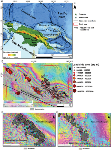
Figure 1. a) Regional map of the study area with tectonic boundaries, mainshock and aftershock locations (Basemap courtesy NOAA). The area within the red box is enlarged in (b). b) Porgera earthquake epicenter and location of the mapped landslides represented as points that correspond to their size. The red box is the extent of the study area mapped for landslides. The base map of the study area is the interferogram of the earthquake obtained from: https://www.gsi.go.jp. c) and d) Sample of landslide polygons in the study area. It can be seen that these polygons correspond to the decorrelated parts of the interferogram.

Since 1900, the largest event recorded in the PFTB is the Porgera earthquake. Close observation of the fault geometry and slip distribution using seismological, GPS and InSAR data reveals a complex pattern involving the rupture of several segments (Mahoney et al., 2021; S. Wang et al., 2020; Zhang et al., 2020). In the months following the M_w 7.5 mainshock, several aftershocks with M_w >6 were recorded (Zhang et al., 2020). Ground deformation following the Porgera earthquake affected an area of ca. 7500 km², with a maximum uplift of 1.2 m (Mahoney et al., 2021). Surface rupture was documented using sub-pixel offset measurements with vertical and horizontal displacements of 2 m and 4.3 m (Chong & Huang, 2021).

Figure 1b shows the interferogram obtained from ALOS-2/PALSAR-2 data where each coloured fringe represents 12 cm of movement between the ground and the satellite measured along the Line of Sight (LOS). The decorrelation in InSAR data suggests the occurrence of extensive coseismic slope movements triggered by the Porgera earthquake. Nevertheless, persistent cloud cover after the event hampered the realisation of an EQIL inventory immediately after the event. The earthquake sequence was preceded, accompanied and followed by heavy rainfall, which further triggered landslides and made the landslide mapping an onerous task. Tanyaş et al. (2022) mapped over 10,000 slope movements, investigating the role of seismicity, geology, topography and high rainfall (Tanyaş et al., 2022). The Porgera earthquake was included as a case history in HazMapper, an open-access application based on Google Earth Engine characterising the effects of natural disasters (Scheip & Wegmann, 2021).

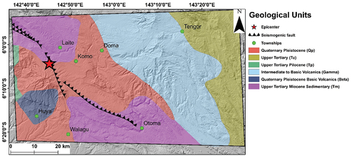
Systematic geological mapping of New Guinea was started in the 1960s albeit the earliest geological exploration began in the 1800s. The geological setting of New Guinea reveals the effect of compression between the Indo-Australian plate and Pacific plates. As seen in Figure 1a, the study area is part of the PFTB which adds to the fragility of the geological formation in the region as there is constant plate motion along the thrust belt. Volcanic Arc and Ophiolite formations are the common units observed in the uplift process in the island, which are fractured by transcurrent faulting and rifting (Pieters, 1982). We adopted the geological map obtained from the PNG geological survey as shown in Figure 2. The regional geological succession of the study area and its surroundings is characterised by Tertiary age sedimentary and metamorphic rocks from the Miocene epoch overlain by Quaternary deposits. There are notable intrusions of intermediate to Basic volcanic rocks with traces of Quaternary Pleistocene rocks. Sandstone, conglomerate, limestone, shale and siltstone formed in the late Palaeozoic and Mesozoic eras are found evenly distributed in the region. Deformed volcanics from the same age are also observed as a result of block faulting and gravitational folding. Rare fossils in oldest dated rocks are from the Cretaceous period (Pieters, 1982). The newer undeformed volcanics and sediments comprise the quaternary beds (Tanyaş et al. 2022).

Figure 2. Geological map of the study area (source PNG geological survey). Fault trace adapted from S. Wang et al. (2020).

The island of New Guinea is known for gold and silver mines. Gold was first found on the island in 1852 and the hunt for more of the lucrative metal started around this time. The mines have been active since the late 90s to early 2000s. The Porgera gold mine is the closest to the study area. The operational mines also contribute to slope instability in various parts of the island (Singh, 2010). Ground shaking and environmental effects of past earthquakes are witnessed by the mine workers and have been reported to be disastrous for the miners (Singh, 2010).

3. Methodology

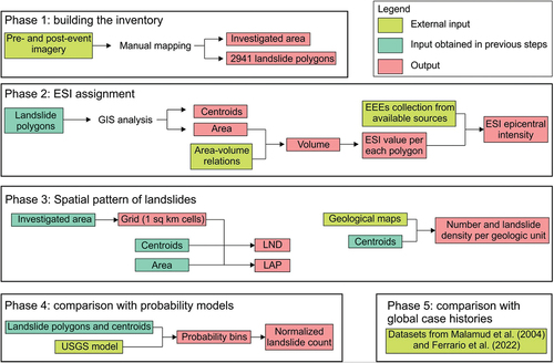
We follow a rigorous workflow, comprising a multi-step procedure. The methodological framework involves the exploitation of external inputs (e.g. satellite images), their analysis and derivation of original products; such products are then used to proceed to further steps in the analysis, with the final aim of documenting the overall damage through the analysis of EEEs. Figure 3 presents the flow chart of the methodology followed in this work: the first step is the building of the landslide inventory from satellite images. Phase 2 comprises the core of the work, which is the assignment of ESI local and epicentral values. This step involves GIS analysis of the mapped landslide polygons, supplemented with area–volume relations and the collection of other EEEs from the literature. In Phase 3, we evaluate the distribution of landslides, obtaining the LAP and LND maps and correlating landslides with geological units in the study area. Finally, Phases 4 and 5 move towards a generalisation: in particular, we compare the spatial distribution of mapped landslides with the predicted spatial probability calculated by the USGS model to give an overview of spatial distribution of landslides (Phase 4). Phase 5 compares the Porgera case study with other earthquakes worldwide.

Figure 3. Flow chart of the methodology followed in this work with hierarchy of steps used to carry out the scientific investigation.

3.1. Realization of the landslide inventory

Multispectral Planet labs imagery from 13 January to 27 March 2018 is used for mapping the landslide polygons. The pre- and post-event images for an area of 2686 km² are visually monitored. To increase the quality of the inventory and capture surface changes caused by slope failures, individual landslides are mapped as polygons rather than points (Harp et al., 2011). The Planet Labs imagery’s 3 m/pixel resolution precisely delineates the area subjected to landslides (Sridharan et al., 2020). The pre-images as early as the 22 February are used for comparison, given the earthquake occurred on the 25 February. However, due to cloud cover in the satellite images for some parts of the study area on the 22 February, images from the 13 January and the 4 February had to be compared with the post-images to eliminate the possibility of mapping retriggered landslides. Coalescing landslides with multiple source points identified in the study area are mapped as individual polygons. To further confirm such coalescence, post-images obtained on 4 March are used as this can possibly show us the toe of each landslide. Albeit the satellite images were heavily clouded on 4 March, gaps in the clouds revealed certain areas that experienced landslides.

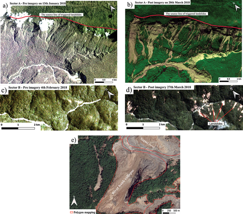
Apart from freshly triggered and retriggered landslides, riverbank collapses, as shown in Figure 4e, are also observed. The number of landslides per unit area (i.e. landslide density) and landslide area percentage are calculated to estimate the spatial distribution of landslides. Landslide centroids are extracted from the polygons, and the analysis is performed on a grid with 1 km × 1 km resolution. Mapped landslides lie within the deformed area of the interferogram shown in Figure 1a.

Figure 4. a) Pre-event images of Sector a captured on 13 January 2018. b) Post-event images of Sector A, taken on 20 March 2018. c) Pre-event image of Sector B captured on 4 February 2018. d) Post-event image of Sector B taken on 27 March 2018 (see Figure 5 for locations and lat-long details of the sectors). e) Shows an example of riverbank collapse along Tagiri River acquired from Google earth (2018) imagery post the earthquake.

Among various models that predict the spatial distribution of landslides after an earthquake, the USGS Jesse et al. (Nowicki Jessee et al., 2018) model is frequently used in predicting the probability of landslides. Nowicki Jessee et al. (2018) have proposed a logistic regression model among the probability, slope, peak ground velocity (PGV), land cover, compound topographic index (CTI) and lithology. Probability is the predicted variable, and the other terms are the independent variables (Nowicki Jessee et al., 2018). The raster of the probabilities for the study area is downloaded from the USGS event page for the Porgera earthquake (see ‘Availability of data’ section). The raster file of the probability values predicted for the event is converted to a vector layer with small squares with equal-area, called bins. We count the Centroids of the mapped landslide polygons in each probability bin with incremental probability values of 0.005, as this is the lowest significant digit in the range of probability values estimated by the USGS model. To normalise the count, we divide the number by the total area of the bins for each probability value. Adding up the area of individual bins with the same probability gives the total area covered by each probability value. The normalised density of landslides is compared with the probability values predicted by Jesse et al. (Nowicki Jessee et al., 2018). A possible limitation of this approach is that we consider landslide centroids, which may be facile for large failures.

3.2. Area–Volume conversion and ESI scale assignment

The conversion from mapped area to volumes is necessary to assign ESI intensity values. Among the scaling relations proposed in the literature (e.g. (Guzzetti et al., 2009; Jaboyedoff et al., 2020; Xu et al., 2016), several models use a power-law functional form. Other parameters such as Peak Ground Acceleration (PGA), slope aspect and slope can be considered for the area volume relation. However, the relation between the surface area and the volume is consistent with the power-law (Xu et al., 2016). In this paper, we evaluate different area–volume scaling relations for the mapped landslides, which have the general form:

(1) $\mathrm{V}={\alpha }^{\ast }{\mathrm{A}}^{\mathrm{Y}}$(1)

Where V is the volume (in m³), A is the area (in m²), ‘α’ and ‘γ’ are fitting coefficients. Selecting the most appropriate relation is not straightforward, and volume estimations may vary significantly. We tested different scaling relations (Guzzetti et al., 2009; Larsen et al., 2010; C. I. Massey et al., 2019; Simonett, 1967; Xu et al., 2016) to assess the influence of such a choice on the ESI intensity assignment. The ‘α’ and ‘γ’ coefficients of Equation 1(1) $\mathrm{V}={\alpha }^{\ast }{\mathrm{A}}^{\mathrm{Y}}$(1) show slight differences for soil and bedrock landslides, and a trend of increasing ‘α’ when ‘γ’ decreases is pointed out (Jaboyedoff et al., 2020). Simonett (1967) derived a local relation based on 207 landslides in central New Guinea. Guzzetti et al. (2009) analysed 677 worldwide landslides of predominantly slide type, including the New Guinea landslides of Simonett (1967). Nevertheless, the majority of the landslides are triggered by rainfall. Larsen et al. (2010) used 4231 individual landslides globally to derive volume-area scaling of bedrock and soil landslides. Xu et al. (2016) propose optimised models for area–volume conversion by analysing a subset of the landslides triggered by the 2008 Wenchuan earthquake. C. I. Massey et al. (2019) estimated source volumes for 17,256 landslides triggered by the 2016 Kaikoura (New Zealand) earthquake using a 2 m resolution vertical difference model. One of the most challenging tasks in estimating the volume of the landslides from the field to develop area volume power laws arises from estimation of the average depth. Due to the unavailability of pre-event characteristics of triggered landslides, the estimated post-event depth might not be accurate. On the other hand, the procedure to estimate the average depth varies among different investigators. These are the two main contributors to the error in estimating the power law exponent. The range of ‘γ’ for available power law models is 0.79 to 1.95 from literature (Ju et al., 2023). Initial models proposed by Keefer correlated the magnitude of triggering event to the volume of landslides and arrived at a power law relation based on 15 EQIL events. The relation between magnitude and volume gives erroneous results in the estimation of the landslide volumes as observed by several subsequent case studies. With the availability of high-resolution images and more sophisticated drones that acquire precise field images, the area volume power laws developed in the recent decades provide a more reliable estimate of landslide volume (Ju et al., 2023; Xu et al., 2016).

The ESI intensity is estimated following the description included in the scale (Michetti et al., 2004) as summarised in Table 1. Landslides start to occur in susceptible zones with ESI as low as IV, become significant from ESI VI and saturate at ESI X. It can be observed that the description does not change for intensity higher than X (Table 1). The selection of a given area–volume relation is a source of epistemic uncertainty. Recently, Ferrario (2022) demonstrated that the use of different area–volume relations has a negligible influence on the resulting ESI assessment, while a much higher influence is given by the quality of the input data, i.e. the landslide inventory itself.

Table 1. Summary of the characteristics of earthquake-triggered landslides and related ESI intensity. Modified after Michetti et al (2004, 2007).

ESI degree	Description	Typical volume
IV	Exceptionally few and small slope movements on unstable slopes
V	Rare, small slope movements
VI	Slope movements may occur in unstable zones	103 m^3
VII	Scattered slope movements in prone areas	103–105 m^3
VIII	Slope movements are widespread in prone areas. Landslides can dam narrow valleys	103–105 m^3
IX	Slope movements are widespread and can dam valleys	105–106 m^3
X	Frequent large slope movements, regardless of the state of equilibrium	>105–106 m^3
XI	Frequent large slope movements, regardless of the state of equilibrium, up to 200–300 km from the epicentre	>105–106 m^3
XII	Frequent large slope movements, regardless of the state of equilibrium, up to 200–300 km from the epicentre	>105–106 m^3

4. Results

4.1. Spatial distribution of earthquake-triggered landslides

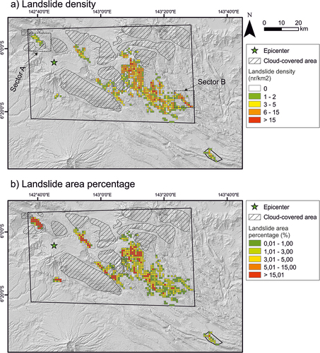
A total of 2941 landslides have been mapped in the study area. Most of the triggered landslides are along valleys with steep slope values of 55°–70°. We computed the area of each landslide in GIS software. By summing the individual landslide areas, a value of 54.37 km² is obtained, corresponding to ca. 2% of the total cloud-free investigated area. By dividing 54.37 km² by the number of mapped landslides, we obtain an average landslide area of 18,500 m². The mapped inventory contains five landslides belonging to a cluster of large landslides mapped in a small region to the NW of the epicentre, which we name sector A. These landslides have a surface area greater than 0.9 km² and account for 10% of the total landslide area. Similarly, sparse distribution of landslides with dimensions smaller than those mapped in sector A is observed in the NE corner of the study area, which we name sector B. An example of pre- and post-event images is shown in Figure 4. Images from the first week of February 2018 show no pre-existing landslides (Figure 4 b, d). The post-event images, captured in the period of 20–27 March 2018, reveal several landslides with source areas coalescing at the base of the slope (Figure 4 a).

Figure 5 shows the landslide density and landslide area percentage. Within the study area, maximum density values reach 36 landslides/km² and the maximum area percentage is 75%. The eastern and central parts of the investigated area have the highest values in terms of landslide density, while the high values of area coverage are more widespread. Two extreme cases of LND and LAP are observed in the mapped region. On the one hand, large complex landslide bodies are observed to cluster in small regions. On the other hand, many small landslides are distributed in a wide area. These cases are illustrated in Figure 5; in Sector A, 37 individual landslides are mapped. LND reaches a maximum value of 5 landslides/km², which is relatively low. On the contrary, LAP in Sector A (Figure 5a and b) reaches values of up to 67%, which is among the highest documented in the whole region. In sector B (Figure 5c and d), LND is as high as 36 landslides/km² and LAP is less than 8%, completely contrasting with the values observed in sector A.

Figure 5. a) Landslide Number Density (LND) and b) Landslide Area Percentage (LAP), computed on a 1-km² grid. Dashed boxes are enlarged in Figure 4 (Basemap: Digital Elevation Model (DEM) derived from ALOS data.).

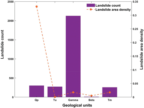
The correlation between landslide number and landslide area density in each geological unit is presented in Figure 6. For the landslide area density, the total area of all the landslides in each geological unit is divided by the area covered by that geological unit in the study area. Landslide number and landslide area per each geological unit show a different trend, suggesting that lithology plays a role in defining the average dimension of the triggered movements. Most landslides are observed in Intermediate to Basic volcanic rocks (Gamma); however, the maximum area was triggered in the Quaternary Pleistocene (Qp) rocks. Landslides with significantly larger areas are observed in the study area in Qp, as these are more recent deposits and contain fragile formations such as limestone. From Figure 6, the landslide area density in Basic volcanic rocks is very low, indicating a large number of small landslides were triggered in the volcanic rocks.

Figure 6. Variation of landslide count and area density in each geological unit present inside the study area.

4.2. ESI intensity assessment

Figure 7a shows seven power-law relations on a log–log plot of area and volume. For each relation, we calculated the area corresponding to a volume of 10⁶m³, which represents ESI intensity ≥ X. Values range between 73,000 and 285,000 m² for all the equations except Larsen et al. (2010) relation for soil landslides (value of 570,000 m²). Out of the 2941 landslides, 1% to 4% have an ESI value ≥ X (the value lowers to 0.3% if the soil-type equation by Larsen et al., 2010 is used). Slope movements saturate at ESI X, which means that it is not possible to assess degrees higher than X based on the volume of individual landslides (see Table 1).

Figure 7. a) Log–log plot of area–volume for various relations proposed in the literature. b) Frequency distribution of landslide area. c) Plot of the cumulative frequency of landslide volumes and relation with ESI intensity; the all-type Larsen et al. (2010) scaling relation is shown as an example. A similar relation is observed using all the equations illustrated in the box in the upper right corner.

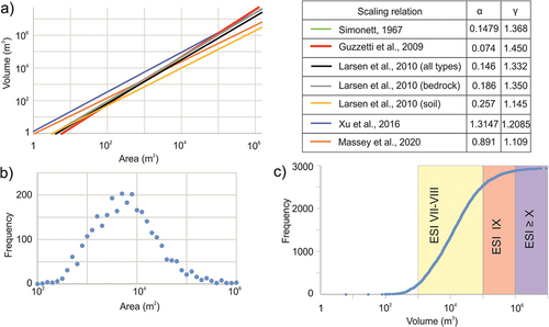
Figure 7b is a plot of the frequency–area curve for the mapped inventory. The variation obeys a positive power law for small landslides and a negative power law for large landslides. The highest point in the frequency area relation is termed ‘rollover’, which can estimate the minimum landslide size at which the inventory is nearly complete (Tanyaş & Lombardo, 2020). For our inventory, the rollover value is found to be 5000 m², which is relatively high but is within the range of rollover values observed by similar studies (Tanyaş & Lombardo, 2020).

Figure 7c shows the frequency of landslides according to their volume and the distribution in terms of ESI intensity values. The area–volume relation proposed by Larsen et al. (2010) is an equation with global validity and is shown as an example in the figure. A similar relation is observed for the other area–volume relations considered in this study. The selection of the area–volume scaling relation does not affect the assigned ESI intensity value based on the dimension of the largest slope movements. It is worth noting that ESI degrees and intensity scales, in general, are a classification system rather than the measurement of some physical parameter. In this sense, the ESI guidelines provide broad categories in terms of volume estimates (see Table 1). Since remote sensing datasets allow the generation of landslide inventories after an earthquake event, a quick way to convert areas to ESI intensity may be helpful in assessing the impact of the event.

The integration of EQIL mapping and ESI estimation has the additional advantage of estimating the intensity in remote or sparsely populated regions, where traditional intensity scales based on damage to the built environment cannot be applied. For the Porgera earthquake, sparse intensity data points are available from the ‘Did You Feel It?’ (DYFI) program, which uses online questionnaires to collect reports and information on earthquake damage. Intensity is provided in the Community Decimal Intensity (CDI) scale (Jay Wald et al., 2012). No intensity points are located in the first 30 km from the epicentre, and the highest CDI value is recorded at Tari, 32 km NE from the epicentre, with an intensity of 9.0. In remote locations, DYFI data provide sparser information with respect to the ESI scale. For the Porgera earthquake, CDI is lower than the ESI epicentral intensity, similar to what was observed for the 2018 Lombok, Indonesia, sequence (Ferrario, 2019).

The ESI epicentral intensity can be estimated from different metrics, such as the primary effects (surface faulting and permanent ground deformation) or the dimension of the area affected by secondary effects. Table 2 summarises the results obtained from the Porgera earthquake. The area encompassing all the landslides by the complete inventory (Tanyaş et al., 2022) is ca. 24,000 km² wide, pointing to ESI XI. Coseismic surface faulting with length in the order of 40 km and metric displacement was documented using subpixel offset tracking (Chong & Huang, 2021) and these values are consistent with ESI XI.

Table 2. ESI epicentral intensity of the Porgera earthquake as obtained from different descriptors, including primary and secondary effects. The ESI epicentral intensity as estimated in this study is XI.

Type of coseismic effect	Maximum value	ESI epicentral intensity
Volume of individual landslides	>10^6 m^3	≥X
Area affected by landslides	24,000 km^2	XI
Surface rupture length	40 km	X
Uplift from InSAR	1.2 m	X

Permanent ground deformation imaged by InSAR (Mahoney et al., 2021) shows a maximum uplift of ca. 1.2 m, which points to ESI X. Intensity assigned from permanent ground deformation has the lowest value among those reported in Table 2 and this can be possibly ascribed to the 25 km depth of the earthquake. Finally, the total area affected by permanent ground deformation is 7500 km² (Mahoney et al., 2021). Currently, this metric is not explicitly considered for ESI assignment, but we envisage that it could be a valuable addition to the ESI toolbox. Overall, we assign an epicentral intensity of XI on the ESI scale.

5. Discussion

Our research allowed us to build a partial landslide inventory and to analyse the spatial distribution of landslides using simple metrics such as Landslide Density Number (LND) and Landslide Area Percentage (LAP) on a regular grid. Additionally, we focus on macro-seismic intensity, which by definition is the documentation of earthquake effects. In particular, we inspect the effect on the natural environment, and we apply for the first time in PNG, the ESI scale. Given the high seismicity rate, the frequent occurrence of powerful earthquakes in the region and the relatively low population density, EEEs provide a sound alternative for documenting earthquake damage. We now move towards a generalisation (Phases 4 and 5 in the flow chart of Figure 3), by comparing our results with the probability model derived by the USGS (Section 5.1) and with global case histories, either in terms of other EQILs (Section 5.2) or earthquakes analysed using the ESI scale (Section 5.3).

5.1. Comparison of the inventory with the predicted landslide distribution

Figure 8 shows the normalised density with the corresponding predicted probability values. The highest probability value predicted by the USGS model, which is 0.25, is predicted in small patches within the study area. Remarkably high values in the range of 0.25 to 0.2 are observed in sector A.

Figure 8. Variation in normalised landslide density as a function of the probability values predicted by (Jessee et al., 2018). The density is calculated for bins with incremental probability values of 0.005. The procedure for calculating the normalized density is mentioned in section 3.1.

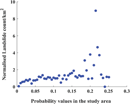
The plot in Figure 8 shows a gradual increase in the normalised landslide density up to a probability of 0.15, followed by a sudden increase beyond a probability of 0.18. This indicates that the bins with higher probability values should have a significant number of landslides. In sector B, the highest probability value observed is 0.174. As mentioned earlier, the landslides in sector B have a characteristically smaller surface area when compared to those in sector A. This also suggests that the volume of landslides based on power-law estimates correlates with the probability values predicted by the USGS model. For example, in sector A, the predicted probability values reach 0.23 and the volume estimates of individual landslides have a maximum value of 0.1479 km³. Similarly, in sector B, for probability values of 0.174, the maximum value of volume observed is 0.0006 km³. To assess if the drastic variations observed for Sectors A and B are exceptional or if such variability is common, it is necessary to realise similar comparisons for a larger dataset globally. Overall, the models developed for predicting near real-time hazards, such as the USGS model, have a crucial role in providing reliable estimates of the spatial distribution of the landslides. Nevertheless, it is observed that they do not give a reliable estimate of the landslide number or the area density (Burrows et al., 2021).

5.2. Spatial distribution of earthquake triggered landslides: comparison of the Porgera event with global case histories

Some valuable insights can be gained by comparing the Porgera partial inventory with global events. The average area of individual landslides in our inventory is 18,500 m², which is of the same order of magnitude as the more complete inventory realised by Tanyaş et al. (2022). They mapped 10,403 earthquake-triggered landslides that cover 145 km² (145 × 10⁶ m²), resulting in an average area of 13,940 m². Average areas derived from all available inventories in the history of EQIL cover a wide range of values between 200 and over 70,000 m² (Tanyaş et al., 2017). In Papua New Guinea, other than the 2018 Porgera earthquake, an EQIL inventory is available for the M_w 6.9 1993 Finisterre earthquake (Meunier et al., 2008). That event caused 4790 landslides covering a total area of 69 km², which means the average area per polygon is 14,405 m². This figure is remarkably similar to the Porgera earthquake, suggesting that the local climatic and topographic setting might contribute to the landslide dimension. Topographic site effects favour landslide clustering along inner gorges as documented for the 1993 Finisterre earthquake (Meunier et al., 2008) and are also observed for the Porgera earthquake (Mahoney et al., 2021).

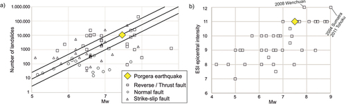
The largest landslide event ever documented is the 2008 Wenchuan earthquake (1159 km²), followed by the Porgera event (145 km² total triggered area). Other events that triggered landslides with a cumulative area of over 100 km² were the 1999 Chi-Chi, the 2002 Denali and the 2005 Kashmir earthquakes (Tanyaş et al., 2017). It is worth mentioning that, except for the Denali earthquake, all the others had a reverse focal mechanism. Figure 9apresents a graphical summary of the comparison between the Porgera earthquake and global case histories with respect to the number of triggered landslides. A total of 10,403 landslides triggered by the Porgera earthquake (Tanyaş et al., 2022) are along the empirical fit derived by Malamud et al. (2004). The style of faulting and displacement along the surface ruptures is found to be major contributors to the number of landslides as much as the magnitude (Xu, 2014). Reverse-fault earthquakes usually generate a higher number of landslides when compared with strike-slip and normal faulting events (Figure 9a).

Figure 9. a) The number of triggered landslides versus M_w for 65 events worldwide (modified after (Livio & Ferrario, 2020)). The empirical correlation and error bounds adopted from Malamud et al. (2004) are shown as solid lines. b) ESI epicentral intensity versus M_w for a dataset of 47 earthquakes with reverse/thrust mechanisms worldwide.

5.3. ESI intensity assessment: comparison of the Porgera event with global case histories

Figure 9b presents 47 earthquakes with reverse/thrust focal mechanisms, including the Porgera event analysed using the ESI scale. The dataset includes events from various seismotectonic settings such as subduction zones, continental collision and stable continental regions. The earthquakes range in magnitude between M_w 4.2 and M_w 9.0 and have variable depths up to ca. 35 km. The ESI epicentral intensity varies between VII and XII. It is worth noting that three events reached the maximum intensity of XII (Lekkas, 2010; Sanchez & Maldonado, 2016; Serva et al., 2016), while several earthquakes show an ESI intensity of XI. The Porgera earthquake fits well in the plot with previous case histories. ESI epicentral intensities of XI are found for earthquakes ranging in magnitude between 7 and 8.8, while earthquakes of M_w 7.5 (like the Porgera event) have epicentral intensity between VIII and XI. The data shown in Figure 9b reaffirm the reliability of ESI assessment and its consistency in estimating the hazard in different seismotectonic settings.

6. Conclusion

We have generated a partial inventory of the M_w 7.5 Porgera earthquake in PNG, containing 2941 landslides. Area–volume power laws are used to obtain the mobilised volume of individual landslides, which is then used to assign ESI local intensity with maximum values higher than X. An ESI epicentral intensity of XI is assigned based on the dimension of the area affected by secondary effects. This study represents the first application of the ESI scale to a PNG earthquake. The USGS spatial prediction model is fairly accurate in predicting the actual landslide distribution. The Porgera earthquake was compared with global case histories, and a good concurrence among ESI epicentral intensity and number of triggered landslides with respect to moment magnitude was documented.

The Porgera earthquake caused thousands of landslides in a remote and rugged region, making it an ideal candidate for the ESI scale. Mapping earthquake-induced landslides from satellite imagery is an efficient way to document the overall earthquake damage. This study is limited by the availability of cloud-free satellite images on the dates close to the day of the earthquake event and the time required to manually map the inventory, both of which are not feasible for emergency response. Additionally, we did not realise field surveys for the region. However, it demonstrates how to integrate the realisation of EQIL inventories with the assessment of ESI intensity into a single workflow. We observed that the local ESI intensity could be consistently estimated even by adopting different area–volume relations. The documentation of EEEs in this study is restricted to mapping the slope movements. The event could have caused other EEEs, but we believe that the estimated value of the ESI epicentral intensity is reliable since various metrics provide a consistent estimate. We suggest that the scientific communities dealing with compiling EQIL inventories and intensity estimation through the ESI scale can benefit from each other. On the one hand, the high resolution of EQIL inventories depicts the spatial variation of coseismic effects and potentially provides a detailed ESI macroseismic field. On the other hand, the ESI scale compares landslides with other earthquake environmental effects and compares different events on various temporal or spatial scales. This study on the Porgera earthquake can be replicated for other events. The realisation of landslide inventories is a fundamental prerequisite for further studies aimed at better estimating the seismic risk. This can further aid in developing more accurate predictive models for earthquake-induced landslides, to be put at use by local and regional authorities. Future research should include the analysis of causative factors and subsequent susceptibility mapping. These efforts are ultimately devoted to the minimisation of earthquake losses, either in terms of human lives or economic assets.

Availability of data

PlanetScope imagery was provided by Planet as part of their Educational and Research programme. The interferogram of the earthquake has been supplied by Japan GSI: https://www.gsi.go.jp/cais/topic180301-index-e.html. The data used for Figure 9a are extracted from https://zenodo.org/record/5520951#.YWVDMB zOM2w. USGS data on the Porgera earthquake can be accessed at https://earthquake.usgs.gov/earthquakes/eventpage/us2000d7q6/executive.

Disclosure statement

No potential conflict of interest was reported by the author(s).

Additional information

Funding

This work was not funded by any government or private organisations.

References

- Basharat, M., Riaz, M. T., Jan, M. Q., et al. (2021). A review of landslides related to the 2005 Kashmir Earthquake: Implication and future challenges. Natural Hazards, 108(1), 1–30. https://doi.org/10.1007/s11069-021-04688-8
- Basharat, M., Rohn, J., Baig, M. S., & Khan, M. R. (2014a). Spatial distribution analysis of mass movements triggered by the 2005 Kashmir earthquake in the Northeast Himalayas of Pakistan. Geomorphology, 206, 203–214. https://doi.org/10.1016/j.geomorph.2013.09.025
- Basharat, M., Rohn, J., Baig, M. S., Khan, M. S., & Schleier, M. (2014b). Large scale mass movements triggered by the Kashmir earthquake 2005, Pakistan. Journal of Mountain Science, 11(1), 19–30. https://doi.org/10.1007/s11629-012-2629-6
- Bojadjieva, J., Sheshov, V., & Bonnard, C. (2018). Hazard and risk assessment of earthquake-induced landslides—case study. Landslides, 15(1), 161–171. https://doi.org/10.1007/s10346-017-0905-9
- Burrows, K., Milledge, D., Walters, R., & Bellugi, D. (2021). Improved rapid landslide detection from integration of empirical models and satellite radar. Natural Hazards and Earth System Sciences, 1–34. https://doi.org/10.5194/nhess-2021-148
- Caccavale, M., Sacchi, M., Spiga, E., & Porfido, S. (2019). The 1976 Guatemala earthquake: ESI Scale and probabilistic/deterministic seismic hazard analysis approaches. Geosciences, 9(9), 403. https://doi.org/10.3390/geosciences9090403
- Chang, M., Zhou, Y., Zhou, C., & Hales, T. C. (2021). Coseismic landslides induced by the 2018 Mw 6.6 Iburi, Japan, Earthquake: Spatial distribution, key factors weight, and susceptibility regionalization. Landslides, 18(2), 755–772. https://doi.org/10.1007/s10346-020-01522-3
- Chen, R. F., Chang, K. J., Angelier, J., Chan, Y. C., Deffontaines, B., Lee, C. T., Lin, & M. L. (2006). Topographical changes revealed by high-resolution airborne LiDAR data: The 1999 Tsaoling landslide induced by the Chi–Chi earthquake. Engineering Geology, 88(3–4), 160–172. https://doi.org/10.1016/j.enggeo.2006.09.008
- Chen, R. F., Chang, K. J., Angelier, J., Dahne, A., Ronchetti, F., & Sterzai, P. (2009). Estimating mass-wasting processes in active earth slides – earth flows with time-series of High-Resolution DEMs from photogrammetry and airborne LiDAR. Natural Hazards and Earth System Sciences, 9(2), 433–439. https://doi.org/10.5194/nhess-9-433-2009
- Chong, J.-H., & Huang, M.-H. (2021). Refining the 2018 Mw 7.5 Papua New Guinea earthquake fault-slip model using subpixel offset. Bulletin of the Seismological Society of America, 111(2), 1032–1042. https://doi.org/10.1785/0120200250
- Dewitte, O., Jasselette, J.-C., Cornet, Y., Van Den Eeckhaut, M., Collignon, A., Poesen, J., & Demoulin, A. (2008). Tracking landslide displacements by multi-temporal DTMs: A combined aerial stereophotogrammetric and LIDAR approach in western Belgium. Engineering Geology, 99(1–2), 11–22. https://doi.org/10.1016/j.enggeo.2008.02.006
- Esposito, E., Guerrieri, L., Porfido, S., Vittori, E., Blumetti, A. M., Comerci, V., Michetti, A. M., & Serva, L. (2013). Landslides induced by historical and recent earthquakes in Central-Southern Apennines (Italy): A tool for intensity assessment and seismic hazard. In Landslide Science and Practice (pp. 295–303). Springer. https://doi.org/10.1007/978-3-642-31427-8_38
- Fan, X., Scaringi, G., Xu, Q., Zhan, W., Dai, L., Li, Y., Pei, X., Yang, Q., & Huang, R. (2018). Coseismic landslides triggered by the 8th August 2017 Ms 7.0 Jiuzhaigou earthquake (Sichuan, China): Factors controlling their spatial distribution and implications for the seismogenic blind fault identification. Landslides, 15(5), 967–983. https://doi.org/10.1007/s10346-018-0960-x
- Ferrario, M. F. (2019). Landslides triggered by multiple earthquakes: Insights from the 2018 Lombok (Indonesia) events. Natural Hazards, 98(2), 575–592. https://doi.org/10.1007/s11069-019-03718-w
- Ferrario, M. F. (2022). Landslides triggered by the 2015 Mw.0 Sabah (Malaysia) earthquake: Inventory and ESI-07 intensity assignment. Natural Hazards and Earth System Sciences, 22(10), 3527–3542. https://doi.org/10.5194/nhess-22-3527-2022
- Ferrario, M. F., Livio, F., & Michetti, A. M. (2022). Fifteen years of Environmental Seismic Intensity (ESI-07) scale: Dataset compilation and insights from empirical regressions. Quaternary International: The Journal of the International Union for Quaternary Research, 625, 107–119. https://doi.org/10.1016/j.quaint.2022.04.011
- Google Earth. (2018). https://earth.google.com/web/@-6.03925069,142.8987457,1151.06753221a,3421.78612853d,35y,0.00000009h,0.65855459t,0r
- Gosar, A. (2012). Application of Environmental Seismic Intensity scale (ESI 2007) to Krn Mountains 1998 Mw = 5.6 earthquake (NW Slovenia) with emphasis on rockfalls. Natural Hazards and Earth System Sciences, 12(5), 1659–1670. https://doi.org/10.5194/nhess-12-1659-2012
- Guzzetti, F., Ardizzone, F., Cardinali, M., Rossi, M., & Valigi, D. (2009). Landslide volumes and landslide mobilization rates in Umbria, central Italy. Earth and Planetary Science Letters, 279(3–4), 222–229. https://doi.org/10.1016/j.epsl.2009.01.005
- Harilal, G. T., Madhu, D., Ramesh, M. V., & Pullarkatt, D. (2019). Towards establishing rainfall thresholds for a real-time landslide early warning system in Sikkim, India. Landslides, 16(12), 2395–2408. https://doi.org/10.1007/s10346-019-01244-1
- Harp, E. L., & Jibson, R. (1996). Landslides triggered by the 1994 Northridge, California, earthquake. Bulletin of the Seismological Society of America, 86(1B), S319–S332. https://doi.org/10.1785/BSSA08601BS319
- Harp, E. L., Keefer, D. K., Sato, H. P., & Yagi, H. (2011). Landslide inventories: The essential part of seismic landslide hazard analyses. Engineering Geology, 122(1–2), 9–21. https://doi.org/10.1016/j.enggeo.2010.06.013
- Hsieh, Y. C., Chan, Y. C., & Hu, J. C. (2016). Digital elevation model differencing and error estimation from multiple sources: A case study from the Meiyuan Shan landslide in Taiwan. https://doi.org/10.3390/rs8030199
- Jaboyedoff, M., Carrea, D., Derron, M.-H., Thiery, O., Maria, P. I., & Benjamin, R. (2020). A review of methods used to estimate initial landslide failure surface depths and volumes. Engineering Geology, 267, 105478. https://doi.org/10.1016/j.enggeo.2020.105478
- Jay Wald, D., Quitoriano, V., Worden, B., Hopper, M., & Dewey, W. J. (2012). USGS “Did You Feel It?” Internet-based macroseismic intensity maps. Annals of Geophysics, 54(6). https://doi.org/10.4401/ag-5354
- Ju, L.-Y., Zhang, L.-M., & Xiao, T. (2023). Power laws for accurate determination of landslide volume based on high-resolution LiDAR data. Engineering Geology, 312, 106935. https://doi.org/10.1016/j.enggeo.2022.106935
- Keefer, D. K. (2002). Investigating landslides caused by earthquakes - a historical review. Surveys in Geophysics, 23(6), 473–510. https://doi.org/10.1023/A:1021274710840
- Koulali, A., Tregoning, P., McClusky, S., Stanaway, R., Wallace, L., & Lister, G. (2015). New Insights into the present-day kinematics of the central and western Papua New Guinea from GPS. Geophysical Journal International, 202(2), 993–1004. https://doi.org/10.1093/gji/ggv200
- Larsen, I. J., Montgomery, D. R., & Korup, O. (2010). Landslide erosion controlled by hillslope material. Nature Geoscience, 3(4), 247–251. https://doi.org/10.1038/ngeo776
- Lekkas, E. L. (2010). The 12 may 2008 Mw 7.9 Wenchuan, China, earthquake: Macroseismic intensity assessment using the ems-98 and esi 2007 scales and their correlation with the geological structure. Bulletin of the Seismological Society of America, 100(5B), 2791–2804. https://doi.org/10.1785/0120090244
- Ling, S., Sun, C., Li, X., Ren, Y., Xu, J., & Huang, T. (2021). Characterizing the distribution pattern and geologic and geomorphic controls on earthquake-triggered landslide occurrence during the 2017 Ms 7.0 Jiuzhaigou earthquake, Sichuan, China. Landslides, 18(4), 1275–1291. https://doi.org/10.1007/s10346-020-01549-6
- Livio, F., & Ferrario, M. F. (2020). Assessment of attenuation regressions for earthquake-triggered landslides in the Italian Apennines: Insights from recent and historical events. Landslides, 17(12), 2825–2836. https://doi.org/10.1007/s10346-020-01464-w
- Mahoney, L., Stanaway, R., McLaren, S., Hill, K., & Bergman, E. (2021). The 2018 Mw 7.5 highlands earthquake in Papua New Guinea: Implications for structural style in an active fold and thrust belt. Tectonics, 40(4), e2020TC006667. https://doi.org/10.1029/2020TC006667
- Malamud, B. D., Turcotte, D. L., Guzzetti, F., & Reichenbach, P. (2004). Landslide inventories and their statistical properties. Earth Surface Processes and Landforms, 29(6), 687–711. https://doi.org/10.1002/esp.1064
- Massey, C. I., Townsend, D., Jones, K., Lukovic, B., Rhoades, D., Morgenstern, R., Rosser, B., Ries, W., Howarth, J., Hamling, I., Petley, D., Clark, M., Wartman, J., Litchfield, & Olsen, M. (2019). Volume characteristics of landslides triggered by the Mw 7.8 2016 Kaikōura earthquake, New Zealand, derived from digital surface difference modeling. Journal of Geophysical Research: Earth Surface, 125(7). https://doi.org/10.1029/2019JF005163
- Massey, C., Townsend, D., Rathje, E., Allstadt, K. E., Lukovic, B., Kaneko, Y., Bradley, B., Wartman, J., Jibson, R. W., Petley, D. N., Horspool, N., Hamling, I., Carey, J., Cox, S., Davidson, J., Dellow, S., Godt, J. W., Holden, C. … Singeisen, C. (2018). Landslides triggered by the 14 November 2016 Mw 7.8 Kaikōura earthquake, New Zealand. Bulletin of the Seismological Society of America, 108(3B), 1630–1648. https://doi.org/10.1785/0120170305
- Meunier, P., Hovius, N., & Haines, J. A. (2008). Topographic site effects and the location of earthquake induced landslides. Earth and Planetary Science Letters, 275(3–4), 221–232. https://doi.org/10.1016/j.epsl.2008.07.020
- Michetti, A. M., Esposito, E., Guerrieri, L., Porfido, S., Serva, L., Tatevossian, R., Vittori, E., Audemard, F., Azuma, T., Clague, J., Comerci, V., Gurpinar, A., MCCaplin, J., Mahammadioun, B., Morner, N. A., Ota, Y., & Roghozin, E. (2007). Environmental Seismic Intensity Scale 2007 - ESI 2007. Memorie Descrittive della Carta Geologica d’Italia, 74, 7–54. https://www.isprambiente.gov.it/files/pubblicazioni/periodicitecnici/memorie/memorielxxiv/esi-environmental.pdf
- Michetti, A. M., Esposito, E., Mohammadioun, B., Mohammadioun, J., Gurpinar, A., Porfido, S., Rogozhin, E., Serva, L., Tatevossia, R., & Vittori, E. (2004). The INQUA Scale: An innovative approach for assessing earthquake intensities based on seismically-induced ground effects in natural environment: Special paper. Memorie Descrittive della Carta Geologica d’Italia, 67, 1. https://www.isprambiente.gov.it/it/pubblicazioni/periodici-tecnici/memorie-descrittive-della-carta-geologica-ditalia/the-inqua-scale
- Nowicki Jessee, M. A., Hamburger, M. W., Allstadt, K., Wald, D. J., Robinson, S. M., Tanyaş, H., Hearne, M., & Thompson, E. M. (2018). A Global empirical model for near‐real‐time assessment of seismically induced landslides. Journal of Geophysical Research: Earth Surface, 123(8), 1835–1859. https://doi.org/10.1029/2017JF004494
- Ota, Y., Azuma, T., & Lin, Y. N. (2009). Application of INQUA Environmental Seismic Intensity Scale to recent earthquakes in Japan and Taiwan. Geological Society Special Publication, 316(1), 55–71. https://doi.org/10.1144/SP316.4
- Papathanassiou, G., & Pavlides, S. (2007). Using the INQUA scale for the assessment of intensity: Case study of the 2003 Lefkada (Ionian Islands), Greece earthquake. Quaternary International: The Journal of the International Union for Quaternary Research, 173–174, 4–14. https://doi.org/10.1016/j.quaint.2006.10.038
- Papathanassiou, G., Valkaniotis, S., Ganas, A., Grendas, N., & Kollia, E. (2017). The November 17th, 2015 Lefkada (Greece) strike-slip earthquake: Field mapping of generated failures and assessment of macroseismic intensity ESI-07. Engineering Geology, 220, 13–30. https://doi.org/10.1016/j.enggeo.2017.01.019
- Pieters, P. E. (1982). Geology of New Guinea. In J. Illies & F. Schlitz, Eds., 1st, Biogeography and ecology of New Guinea 1981 (pp. 15–38). Dr W. Junk Publishers The Hague-Boston-London 1982, P.O. Box 13713, 2501 ES The Hague. https://doi.org/10.1007/978-94-009-8632-9_2
- Ramesh, V., & M, V. N. (2012). The deployment of deep-earth sensor probes for landslide detection. Landslides, 9(4), 457–474. https://doi.org/10.1007/s10346-011-0300-x
- Roback, K., Clark, M. K., West, A. J., Zekos, D., Li, G., Gallen, S. F., Chmlagain, D., & Godt, J. W. (2018). The size, distribution, and mobility of landslides caused by the 2015 Mw.8 Gorkha earthquake, Nepal. Geomorphology, 301, 121–138. https://doi.org/10.1016/j.geomorph.2017.01.030
- Sanchez, J. J., & Maldonado, R. F. (2016). Application of the ESI 2007 Scale to Two large earthquakes: South Island, New Zealand (2010 Mw 7.1), and Tohoku, Japan (2011 Mw 9.0). Bulletin of the Seismological Society of America, 106(3), 1151–1161. https://doi.org/10.1785/0120150188
- Scheip, C. M., & Wegmann, K. W. (2021). HazMapper: A global open-source natural hazard mapping application in Google Earth Engine. Natural Hazards and Earth System Sciences, 21(5), 1495–1511. https://doi.org/10.5194/nhess-21-1495-2021
- Serva, L. (2019). History of the Environmental Seismic Intensity Scale ESI-07. Geosciences, 9(5), 210. https://doi.org/10.3390/geosciences9050210
- Serva, L., Vittori, E., Comerci, V., Esposito, E., Guerrieri, L., Michetti, A. M., Mohammadioun, B., Mohammadioun, G. C., Porfido, S., & Tatevossian, R. E. (2016). Earthquake hazard and the Environmental Seismic Intensity (ESI) Scale. Pure & Applied Geophysics, 173(5), 1479–1515. https://doi.org/10.1007/s00024-015-1177-8
- Silva, P., Perez-Lopez, R., Rodriguez-Pacua, M., Giner, J. L., Huerta, P., Bardaji, T., & Martin-Gonzalez, F. (2013) Earthquake Environmental Earthquakes (EEEs) triggered by the 2011 Lorca earthquake (Mw 5.2, Betic Cordillera, SE Spain): Application of the ESI-07 macroseismic scale. Proceedings of the 4th International INQUA Meeting on Paleoseismology, Active Tectonics and Archeoseismology (PATA), Aachen, Germany (pp 238–240).
- Simonett, D. (1967). Landslide distribution and earthquakes in the Bewani and Torricelli Mountains, New Guinea. In J. Jennings & J. Mabbutt (Eds.), Landf stud from Aust New Guinea (pp. 64–68). Cambridge.
- Singh, M. (2010). Management of Geohazards at Lihir Gold Mine Papua New Guinea. University of Alberta.
- Sridharan, A., Ajai, S. R., & Gopalan, S. (2020). A novel methodology for the classification of debris scars using discrete wavelet transform and support vector machine. Procedia computer science, 171, 609–616. https://doi.org/10.1016/j.procs.2020.04.066
- Tanyaş, H., Hill, K., Mahoney, L., Fadel, I., & Lombardo, L. (2022). The world’s second-largest, recorded landslide event: Lessons learnt from the landslides triggered during and after the 2018 Mw 7.5 Papua New Guinea earthquake.
- Tanyaş, H., & Lombardo, L. (2020). Completeness index for Earthquake-Induced landslide inventories. Engineering Geology, 264, 105331. https://doi.org/10.1016/j.enggeo.2019.105331
- Tanyaş, H., van Westen, C. J., Allstadt, K. E., Anna Nowicki Jessee, M., Görüm, T., Jibson, R. W., Godt, J. W., Sato, H. P., Schmitt, R. G., Marc, O., & Hovius, N. (2017). Presentation and analysis of a worldwide database of earthquake-induced landslide inventories. Journal of Geophysical Research: Earth Surface, 122(10), 1991–2015. https://doi.org/10.1002/2017JF004236
- Tarolli, P. (2014). High-resolution topography for understanding Earth surface processes: Opportunities and challenges. Geomorphology, 216, 295–312. https://doi.org/10.1016/j.geomorph.2014.03.008
- Thambidurai, P., & Ramesh, M. V. (2017). Slope stability investigation of Chandmari in Sikkim, Northeastern India. In Advancing culture of living with landslides (pp. 363–369). Springer International Publishing. https://doi.org/10.1007/978-3-319-53498-5_42
- USGS. (2019). Earthquake overview - United States geological survey. https://earthquake.usgs.gov/earthquakes/eventpage/us2000d7q6/executive
- Velázquez-Bucio, M. M., Ferrario, M. F., Muccignato, E., Porfido, S., Sridharan, A., Chunga, K., Livio, F., Gopalan, S., & Michetti, A. M. (2023). Environmental effects caused by the Mw 8.2, September 8, 2017, and Mw .4, June 23, 2020, Chiapas-Oaxaca (Mexico) subduction events: Comparison of large intraslab and interface earthquakes. Quaternary International, 651, 62–76. https://doi.org/10.1016/j.quaint.2021.11.028
- Wang, F., Fan, X., Yunus, A. P., Subramanian, S. S., Alonso-Rodriguez, A., Dai, L., Xu, Q., & Huan, R. (2019). Coseismic landslides triggered by the 2018 Hokkaido, Japan (Mw 6.6), earthquake: Spatial distribution, controlling factors, and possible failure mechanism. Landslides, 16(8), 1551–1566. https://doi.org/10.1007/s10346-019-01187-7
- Wang, S., Xu, C., Li, Z., Wen, Y., & Song, C. (2020). The 2018 Mw 7.5 Papua New Guinea earthquake: a possible complex multiple faults failure event with deep-seated reverse faulting. Earth and Space Science, 7(3). https://doi.org/10.1029/2019EA000966
- Xu, C. (2014). Do buried-rupture earthquakes trigger less landslides than surface-rupture earthquakes for reverse faults? Geomorphology, 216, 53–57. https://doi.org/10.1016/j.geomorph.2014.03.029
- Xu, C., Ma, S., Tan, Z., Xie, C., Toda, S., & Huang, X. (2018). Landslides triggered by the 2016 Mj 7.3 Kumamoto, Japan, earthquake. Landslides, 15(3), 551–564. https://doi.org/10.1007/s10346-017-00929-1
- Xu, C., Xu, X., Shen, L., Yao, Q., Tan, X., Kang, W., Ma, S., Wu, X., Cai, J., Gao, M., & Li, K. (2016). Optimized volume models of earthquake-triggered landslides. Scientific Reports, 6(1). https://doi.org/10.1038/srep29797
- Xu, C., Xu, X., Yao, X., & Dai, F. (2014). Three (nearly) complete inventories of landslides triggered by the May 12, 2008 Wenchuan Mw 7.9 earthquake of China and their spatial distribution statistical analysis. Landslides, 11(3), 441–461. https://doi.org/10.1007/s10346-013-0404-6
- Zhang, X., Feng, W., Du, H., Li, L., Wang, S., Yi, L., & Wang, Y. (2020). The 2018 Mw 7.5 Papua New Guinea earthquake: a dissipative and cascading rupture process. Geophysical Research Letters, 47(17). https://doi.org/10.1029/2020GL089271