Algorithms based on a 3-derivative method for singular differential equations including equations with blow-up solutions

ABSTRACT

We propose block algorithms based on a 3-derivative Nyström-type method (TDNM) for integrating singular second-order ordinary differential equations (ODEs), including parabolic and hyperbolic partial differential equations (PDEs) with blow-up solutions. The block algorithms are implemented in a block-by-block mode for initial value problems (IVPs) and block unification mode for boundary value problems (BVPs). In particular, the algorithms are applied to PDEs by first reducing them into ODEs via the method of lines, whereby the space variable is discretized to yield a system of initial value problems, or the time variable is discretized to yield a system of boundary value problems. It is shown that the numerical solution given by the block-by-block and block unification algorithms are superior to those available in the literature. It is also demonstrated that the implementation of the variable step version of the TDNM, which is generally recommended for IVPs, has no advantage over the block-by-block algorithm.

KEYWORDS:

• Third derivative Nyström method
• singular second-order differential equations
• block algorithms
• Lane–Emden equations
• wave and parabolic equations
• blow-up solution

1 Introduction

Several real life processes in engineering and science exhibit common patterns that can be modeled as differential equations, such as the time-dependent Ginzburg–Landau equations (see, (Li & Zhang, 2015)), the Thomas–Fermi differential equation (see, (Desaix et al., 2004)), the Bessel differential equation, models involving buckling (see, (MacLaurin et al., 2012)), singular Sturm–Liouville eigenvalue problems, and Emden–Flower equations (see, (Koch et al., 2000)). In the spirit of Koch et al. (Koch et al., 2000), in order to investigate stationary solutions, most of these models are reduced to singular ODEs subject to initial or boundary conditions.

Moreover, singular ODEs frequently arise in several areas of engineering and applied sciences such as celestial mechanics, physiology, astrophysics, mathematical physics, reactant concentration in chemical reactors, and boundary layer theory (see, (Kumar & Singh, 2010; Liao, 2003; Rashidinia et al., 2007; Russell & Shampine, 1975; Sahlan & Hashemizadeh, 2015; Xie et al., 2016)).

Therefore, singular ODEs are of great scientific importance. Hence, we proceed by considering the singular ODEs given in (Rashidinia et al., 2007), which are of the form

(1) $y{ }^{\mathrm{\prime }}{ }^{\mathrm{\prime }}(x)+(d_1+\frac{d_2}{x})y{ }^{\mathrm{\prime }}(x)=G(x,y),0<x\le 1,$(1)

subject to the boundary conditions

(2) ${\tau }_{1}y(0)+{\kappa }_{1}y{ }^{\mathrm{\prime }}(0)=s_1,{\tau }_{2}y(1)+{\kappa }_{2}y{ }^{\mathrm{\prime }}(1)=s_2,$(2)

where $d_1,d_2,{\tau }_1,{\tau }_2,{\kappa }_1,{\kappa }_2$ are real constants, $G(x,y)$ is continuous and $\frac{dG}{dy}>0$ exists and is continuous. It turns out that for appropriate values of the real constants and $G(x,y)$, the problem (1) has applications in several areas of engineering and applied sciences, such as celestial mechanics, physiology, astrophysics, and mathematical physics (see, (Sahlan & Hashemizadeh, 2015; Xie et al., 2016)). We note that when $d_1=0$, $d_2=2$, $G(x,y)=y^m,m\ge 0$, we obtain the well known standard Lane–Emden equation given in (Kaur et al., 2013) as

(3) $y{ }^{\mathrm{\prime }}{ }^{\mathrm{\prime }}(x)+\frac{2}{x}y{ }^{\mathrm{\prime }}(x)+y^m=0,y(0)=1,y{ }^{\mathrm{\prime }}(0)=0.$(3)

Several analytical methods have been proposed for solving the Lane–Emden-type equation (3)(3) $y{ }^{\mathrm{\prime }}{ }^{\mathrm{\prime }}(x)+\frac{2}{x}y{ }^{\mathrm{\prime }}(x)+y^m=0,y(0)=1,y{ }^{\mathrm{\prime }}(0)=0.$(3) in which the main difficulty arises in the singularity of the equation at $x=0$. For instance, (3) has been solved either via series solution, perturbation techniques or semi-analytic methods. In order to solve (3), Bender et al. (Bender et al., 1989) proposed a new perturbation technique based on an artificial parameter $\delta$, Wazwaz (Wazwaz, 2001a) employed the Adomian decomposition method with an alternate framework designed to overcome the difficulty of singular points, and Liao (Liao, 2003) provided an analytical algorithm, whereby the algorithm used the well-known Adomian decomposition method. Other semi-analytic techniques have also been used (see Harpreet et al. (Kaur et al., 2013), Parand et al. (Parand et al., 2010), Shiralashetti et al. (Shiralashetti et al., 2016)). Moreover, Xie et al. (Xie et al., 2016) and Kumar and Singh (Kumar & Singh, 2010) have studied and provided efficient numerical algorithms for the singular boundary value problems.

The algorithms presented in this paper are based on block modes and efficiently solve singular IVPs and BVPs including parabolic and hyperbolic equations whose solutions become unbounded in finite time. For instance, several nonlinear evolution PDEs that represent combustion models have solutions that blow-up in finite time and blow-up solutions are also exhibited by some linear wave equations with mixed nonlinear boundary conditions (see, (Wazwaz, 2001b)). Evolution equations and parabolic problems with blow-up solutions have also been discussed in the literature (see, (Budd et al, 1998; Cho, 2013; Groisman, 2006; Guo & Yang, 2015; Takayasu et al., 2017)). Moreover, the numerical estimation of blow-up time and its application to blow-up problems in partial differential equations are discussed in (Hirota & Ozawa, 2006).

Recently, a nonlinear second derivative method has been proposed for first order singular IVPs (see, (Jator et al., 2017)). Nevertheless, this method can only be applied to second-order IVPs by first reducing the second-order ODE into an equivalent first order system. Moreover, the method is restricted by initial conditions and can only be used to solve IVPs. We also note that in (Jator & Oladejo, 2017), a block method for second-order singular and highly oscillatory problems was proposed, but was never applied to evolution equations and parabolic problems with blow-up solutions. In the spirit of the method discussed in (Jator & Oladejo, 2017), the algorithms presented in this paper, namely, the block-by-block and block unification algorithms, can solve the general second singular order IVPs directly as well as BVPs, including evolution equations and parabolic problems with blow-up solutions. Block methods have also been used in the literature for solving nonsingular ODEs (see, (Jator, 2012; Jator et al., 2013; Ngwane & Jator, 2013)).

This paper is organized as follows. In Section $2$, the derivation and implementation of the TDNM is discussed. In Section 3, numerical examples are given, and concluding remarks are given in Section $4$.

2 The method

Consider the general second-order IVP

(4) $y{ }^{\mathrm{\prime }}{ }^{\mathrm{\prime }}=f(x,y,y{ }^{\mathrm{\prime }}),y(x_0)=y_0,y{ }^{\mathrm{\prime }}(x_0)=y{{ }^{\mathrm{\prime }}}_0,x_0\le x\le x_N,$(4)

where $f:\mathrm{\Re }\times {\mathrm{\Re }}^{2s}\to {\mathrm{\Re }}^s$, $N>0$ is an integer, and $s$ is the dimension of the system. However, we assume the scalar form of (4) in the derivation process, since the proposed method can be applied to the system (4) by obvious notational modifications. In order to numerically integrate (4), we define the TDNM which is applied on the partition $Q_N=\{x_n=x_0+nh,h>0,n=0,1,\dots ,N,h=\frac{x_N-x_0}{N}\}$, in which the step $[x_n,y_n,y{{ }^{\mathrm{\prime }}}_n]\mapsto [x_{n+1},y_{n+1},y{{ }^{\mathrm{\prime }}}_{n+1}]$ is given by the TDNM expressed as

(5) $\left\{\begin{array}{c}{y}_{n+1}=y_n+h{y{ }^{\mathrm{\prime }}}_n+h^2({\beta }_0{f}_n+{\beta }_1{f}_{n+1})+h^3({\gamma }_0{g}_n+{\gamma }_1{g}_{n+1}),\\ h{y{ }^{\mathrm{\prime }}}_{n+1}=h{y{ }^{\mathrm{\prime }}}_n+h^2({\beta { }^{\mathrm{\prime }}}_0{f}_n+{\beta { }^{\mathrm{\prime }}}_1{f}_{n+1})+h^3({\gamma { }^{\mathrm{\prime }}}_0{g}_n+{\gamma { }^{\mathrm{\prime }}}_1{g}_{n+1}),\end{array}\right.$(5)

where ${\beta }_j$, ${\gamma }_j$, $\beta {{ }^{\mathrm{\prime }}}_j$, and $\gamma {{ }^{\mathrm{\prime }}}_j$, $j=0,1$, are constant coefficients. We assume that $y_{n+j}$ is the numerical approximation to the analytical solution $y(x_{n+j})$, $y{{ }^{\mathrm{\prime }}}_{n+j}$ is an approximation to $y{ }^{\mathrm{\prime }}(x_{n+j})$, $f_{n+j}=f(x_{n+j},y_{n+j},y{{ }^{\mathrm{\prime }}}_{n+j})$, $g_{n+j}=g(x_{n+j},y_{n+j},y{{ }^{\mathrm{\prime }}}_{n+j})$,

$g_{n+j}=\frac{df(x,y(x),y{ }^{\mathrm{\prime }}(x))}{dx}{|}_{\{x=x_{n+j},y=y_{n+j},y{ }^{\mathrm{\prime }}={y{ }^{\mathrm{\prime }}}_{n+j}\}}$, $j=0,1$.

We define the Local Truncation Error (LTE) of the method (5) as follows:

(6) $\left\{\begin{array}{c}{y}^c(y(x_n),h)=y(x_n+h)-y_n-h{y{ }^{\mathrm{\prime }}}_n-h^2\sum _{j=0}^1{\beta }_{j}y{ }^{\mathrm{\prime }}{ }^{\mathrm{\prime }}(x_n+jh)-h^3\sum _{j=0}^1{\gamma }_{j}y{ }^{\mathrm{\prime }}{ }^{\mathrm{\prime }}{ }^{\mathrm{\prime }}(x_n+jh),\\ y^c(hy{ }^{\mathrm{\prime }}(x_n),h)=hy{ }^{\mathrm{\prime }}(x_n+h)-h{y{ }^{\mathrm{\prime }}}_n-h^2\sum _{j=0}^1{\beta { }^{\mathrm{\prime }}}_{j}y{ }^{\mathrm{\prime }}{ }^{\mathrm{\prime }}(x_n+jh)-h^3\sum _{j=0}^1{\gamma { }^{\mathrm{\prime }}}_{j}y{ }^{\mathrm{\prime }\mathrm{\prime }\mathrm{\prime }}(x_n+jh),\end{array}\right.$(6)

which is obtained by carrying out a Taylor Series expansion about the point $x_n$ to get

(7) $\left\{\begin{array}{c}{y}^c(y(x_n),h)=C_{p+2}{y}^{(p+2)}(x_n)h^{p+2}+O(h^{p+3}),\\ y^c(hy{ }^{\mathrm{\prime }}(x_n),h)={\bar{C}}_{p+2}{y}^{(p+2)}(x_n)h^{p+2}+O(h^{p+3}),\end{array}\right.$(7)

where $C_{p+2}$ and ${\bar{C}}_{p+2}$ are the error constants for the first and second members of (5), respectively, and $p$ is the order of the method.

2.1 Derivation of method

In order to derive (5), we assume that on the interval $[x_n,x_{n+1}]$, the exact solution is initially approximated by the interpolating function

(8) $U(x)=\sum _{j=0}^5{\sigma }_j{\mathrm{\Phi }}_j(x),$(8)

where ${\mathrm{\Phi }}_j(x)$ are members of the linear space $⟨1,x,x^2,x^3,x^4,x^5⟩$ and ${\sigma }_j,j=0,1,\dots ,5$ are coefficients, which are determined by imposing the following conditions:

(9) $U\left(x_n\right)=y_n,U{ }^{\mathrm{\prime }}\left(x_n\right)=y{{ }^{\mathrm{\prime }}}_n,U{ }^{\mathrm{\prime }}{ }^{\mathrm{\prime }}\left(x_{n+j}\right)=f_{n+j},U{ }^{\mathrm{\prime }\mathrm{\prime }\mathrm{\prime }}\left(x_{n+j}\right)=g_{n+j},j=0,1.$(9)

Thus, equations (9)(9) $U\left(x_n\right)=y_n,U{ }^{\mathrm{\prime }}\left(x_n\right)=y{{ }^{\mathrm{\prime }}}_n,U{ }^{\mathrm{\prime }}{ }^{\mathrm{\prime }}\left(x_{n+j}\right)=f_{n+j},U{ }^{\mathrm{\prime }\mathrm{\prime }\mathrm{\prime }}\left(x_{n+j}\right)=g_{n+j},j=0,1.$(9) lead to a system of six equations, which is solved to obtain ${\sigma }_j$. The continuous approximation $U(x)$ is then constructed by substituting the values of ${\sigma }_j$ into equation (8)(8) $U(x)=\sum _{j=0}^5{\sigma }_j{\mathrm{\Phi }}_j(x),$(8) , which is then evaluated at $x=x_{n+1}$ to obtain the coefficients of the first member of (5) given in Table 1. Since $U(x)$ is continuous and therefore differentiable, hence we evaluate $U{ }^{\mathrm{\prime }}(x)$ at $x=x_{n+1}$ to obtain coefficients of the second member of (5), which are also given in Table 1.

Table 1. Coefficients of (5)

j	${\beta }_j$	$\beta {{ }^{\mathrm{\prime }}}_j$	${\gamma }_j$	$\gamma {{ }^{\mathrm{\prime }}}_j$	$p$	$C_{p+2}$	${\bar{C}}_{p+2}$
0	7/20	1/2	1/20	1/12	4	1/1440
1	3/20	1/2	−1/30	−1/12	4		1/720

2.2 Properties of the pair of methods

The pair of methods (5) can be analyzed by expressing it in block form as

(10) $A_1{Y}_{n+1}=A_0{Y}_n+h^2{B}_0{F}_n+h^2{B}_1{F}_{n+1},n=0,1,\dots ,$(10)

where $Y_{n+1}=(y_{n+1},hy{{ }^{\mathrm{\prime }}}_{n+1}{)}^T$, $F_{n+1}=(f_{n+1},h{g}_{n+1}{)}^T$, $Y_n=(y_n,hy{{ }^{\mathrm{\prime }}}_n{)}^T$, $F_n=(f_n,h{g}_n{)}^T$, and $A_0$, $A_1$, $B_0$, and $B_1$ are matrices of dimension $2$ with elements that characterize the method given by the coefficients of (5). In the spirit of the method discussed in (Jator & Oladejo, 2017), the block form (10) can be applied to solve both IVPs and BVPs.

Zero-stability: In order to analyze (10) for zero-stability, we obtain the first characteristic polynomial $\rho (R)$ from (10) as $h\to 0$ to obtain

(11) $\rho (R)=det(R{A}_1-A_0)=(R-1{)}^2.$(11)

Following Fatunla (Fatunla, 1991), (10) is zero-stable, since from (11), the roots $R_j$ of $\rho (R)=0$ satisfy $|R_j|\le 1$, $j=1,2$, and for those roots with $|R_j|=1$, the multiplicity does not exceed 2.

Definition 2.1 (Order) Let $p_j,p{{ }^{\mathrm{\prime }}}_j,j=1,\dots ,6$ be positive integers, then, the block method (10) has algebraic order $p=min\{p_1,\dots ,p_6,p{{ }^{\mathrm{\prime }}}_1,\dots ,p{{ }^{\mathrm{\prime }}}_6\}$, $p>1$,provided there exists a corresponding constant $C_{p+2}$ such that the Local Truncation Error $E_{\mu }$ satisfies

$\parallel E_{\mu }\parallel =C_{p+2}{h}^{p+2}+O(h^{p+3})$

where $\parallel \cdot \parallel$ is the maximum norm.

Definition 2.2 (Consistency) The block method (10) is said to be consistent if it has order at least one.

Convergence: The block method (10) is consistent since it has order $p>1$, hence we can assert the convergence of the block method (10) (see Henrici (Henrici, 1962)).

Linear stability: The linear-stability of (10) is discussed by applying the method to the test equation $y{ }^{\mathrm{\prime }}{ }^{\mathrm{\prime }}=\lambda y$, where $\lambda$ is expected to run through the eigenvalues of the Jacobian matrix $\frac{\mathrm{\partial }f}{\mathrm{\partial }y}$ (see Sommeijer (Sommeijer, 1993)). We let $Q=\lambda h^2$, and the application of (10) to the test equation yields

(12) $Y_{\mu +1}=M(Q)Y_{\mu },M(Q)=(A_1-Q{B}_1{)}^{-1}(A_0+Q{B}_0),$(12)

where the matrix $M(Q)$ is the amplification matrix which determines the stability of the method.

Definition 2.3 The interval $[-Q_0,0]$ is the stability interval, if in this interval $\rho (Q)\le 1$,where $\rho (Q)$ is the spectral radius of $M(Q)$ and $Q_0$ is the stability boundary (see, (Sommeijer, 1993)).

Remark 2.4 We found that $\rho (Q)\le 1$ if $Q\in [-60,0]$,hence, for (10), $Q_0=60$.

2.3 Block mode implementation

IVPs-Block-by-block algorithm: Using (10), $n=0$, solve for the values of $(y_1,y{{ }^{\mathrm{\prime }}}_1{)}^T$ simultaneously on the sub-interval $[x_0,x_1]$, as $y_0$ and $y{{ }^{\mathrm{\prime }}}_0$ are known from the IVP (4). Next, for $n=1,$ the values of $(y_2,y{{ }^{\mathrm{\prime }}}_2{)}^T$ are simultaneously obtained over the sub-interval $[x_1,x_2],$ as $y_1$ and $y{{ }^{\mathrm{\prime }}}_1$ are known from the previous block. The process is continued for $n=2,\dots ,N-1$ to obtain the numerical solution to (4) on the sub-intervals $[x_0,x_1],[x_1,x_2],\dots ,[x_{N-1},x_N]$.

BVPs-Block unification algorithm: Using (10), $n=0,$ generate the equations in the variables $(y_1,y{{ }^{\mathrm{\prime }}}_1{)}^T$ on the sub-interval $[x_0,x_1]$ and do not solve yet. Next, for $n=1,$ generate the equations in the variables $(y_2,y{{ }^{\mathrm{\prime }}}_2{)}^T$ on the sub-interval $[x_1,x_2],$ and do not solve yet. The process is continued for $n=2,\dots ,N-1$ until all the equations on the sub-intervals $[x_0,x_1],[x_1,x_2],\dots ,[x_{N-1},x_N]$ are obtained. Finally, all the equations are combined into a single block matrix equation and solved to provide all the solutions of (4) on the entire $[x_0,x_N]$.

2.4 Predictors

In practice, variable step predictor-corrector methods (PCMs) are generally used for challenging IVPs. In order to compare the PCMs with the block-by-block algorithms, the method (5) is treated as a corrector, hence we derive the predictor of the form

(13) $\left\{\begin{array}{c}{y}_{n+1}=y_n+h{y{ }^{\mathrm{\prime }}}_n+h^2{\bar{\beta }}_0{f}_n+h^3{\bar{\gamma }}_0{g}_n+h^4{\delta }_0{v}_n+h^5{\eta }_0{w}_n,\\ h{y{ }^{\mathrm{\prime }}}_{n+1}=h{y{ }^{\mathrm{\prime }}}_n+h^2{\overline{\beta { }^{\mathrm{\prime }}}}_0{f}_n+h^3{\overline{\gamma { }^{\mathrm{\prime }}}}_0{g}_n+h^4{\delta { }^{\mathrm{\prime }}}_0{v}_n+h^5{\eta { }^{\mathrm{\prime }}}_0{w}_n,\end{array}\right.$(13)

where ${\bar{\beta }}_j$, $\bar{\beta }{ }_j^{\prime }$, ${\bar{\gamma }}_j$, $\bar{\gamma }{ }_j^{\prime }$, ${\delta }_j$, $\delta {{ }^{\mathrm{\prime }}}_j$, ${\eta }_j$, and $\eta {{ }^{\mathrm{\prime }}}_j$, $j=0$, are constant coefficients, and $f_n=f(x_n,y_n,y{{ }^{\mathrm{\prime }}}_n)$, $g_n=g(x_n,y_n,y{{ }^{\mathrm{\prime }}}_n)$, $v_n=v(x_n,y_n,y{{ }^{\mathrm{\prime }}}_n)$, $w_n=w(x_n,y_n,y{{ }^{\mathrm{\prime }}}_n)$,

$g_n=\frac{df(x,y(x),y{ }^{\mathrm{\prime }}(x))}{dx}{|}_{(x_n,y_n,{y{ }^{\mathrm{\prime }}}_n)}$, $v_n=\frac{dg(x,y(x),y{ }^{\mathrm{\prime }}(x))}{dx}{|}_{(x_n,y_n,{y{ }^{\mathrm{\prime }}}_n)}$, $w_n=\frac{dv(x,y(x),y{ }^{\mathrm{\prime }}(x))}{dx}{|}_{(x_n,y_n,{y{ }^{\mathrm{\prime }}}_n)}$.

We note that the coefficients of the method (13) are specified in Table 2.

Table 2. Coefficients for the predictors

j	${\bar{\beta }}_j$	${\overline{\beta { }^{\mathrm{\prime }}}}_j$	${\bar{\gamma }}_j$	${\overline{\gamma { }^{\mathrm{\prime }}}}_j$	${\delta }_j$	$\delta {{ }^{\mathrm{\prime }}}_j$	${\eta }_j$	$\eta {{ }^{\mathrm{\prime }}}_j$	$p$	$C{{ }^{\mathrm{\prime }}}_{p+2}$	${\overline{C{ }^{\mathrm{\prime }}}}_{p+2}$
0	1/2	1	1/6	1/2	1/24	1/24	1/120	1/24	4	1/720	1/120

We define the Local Truncation Error (LTE) of the method (13) as follows:

(14) $\left\{\begin{array}{c}{y}^p(y(x_n),h)=y(x_n+h)-y_n-h{y{ }^{\mathrm{\prime }}}_n-h^2{\bar{\beta }}_{0}y{ }^{\mathrm{\prime }\mathrm{\prime }}(x_n)\\ -h^3{\bar{\gamma }}_{0}y{ }^{\mathrm{\prime }\mathrm{\prime }\mathrm{\prime }}(x_n)-h^4{\delta }_{0}y{ }^{\mathrm{\prime }\mathrm{\prime }\mathrm{\prime }}(x_n{)}_n-h^5{\eta }_{0}y{ }^{\mathrm{\prime }\mathrm{\prime }\mathrm{\prime }}{ }^{\mathrm{\prime }\mathrm{\prime }}(x_n),\\ y^p(hy{ }^{\mathrm{\prime }}(x_n),h)=hy{ }^{\mathrm{\prime }}(x_n+h)-hy{ }^{\mathrm{\prime }}(x_n)-h^2{\overline{\beta { }^{\mathrm{\prime }}}}_{0}y{ }^{\mathrm{\prime }}{ }^{\mathrm{\prime }}(x_n)\\ -h^3{\overline{\gamma { }^{\mathrm{\prime }}}}_{0}y{ }^{\mathrm{\prime }\mathrm{\prime }\mathrm{\prime }}(x_n)-h^4{\delta { }^{\mathrm{\prime }}}_{0}y{ }^{\mathrm{\prime }\mathrm{\prime }\mathrm{\prime }}{ }^{\mathrm{\prime }}(x_n)-h^5{\eta { }^{\mathrm{\prime }}}_{0}y{ }^{\mathrm{\prime }\mathrm{\prime }\mathrm{\prime }}{ }^{\mathrm{\prime }\mathrm{\prime }}(x_n),\end{array}\right.$(14)

which is obtained by carrying out a Taylor Series expansion about the point $x_n$ to get

(15) $\left\{\begin{array}{c}{y}^p(y(x_n),h)={C{ }^{\mathrm{\prime }}}_{p+2}{y}^{(p+2)}(x_n)h^{p+2}+O(h^{p+3}),\\ y^p(hy{ }^{\mathrm{\prime }}(x_n),h)={\overline{C{ }^{\mathrm{\prime }}}}_{p+2}{y}^{(p+2)}(x_n)h^{p+2}+O(h^{p+3}),\end{array}\right.$(15)

where $C{{ }^{\mathrm{\prime }}}_{p+2}$ and ${\overline{C{ }^{\mathrm{\prime }}}}_{p+2}$ are the error constants for the first and second members of (13), respectively, and $p$ in the order of the method. The methods (5) and (13) can also be implemented in a variable-step fashion on the partition $Q_N$, in which case, we need an error estimate (${\mathrm{\aleph }}_{n+1}$) for $y_{n+1}$. In order to obtain ${\mathrm{\aleph }}_{n+1}$, we use the first member of (13) to estimate the error in the predictor $(y_{n+1}^p)$, which is then used to estimate the error in the corrector ($y_{n+1}$) given by the first member of (5). Thus, after some algebraic manipulation, we obtain ${\mathrm{\aleph }}_{n+1}$ with the constant $\hat{C}$ as

${\mathrm{\aleph }}_{n+1}=\hat{C}\parallel y_{n+1}-y_{n+1}^p\parallel .$

In order to proceed with the variable step-size implementation, we use ${\mathrm{\aleph }}_{n+1}$ as an estimate for the LTE in $y_{n+1}^p$ and control the step-size of the integration on the basis of this estimate (see, (Cash, 1981)). If a local tolerance ($Tol$) is imposed at each step, then, the new step-size $h_{new}$ and the old step-size $h_{old}$ are related as follows:

• if ${\mathrm{\aleph }}_{n+1}>Tol$, reject $y_{n+1}$ and set $h_{new}=\frac{1}{2}{h}_{old}$

• if $Tol>{\mathrm{\aleph }}_{n+1}>$ $\frac{Tol}{\mathrm{\aleph }}$, where $\mathrm{\aleph }=2\times 2^{p+1}$, accept $y_{n+1}$ and set $h_{new}=h_{old}$

• if ${\mathrm{\aleph }}_{n+1}<\frac{Tol}{\mathrm{\aleph }}$, reject $y_{n+1}$ and set $h_{new}=2h_{old}$.

3 Numerical examples

Numerical examples are given in this section to illustrate the accuracy of the method. Let $y(x_n)$ be the exact solution and $y_n$ the approximate solution on the partition $Q_N$, then, we find the error of the approximate solution as $\left|y(x_n)-y_n\right|$. The TDNM is implemented in a block-by-block mode and block unification mode. We have also included a variable step implementation of the TDNM. We have calculated the rate of convergence (ROC) using the formula $ROC={log}_2(Erro{r}^{2h}/Erro{r}^h)$, $Erro{r}^h$ is the error obtained using the step size $h$.

Example 3.1 We consider the following singular problem that was solved by (Koch et al., 2000),

$y{ }^{\mathrm{\prime }}{ }^{\mathrm{\prime }}(x)=-\frac{2}{x}y{ }^{\mathrm{\prime }}(x)-n^{2}cos(nx)-\frac{2}{x}nsin(nx),y(0)=2,y{ }^{\mathrm{\prime }}(0)=0,$

for which the exact solution is given by $y(x)=1+cos(nx)$, $0\le x\le 1$ and $n=3$.

This example is solved using the TDNM in the block-by-block mode and the errors obtained are compared with those given in (Koch et al., 2000) for different steps N. The results displayed in Table 3 show that our method is more accurate. We also note that the ROC of the TDNM is consistent with the theoretical order $(p=4)$ of the method. We have also included the variable step implementation of the TDNM to show that it has no advantage over the block-by-block mode which is implemented with a fixed stepsize. Details of the results are given in Table 4.

Example 3.2 We consider a nonlinear singular IVP; a Lane–Emden equation that was also solved by HWCM (Shiralashetti et al., 2016)

$y{ }^{\mathrm{\prime }}{ }^{\mathrm{\prime }}(x)+\frac{2}{x}y{ }^{\mathrm{\prime }}(x)+y^5(x)=0,y(0)=1,y{ }^{\mathrm{\prime }}(0)=0,$

for which the exact solution is given by $y(x)=(1+\frac{x^2}{3}{)}^{-\frac{1}{2}}.$

Table 3. Maximum errors for different step sizes for Example, 3.1

$N$	TDNM	ROC	Othmar (Koch et al., 2000)	ROC
5	$7.08\times {10}^{-5}$		$1.5\times {10}^{-2}$	3.993
10	$4.06\times {10}^{-6}$	4.126	$9.7\times {10}^{-3}$	5.105
20	$2.38\times {10}^{-7}$	4.091	$2.8\times {10}^{-5}$	5.058
40	$1.45\times {10}^{-8}$	4.034	$8.5\times {10}^{-6}$	5.024
80	$9.01\times {10}^{-10}$	4.011	$2.6\times {10}^{-8}$	5.012
160	$5.62\times {10}^{-11}$	4.003	$8.1\times {10}^{-9}$	5.007

Table 4. Errors for the variable step implementation of the TDNM for Example, 3.1

$Tol$	$[0,1]$ Error	Nmax	$[0,10]$ Error	Nmax
${10}^{-4}$	$4.28\times {10}^{-5}$	8	$1.27\times {10}^{-3}$	51
${10}^{-6}$	$3.14\times {10}^{-6}$	16	$5.17\times {10}^{-4}$	101
${10}^{-8}$	$1.78\times {10}^{-7}$	26	$2.80\times {10}^{-6}$	204

This example is solved using the TDNM in the block-by-block mode and the errors obtained are compared with those given in HWCM (Shiralashetti et al., 2016) for different steps N. The results displayed in Table 5 show that our method is more accurate. We also note that the ROC of the TDNM is consistent with the theoretical order $(p=4)$ of the method. We have also included the variable stepsize implementation of the TDNM to show that it has no advantage over the the block-by-block mode which is implemented with a fixed stepsize. Details of the results are given in Table 6.

Example 3.3 We consider the following nonlinear singular BVP of the Lane–Emden equation that was also solved by (Weinmüller, 1986)

$y{ }^{\mathrm{\prime }}{ }^{\mathrm{\prime }}(x)+\frac{2}{x}y{ }^{\mathrm{\prime }}(x)+y^5(x)=0,y{ }^{\mathrm{\prime }}(0)=0,y(1)=\sqrt{3/4},$

for which the exact solution is given by $y(x)=(1+\frac{x^2}{3}{)}^{-\frac{1}{2}}.$

Table 5. Maximum errors for different stepsizes for Example, 3.2

$N$	TDNM	ROC	Othmar (Koch et al., 2000)	ROC
5	$4.98\times {10}^{-7}$		$8.1\times {10}^{-3}$	4.954
10	$2.65\times {10}^{-8}$	4.235	$2.6\times {10}^{-5}$	5.079
20	$1.54\times {10}^{-9}$	4.103	$7.7\times {10}^{-6}$	5.095
40	$9.28\times {10}^{-11}$	4.052	$2.2\times {10}^{-8}$	5.084
80	$5.69\times {10}^{-12}$	4.028	$6.6\times {10}^{-9}$	4.995
160	$3.49\times {10}^{-13}$	4.026

Table 6. Errors for the variable step implementation of the TDNM for Example, 3.2

$Tol$	$[0,1]$Error	Nmax	$[0,10]$ Error	Nmax
${10}^{-4}$	$2.59\times {10}^{-4}$	12	$2.59\times {10}^{-4}$	21
${10}^{-6}$	$1.17\times {10}^{-6}$	15	$2.49\times {10}^{-6}$	32
${10}^{-8}$	$3.92\times {10}^{-8}$	21	$1.60\times {10}^{-7}$	57

This example is solved using the TDNM in the block unification mode and the errors obtained are compared with those given in (Weinmüller, 1986) for different steps N. The results displayed in Table 7 show that our method is more accurate. We also note that the ROC of the TDNM is consistent with the theoretical order $(p=4)$ of the method.

Example 3.4 We also consider nonlinear singular boundary value problem in physiology that was solved by (Rashidinia et al., 2007)

$y{ }^{\mathrm{\prime }}{ }^{\mathrm{\prime }}(x)+(1+\frac{r}{x})y{ }^{\mathrm{\prime }}(x)=\frac{5x^3(5x^5{e}^{y(x)}-x-r-4)}{4+x^5},$

$y{ }^{\mathrm{\prime }}(0)=0,y(1)+5y{ }^{\mathrm{\prime }}(1)=ln(\frac{1}{5})-5$. The exact solution is given by $y(x)=ln(\frac{1}{4+x^5})$.

Table 7. Maximum errors for different step sizes for Example, 3.3

$N$	TDNM	ROC	Method in (Weinmüller, 1986)
4	$1.743\times {10}^{-6}$		$5.079\times {10}^{-3}$
8	$1.221\times {10}^{-7}$	3.835	$1.219\times {10}^{-3}$
16	$8.286\times {10}^{-9}$	3.881	$3.018\times {10}^{-4}$
32	$5.339\times {10}^{-10}$	3.956	$7.526\times {10}^{-5}$
64	$3.389\times {10}^{-11}$	3.978	$1.880\times {10}^{-5}$
128	$2.136\times {10}^{-12}$	3.988	$4.700\times {10}^{-6}$

The problem was solved for $r=0.25$ and $r=0.75$ and the errors produced by the TDNM, which is of order 4, is compared with the method given in (Rashidinia et al., 2007). Details of the results are displayed in Table 8 and indicate that our method performs better than the method in (Rashidinia et al., 2007). We also note that the ROC of the TDNM is consistent with the theoretical order (p = 4) of the method. Thus, for this example, our method is superior in terms of accuracy.

Example 3.5 We also consider nonlinear singular boundary value problem that was also solved by Xie et al. (Xie et al., 2016)

$y{ }^{\mathrm{\prime }}{ }^{\mathrm{\prime }}(x)+\frac{1}{x}y{ }^{\mathrm{\prime }}(x)=-e^{y(x)},y{ }^{\mathrm{\prime }}(0)=0,y(1)=0.$

The exact solution is given by $y(x)=2ln(\frac{K+1}{K{x}^2+1})$, where $K=3-2\sqrt{2}$.

Table 8. Maximum errors for different stepsizes for Example, 3.4

$N$	TDNM	ROC	Method in (Rashidinia et al., 2007)	TDNM	ROC	Method in (Rashidinia et al., 2007)
		$r=0.25$			$r=0.75$
16	$3.69\times {10}^{-6}$		$2.47\times {10}^{-6}$	$2.33\times {10}^{-6}$		$1.27\times {10}^{-6}$
32	$2.29\times {10}^{-7}$	4.014	$2.04\times {10}^{-6}$	$1.43\times {10}^{-7}$	4.027	$1.15\times {10}^{-6}$
64	$1.43\times {10}^{-8}$	4.003	$3.09\times {10}^{-7}$	$8.91\times {10}^{-9}$	4.001	$1.56\times {10}^{-7}$
128	$8.90\times {10}^{-10}$	4.001	$3.06\times {10}^{-7}$	$5.56\times {10}^{-10}$	4.002	$1.16\times {10}^{-7}$
256	$5.56\times {10}^{-11}$	4.001	$3.03\times {10}^{-8}$	$3.47\times {10}^{-11}$	4.001	$1.65\times {10}^{-8}$
512	$3.46\times {10}^{-12}$	4.009	$3.00\times {10}^{-8}$	$2.15\times {10}^{-12}$	4.013	$1.17\times {10}^{-8}$

The problem was solved by the TDNM, which is of order 4, and is compared with the order 4 method given in (Xie et al., 2016). Details of the results are displayed in Table 9 and indicate that our method performs better than the method in (Xie et al., 2016).

Table 9. Comparison of absolute errors $E_N(x)$ for Example, 3.5

		TDNM			Xie et al (Xie et al., 2016)
$x$	$E_{10}(x)$	$E_{20}(x)$	$E_{40}(x)$	$E_{10}(x)$	$E_{20}(x)$	$E_{40}(x)$
0.0	$1.87\times {10}^{-14}$	$7.88\times {10}^{-15}$	$3.83\times {10}^{-15}$	$1.05\times {10}^{-5}$	$2.2\times {10}^{-9}$	$1.4\times {10}^{-9}$
0.1	$8.38\times {10}^{-9}$	$8.54\times {10}^{-10}$	$6.84\times {10}^{-11}$	$1.05\times {10}^{-5}$	$1.2\times {10}^{-9}$	$4.0\times {10}^{-10}$
0.2	$1.42\times {10}^{-8}$	$1.13\times {10}^{-9}$	$8.16\times {10}^{-11}$	$1.03\times {10}^{-5}$	$1.4\times {10}^{-9}$	$6.0\times {10}^{-10}$
0.3	$1.51\times {10}^{-8}$	$1.14\times {10}^{-9}$	$7.94\times {10}^{-11}$	$1.02\times {10}^{-5}$	$1.4\times {10}^{-9}$	$6.0\times {10}^{-10}$
0.4	$1.36\times {10}^{-8}$	$9.98\times {10}^{-10}$	$6.90\times {10}^{-11}$	$9.93\times {10}^{-6}$	$1.5\times {10}^{-9}$	$8.0\times {10}^{-10}$
0.5	$1.08\times {10}^{-8}$	$7.85\times {10}^{-10}$	$5.42\times {10}^{-11}$	$9.62\times {10}^{-6}$	$2.6\times {10}^{-9}$	$1.8\times {10}^{-9}$
0.6	$7.39\times {10}^{-9}$	$5.46\times {10}^{-10}$	$3.80\times {10}^{-11}$	$9.25\times {10}^{-6}$	$1.9\times {10}^{-9}$	$1.2\times {10}^{-9}$
0.7	$4.17\times {10}^{-9}$	$3.20\times {10}^{-10}$	$2.27\times {10}^{-11}$	$8.75\times {10}^{-6}$	$1.4\times {10}^{-9}$	$7.0\times {10}^{-10}$
0.8	$1.64\times {10}^{-9}$	$1.40\times {10}^{-10}$	$1.04\times {10}^{-11}$	$7.88\times {10}^{-6}$	$9.0\times {10}^{-10}$	$3.0\times {10}^{-10}$
0.9	$1.66\times {10}^{-10}$	$2.79\times {10}^{-11}$	$2.55\times {10}^{-12}$	$5.78\times {10}^{-6}$	$5.5\times {10}^{-10}$	$1.1\times {10}^{-9}$
1.0	0.00	0.00	0.00	$1.10\times {10}^{-10}$	$2.74\times {10}^{-11}$	$3.6\times {10}^{-11}$

3.1 Wave and parabolic equations with blow-up solution

The algorithms presented in this paper can also solve parabolic and hyperbolic equations whose solutions become unbounded in finite time. In this subsection, we solve a linear wave equation with mixed nonlinear boundary conditions given in (Wazwaz, 2001b) and parabolic problems with blow-up solutions given in (Guo & Yang, 2015).

Example 3.6 We consider the linear wave partial differential equation given in (Wazwaz, 2001b).

$u_{tt}=u_{xx},\hspace{0.17em}x\hspace{0.17em}\text{isin}\hspace{0.17em}(0,1),\hspace{0.17em}t>0,$

with mixed boundary conditions

$u_x=|u(x,t){|}^{\frac{1}{3}}u(x,t),x=0,1,t>0,$

$u(x,0)=27(2-x{)}^{-3},u_t(x,0)=81(2-x{)}^{-4},$

and the exact solution is given by $u(x,t)=27(2-x-t{)}^{-3}$.

We obtain the following second-order system after discretizing the spatial variable $x$ using the second-order finite difference scheme

(16) $\left(\begin{array}{c}\frac{{\mathrm{\partial }}^2{u}_m}{\mathrm{\partial }{t}^2}=\frac{u_{m+1}-2u_m+u_{m-1}}{{(\mathrm{\Delta }x)}^2},m=1,\dots ,M-1,\\ u(x_m,0)=27(2-x_m{)}^{-3},u_t(x_m,0)=81(2-x_m{)}^{-4},\end{array}\right.$(16)

which is written in the form $\mathbf{u}{ }^{\mathrm{\prime }}{ }^{\mathrm{\prime }}\mathbf{=}\mathbf{f}\mathbf{(}\mathbf{t}\mathbf{,}\mathbf{u}\mathbf{)}\mathbf{,}$ subject to the initial conditions $\mathbf{u}(t_0)={\mathbf{u}}_0$, where f($t$, u) = Au+q, A is the matrix arising from the central difference approximations and $q$ is a vector of constants. 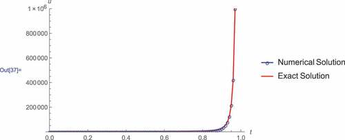We then define $u_m(t)\approx u(x_m,t)$, $\mathbf{u}=[u_1(t),u_2(t),\dots ,u_{M-1}(t){]}^T$, $T$ is the transpose. The problem is now a system of ODEs which is solved by the TDNM. In Figure 1, we show that the numerical method (TDNM) is in good agreement with the exact solution. In Figure 2, we show that the numerical method is in good agreement with the exact solution at $T=1$.

Figure 1. Graphical evidence for Example, 3.6, $M=20,N=80.$ The blow-up in the analytical solution given by (b) is in agreement with that of the approximate solution given by (a). As $t\to 1$, $x\to 1$, $u(1,1)\to \mathrm{\infty }$, which is in agreement with the approximate solution.

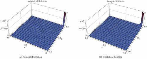
Figure 2. The results provided by the TDNM is in good agreement with the analytical solution. As $t\to 1$, both the analytical and the approximate solutions blow-up.

Specifically, the PDE in 3.6 is computed by letting

(17) $\left\{\begin{array}{c}{f}_{m,n}=\frac{u_{m+1,n}-2u_{m,n}+u_{m-1,n}}{{(\mathrm{\Delta }x)}^2},\\ g_{m,n}=\frac{{u{ }^{\mathrm{\prime }}}_{m+1,n}-2{u{ }^{\mathrm{\prime }}}_{m,n}+{u{ }^{\mathrm{\prime }}}_{m-1,n}}{(\mathrm{\Delta }x)(\mathrm{\Delta }t)},m=1,2,\dots ,M-1,\\ n=0,1,2,\dots ,N.\end{array}\right.$(17)

Example 3.7 We consider the partial differential equation given in (Guo & Yang, 2015).

$u_t=u_{xx}+({\pi }^2-1)u,\hspace{0.17em}x\hspace{0.17em}\text{isin}\hspace{0.17em}[0,1],$

$u(0,t)=0,u(1,t)=0,u(x,0)=sin(\pi x),0\le x\le 1,$

and the exact solution is given by $u(x,t)=e^{-t}sin(\pi x)$.

We obtain the following second-order system after discretizing the time variable $t$ using the second-order finite difference scheme

(18) $\left(\begin{array}{c}\frac{{\mathrm{\partial }}^2{u}_n}{\mathrm{\partial }{x}^2}=-(\frac{u_{n+1}-u_{n-1}}{2\mathrm{\Delta }t})+({\pi }^2-1)u_n,n=1,\dots ,N-1,\\ u(x_m,0)=sin(\pi x_m),\end{array}\right.$(18)

which is written in the form $\mathbf{u}{ }^{\mathrm{\prime }}{ }^{\mathrm{\prime }}\mathbf{=}\mathbf{f}\mathbf{(}\mathbf{x}\mathbf{,}\mathbf{u}\mathbf{)}\mathbf{,}$ subject to the initial conditions $\mathbf{u}(t_0)={\mathbf{u}}_0$, where f($x$, u) = Au+q, A is the matrix arising from the central difference approximations and $q$ is a vector of constants. We then define $u_n(x)\approx u(t_n,x)$, $u=[u_1(x),u_2(x),\dots ,u_{N-1}(x){]}^T$, $T$ is the transpose. In Figure 3, we show that the numerical method is in good agreement with the exact solution at $T=0.1$. 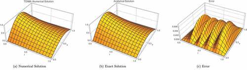We note that this consistency is also observed at $x=1$ where a numerical method could perform poorly (see, (Guo & Yang, 2015)). In Figure 4, we observe that the method performs well when applied to parabolic PDEs as the numerical and exact solutions are in good agreement for all $x$. Hence, the TDNM approximates well the exact solution for the parabolic PDE.

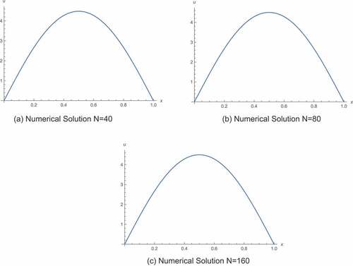
Figure 3. The results provided by the TDNM (M = 10, N = 40) in block unification mode is in good agreement with the analytical solution. We observe that at $x=1$, where a numerical method could perform poorly, the numerical solution is still in good agreement with the analytical solution.

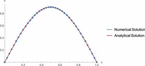
Figure 4. Graphical evidence for Example, 3.7, $M=10,N=40$. The results provided by the TDNM in block unification mode are in good agreement with the exact solution, and the errors are also small, validating the fact the TDNM performs well when applied to parabolic equations.

Specifically, the PDE in 3.7 is computed by letting

(19) $\left\{\begin{array}{c}{f}_{m,n}=-(\frac{u_{m,n+1}-u_{m,n-1}}{2\mathrm{\Delta }t})+({\pi }^2-1)u_{m,n},\\ g_{m,n}=-(\frac{{u{ }^{\mathrm{\prime }}}_{m,n+1}-{u{ }^{\mathrm{\prime }}}_{m,n-1}}{2\mathrm{\Delta }t})+({\pi }^2-1){u{ }^{\mathrm{\prime }}}_{m,n},m=1,2,\dots ,\\ M-1,n=0,1,2,\dots ,N.\end{array}\right.$(19)

Example 3.8 We consider the nonlinear partial differential equation given in (Guo & Yang, 2015).

$u_t=u_{xx}+u^2,\hspace{0.17em}x\hspace{0.17em}\text{isin}\hspace{0.17em}[0,1]$

$u(0,t)=0,u(1,t)=0,u(x,0)=20sin(\pi x),0\le x\le 1$

.

We obtain the following second-order system after discretizing the time variable $t$ using second-order finite difference schemes

(20) $\left(\begin{array}{c}\frac{{\mathrm{\partial }}^2{u}_n}{\mathrm{\partial }{x}^2}=\frac{u_{n+1}-u_{n-1}}{2\mathrm{\Delta }t}-u_n^2,n=1,\dots ,N-1,\\ u(x_m,0)=20sin(\pi x_m),\end{array}\right.$(20)

which is written in the form $\mathbf{u}{ }^{\mathrm{\prime }}{ }^{\mathrm{\prime }}\mathbf{=}\mathbf{f}\mathbf{(}\mathbf{x}\mathbf{,}\mathbf{u}\mathbf{)}\mathbf{,}$ subject to the initial conditions $\mathbf{u}(t_0)={\mathbf{u}}_0$, where f($x$, u) = Au+q, A is the matrix arising from the central difference approximations and $\mathbf{q}$ is a vector of constants. We then define $u_n(x)\approx u(x,t_n)$, $\mathbf{u}=[u_1(x),u_2(x),\dots ,u_{N-1}(x){]}^T$, $T$ is the transpose. The problem is now a system of ordinary differential equations, which is solved by the TDNM. In Figure 5, we show that the TDNM provides results for the reference blow-up time of $T=8.24371\times {10}^{-2}$ for $N=40$, $N=80$, and $N=160$ that are consistent with the results given in (Guo & Yang, 2015). It is observed that the blow-up is located at only one point $x=0.5$ (see, (Guo & Yang, 2015)).

Figure 5. Graphical evidence for Example, 3.8. By considering the reference blow-up time of $T=8.24371\times {10}^{-2}$ for $M=10,N=40,N=80,N=160$, the blow-up time is located only at the point $x=0.5$.

Specifically, the PDE in 3.8 is computed by letting

(21) $\left\{\begin{array}{c}{f}_{m,n}=\frac{u_{m,n+1}-u_{m,n-1}}{2\mathrm{\Delta }t}-u_{m,n}^2,\\ g_{m,n}=-\frac{{u{ }^{\mathrm{\prime }}}_{m,n+1}-{u{ }^{\mathrm{\prime }}}_{m,n-1}}{2\mathrm{\Delta }t}+2u_{m,n}{u{ }^{\mathrm{\prime }}}_{m,n},m=1,2,\dots ,\\ M-1,n=0,1,2,\dots ,N.\end{array}\right.$(21)

4 Conclusions

We have proposed block algorithms based on a TDNM for integrating singular second-order ODEs, including parabolic and hyperbolic PDEs with blow-up solutions. The block algorithms are implemented in a block-by-block mode for IVPs and block unification mode for BVPs. In particular, the algorithms are applied to PDEs by first reducing them into ODEs via the method of lines, whereby the space variable is discretized to yield a system of IVPs and the time variable is discretized to yield a system of BVPs. It is also demonstrated that the implementation of the variable step version of the TDNM, which is generally recommended for challenging IVPs, has no advantage over the block-by-block algorithm. Numerical experiments performed in Section 3 show that the method is accurate and promising. Our future research will be focused on applying multiderivative methods to problems in mathematical biology and mathematical finance.

Disclosure statement

No potential conflict of interest was reported by the author(s).

Additional information

Funding

This research did not receive any specific grant from any funding agencies.

Notes on contributors

S. N. Jator

S. N. Jator is currently a Professor of Mathematics and the Chair of the Department of Mathematics and Statistics, Austin Peay State University, Clarksville, Tennessee, USA. His research interests include Numerical Analysis, Mathematical Biology, Ordinary and Partial Differential Equations, Financial Mathematics, and Predictive Analytics.

N. A. Coleman

N. A. Coleman is currently an Associate Professor of Computer Science at Austin Peay State University, Clarksville, Tennessee, USA. His research interests include Programming Language Semantics, Automata Theory, Formal Methods, Type Theory, and Mathematical Logic.

I. O. Amusan

I. O. Amusan is currently an Assistant Professor in the Department of Mathematics and Statistics at Austin Peay State University, Clarksville, Tennessee, USA. His research interests include Stochastic models, Differential Equations, Numerical Methods, Financial Mathematics, and Actuarial Science.

References

- Bender, C. M., Milton, K. A., Pinsky, S. S., & Simmons, L. M. (1989). A new perturbative approach to nonlinear problems. Journal of Mathematical Physics, 30(7), 1447–11. https://doi.org/10.1063/1.528326
- Budd, C. J., Collins, G. J., & Galaktionov, V. A. (1998). An asymptotic and numerical description of self-similar blow-up in quasilinear parabolic equations. Journal of Computational and Applied Mathematics, 97(1–2), 51–80. https://doi.org/10.1016/S0377-0427(98)00102-2
- Cash, J. R. (1981). Second derivative extended backward differentiation formulas for the numerical integration of stiff systems. SIAM Journal on Numerical Analysis, 18(1), 21–36. https://doi.org/10.1137/0718003
- Cho, C. (2013). On the computation of the numerical blow-up time. Japan Journal of Industrial and Applied Mathematics, 30(2), 331–349. https://doi.org/10.1007/s13160-013-0101-9
- Desaix, M., Anderson, D., & Lisak, M. (2004). Variational approach to the Thomas-Fermi equation. European Journal of Physics, 25(6), 699–705. https://doi.org/10.1088/0143-0807/25/6/001
- Fatunla, S. O. (1991). Block methods for second order IVPs. International Journal of Computer Mathematics, 41(1–2), 55–63. https://doi.org/10.1080/00207169108804026
- Groisman, P. (2006). Totally discrete explicit and semi-implicit Euler methods for a blow-up problem in several space dimensions. Computing, 76(3–4), 325–352. https://doi.org/10.1007/s00607-005-0136-0
- Guo, L., & Yang, Y. (2015). Positivity preserving high-order local discontinuous Galerkin method for parabolic equations with blow-up solutions. Journal of Computational Physics, 289, 181–195. https://doi.org/10.1016/j.jcp.2015.02.041
- Henrici, P. (1962). Discrete variable methods for ODEs. John Wiley.
- Hirota, C., & Ozawa, K. (2006). Numerical method of estimating the blow-up time and rate of the solution of ordinary differential equations-An application to the blow-up problems of partial differential equations. Journal of Computational and Applied Mathematics, 193(2), 614–637. https://doi.org/10.1016/j.cam.2005.04.069
- Jator, S. N. (2012). A continuous two-step method of order 8 with a block extension for y″=f(x. Applied Mathematics and Computation, 219(3), 781–791. https://doi.org/10.1016/j.amc.2012.06.027
- Jator, S. N., Coleman, N., & Katzourakis, N. (2017). A nonlinear second derivative method with a variable step-size based on continued fractions for singular initial value problems. Cogent Mathematics, 4(1), 1335498. https://doi.org/10.1080/23311835.2017.1335498
- Jator, S. N., & Oladejo, H. B. (2017). Block Nyström method for singular differential equations of the Lane-Emden type and problems with highly oscillatory solutions. International Journal of Applied and Computational Mathematics, 3(Suppl S1), 1385–1402. https://doi.org/10.1007/s40819-017-0425-2
- Jator, S. N., Swindle, S., & French, R. (2013). Trigonometrically fitted block Numerov type method for y″=f(x. y,y′), Numerical Algorithms, 62(1), 13–26. https://doi.org/10.1007/s11075-012-9562-1
- Kaur, H., Mittal, R. C., & Mishra, V. (2013). Haar wavelet approximation solutions for the generalized Lane-Emden equations arising from astrophysics. Computer Physics Communications, 184(9), 2169–2177. https://doi.org/10.1016/j.cpc.2013.04.013
- Koch, O., Kofler, P., & Weinmüller, E. B. (2000). The implicit Euler method for the numerical solution of singular initial value problems. Applied Numerical Mathematics, 34(2–3), 231–252. https://doi.org/10.1016/S0168-9274(99)00130-0
- Kumar, M., & Singh, N. (2010). Modified adomian decomposition method and computer implementation for solving singular boundary value problems arising in various physical problems. Computers and Chemical Engineering, 34(11), 1750–1760. https://doi.org/10.1016/j.compchemeng.2010.02.035
- Liao, S. (2003). A new analytic algorithm of Lane-Emden type equation. Applied Mathematics and Computation, 142 (1) , 1–16 https://doi.org/10.1016/S0096-3003(02)00943-8.
- Li, B., & Zhang, Z. (2015). A new approach for numerical simulation of the time-dependent Ginzburg-Landau equations. Journal of Computational Physics, 303, 238–250. https://doi.org/10.1016/j.jcp.2015.09.049
- MacLaurin, J., Chapman, J., Jones, G. W., & Roose, T. (2012). The buckling of capillaries in solid tumours. Proc. R. Soc. A, 468(2148), 4123–4145. https://doi.org/10.1098/rspa.2012.0418
- Ngwane, F. F., & Jator, S. N. (2013). Block hybrid method using trigonometric basis for initial value problems with oscillating solutions. Numerical Algorithms, 63(4), 713–725. https://doi.org/10.1007/s11075-012-9649-8
- Parand, K., Dehghan, M., Rezaei, A. R., & Ghaderi, S. M. (2010). An approximation algorithm for the solution of nonlinear Lane-Emden type equations arising in astrophysics using hermite function collocation method. Computer Physics Communications, 181(6), 1096–1108. https://doi.org/10.1016/j.cpc.2010.02.018
- Rashidinia, J., Mohammadi, R., & Jalilian, R. (2007). The numerical solution of non-linear singular boundary value problems arising in physiology. Applied Mathematics and Computation, 185(1), 360–367. https://doi.org/10.1016/j.amc.2006.06.104
- Russell, R. D., & Shampine, L. F. (1975). Numerical methods for singular boundary value problems. SIAM J. Numer. Anal, 12(1), 13–36. https://doi.org/10.1137/0712002
- Sahlan, M. N., & Hashemizadeh, E. (2015). Wavelet Galerkin method for solving nonlinear singular boundary value problems arising in physiology. Applied Mathematics and Computation, 250, 260–269. https://doi.org/10.1016/j.amc.2014.10.118
- Shiralashetti, S. C., Deshi, A. B., & Mutalik Desai, P. B. (2016). Haar wavelet collocation method for the numerical solution of singular initial value problems. Ain Shams Engineering Journal, 7(2), 663–670. https://doi.org/10.1016/j.asej.2015.06.006
- Sommeijer, B. P. (1993). Explicit high-order Runge-Kutta-Nyström methods for parallel computers. Applied Numerical Mathematics, 13(1–3), 221–240. https://doi.org/10.1016/0168-9274(93)90145-H
- Takayasu, A., Matsue, K., Sasaki, T., Tanaka, K., Mizuguchi, M., & Oishi, S. (2017). Numerical validation of blow-up solutions of ordinary differential equations. Journal of Computational and Applied Mathematics, 314, 10–29. https://doi.org/10.1016/j.cam.2016.10.013
- Wazwaz, A. M. (2001a). A new algorithm for solving differential equations of Lane-Emden type. Applied Mathematics and Computation, 118 (2–3) , 287–310 https://doi.org/10.1016/S0096-3003(99)00223-4.
- Wazwaz, A. M. (2001b). Blow-up for solutions of some linear wave equations with mixed nonlinear boundary conditions. Applied Mathematics and Computation, 123(1), 133–140. https://doi.org/10.1016/S0096-3003(00)00069-2
- Weinmüller, E. B. (1986). On the numerical solution of singular boundary value problems of second order by a difference method. Mathematics of Computation, 46(173), 93–117. https://doi.org/10.1090/S0025-5718-1986-0815834-X
- Xie, L., Zhou, C., & Xu, S. (2016). An effective numerical method to solve a class of nonlinear singular boundary value problems using improved differential transform method. SpringerPlus, 5(1), 1066. https://doi.org/10.1186/s40064-016-2753-9