A novel algorithm for singularly perturbed parabolic differential-difference equations

ABSTRACT

In this study, numerical treatment of singularly perturbed parabolic partial differential-difference equations with small mixed shifts arising in computational neuroscience is presented. Due to the simultaneous presence of a singular perturbation parameter and shifts in the problem applying classical numerical methods to solve such a problem on a uniform mesh are unable to provide oscillation-free results unless they are applied with very fine meshes inside the region. The main objective of the work is to develop and analyze an oscillation-free higher order numerical scheme, which plays a vital role in applications. A uniformly convergent computational scheme is proposed using the implicit Euler method in temporal discretization and the cubic spline in tension method in spatial discretization. The stability and convergence analysis of the method are investigated. The scheme is uniformly convergent with linear order of convergence before Richardson extrapolation and second-order convergent after Richardson extrapolation technique. Three test problems are considered to validate the applicability of the scheme. The efficiency of the proposed scheme is demonstrated by comparing some methods available in the literature. It is observed that the proposed scheme provides more accurate results and higher order of convergence than methods available in the literature.

KEYWORDS:

• Singularly perturbed
• differential-difference equations
• cubic spline in tension method
• implicit Euler method
• uniformly convergent computational scheme

1 Introduction

In the past and recent years, singularly perturbed parabolic differential-difference equations (SPPDDEs) have attracted considerable attention in the scientific community. Such types of equations have prominent roles in many practical models in population dynamics (Kuang, 1993), the study of bistable devices (Derstine et al., 1982), human pupil-light reflex (Andre Longtin, 1988), immune response (Mayer et al., 1995), variational problem in control theory (V.Y. Glizer, 2000; Valery Y. Glizer, 2003), model of colorbluehuman immunodeficiency virus (HIV) infection (Culshaw & Ruan, 2000; Nelson & Perelson, 2002), activation of neuronal variability (Edward et al., 1980; John Wilbur & Rinzel, 1982; Lánskỳ, 1984; Musila & Lánskỳ, 1991; Stein, 1967), the modelling of biological oscillators (Murray, 2007), mathematical ecology (Kot, 2001), models for physiological process (John Mallet-Paret, 1989; Mackey & Glass, 1977), blood cell production (Wazewska-Czyzewska & Lasota, 9176) and so on.

The solution of SPPDDE exhibits sharp boundary and/or interior layers as singular perturbation parameter goes small ($i.e.,\epsilon \to 0$). This multi-scale character makes the numerical treatment of the SPPDDE is very tough to obtain $\epsilon -$ uniform approximate solutions. To overcome this difficulty, various $\epsilon$-uniform numerical methods have been developed using fitted operator and layer-adaptive meshes.

In (Bansal & Kapil, 2017; Bansal & Pratima Rai, 2017; Daba, 2022a, 2021a, 2022b, 2021c, 2021d; Kumar, 2018; Mesfin M. Woldaregay & Duressa, 2019; Nageshwar Rao & Pramod Chakravarthy, 2019; Ramesh & Priyanga, 2019; Woldaregay & Duressa, 2022), authors have suggested various numerical methods based on the fitting approaches to approximate SPPDDE with shift parameter(s). Recently, developing suitable numerical methods for applications of differential equations have received remarkable attention from scholars. For instance, Kostikov and Romanenkov (Kostikov & Romanenkov, 2020) suggested numerical algorithm for solving the optimal control problem for the three-dimensional heat equation. Tene et al (Tene et al., 2021) discussed the analysis of COVID-19 outbreak in Ecuador using the logistic model. Mihajlovic and Zivkovic , 2020 studied sieving extremely wet earth mass by means of oscillatory transporting platform.

Nevertheless, numerical methods to solve SPPDDE in the spatial variable with small and general shift arguments having second order in both directions for the past decade are still few. This drawback initiates us to formulate and analyze almost second-order $\epsilon -$ uniform numerical algorithm in both directions for solving SPPDDE with mixed parameters. The main purpose of this work is to construct and analyze an $\epsilon -$ uniformly convergent numerical method for solving SPPDDE with mixed shifts in the spatial variable. A parameter uniform computational scheme is proposed using the implicit Euler method in time discretization and the cubic spline in tension method in space discretization. The novelty of the presented algorithm, unlike Shishkin and Bakhvalov mesh types, does not require a priori information about the location and width of the boundary layer.

The methods developed by (Bansal & Kapil, 2017; Bansal & Pratima Rai, 2017; Kumar, 2018; Nageshwar Rao & Pramod Chakravarthy, 2019; Ramesh & Priyanga, 2019) for SPPDDE with mixed parameters are based on finite difference method. In comparison with the finite difference methods, spline solution has its own advantages. For instance, once the solution has been computed, the information required for spline interpolation between mesh points is available (Khan et al., 2004). Also, splines are a simpler and more practical way to solve boundary-value problems than finite difference methods (Kumar & Gupta, 2010). This is particularly important when the solution of the boundary-value problem is required at various locations in the interval $[a,b]$. This provides the motivation for our work on using fitted exponential spline method for solving the problem under consideration.

A brief description of the proposed method and its corresponding error analysis are treated in the subsequent sections.

2 The continuous problem

Consider SPPDDE of the form on the domain $\mathrm{\Im }={\mathrm{\Im }}_x\times {\mathrm{\Im }}_t=(0,1)\times (0,T]$ for some fixed number $T>0$:

where $0<\epsilon \ll 1$ is a singular perturbation parameter, $\delta$ is delay and $\eta$ is advance parameter satisfying $\delta ,\eta <\epsilon$. For the existence and uniqueness of the solution, the functions $\omega (x),\varpi (x),\rho (x),\phi (x)$, $\zeta (x,t),{\varsigma }_1(x,t),{\varsigma }_2(x,t)$ and ${\zeta }_0(x)$ are assumed to be sufficiently smooth and bounded with $\varpi (x)+\rho (x)+\phi (x)\ge \theta >0,\mathrm{f}\mathrm{o}\mathrm{r}\mathrm{a}\mathrm{l}\mathrm{l}x\in {\bar{\mathrm{\Im }}}_x$ and for some positive constant $\theta$.

On applying Taylor’s series approximation for $\zeta (x-\delta ,t)$ and $\zeta (x+\eta ,t)$ yields

(2.2) $\zeta (x-\delta ,t)=\zeta (x,t)-\delta \frac{\mathrm{\partial }\zeta (x,t)}{\mathrm{\partial }x}+O({\delta }^2),$(2.2)

(2.3) $\zeta (x+\eta ,t)=\zeta (x,t)+\eta \frac{\mathrm{\partial }\zeta (x,t)}{\mathrm{\partial }x}+O({\eta }^2).$(2.3)

Taking Equation (2.2)(2.2) $\zeta (x-\delta ,t)=\zeta (x,t)-\delta \frac{\mathrm{\partial }\zeta (x,t)}{\mathrm{\partial }x}+O({\delta }^2),$(2.2) and Equation (2.3)(2.3) $\zeta (x+\eta ,t)=\zeta (x,t)+\eta \frac{\mathrm{\partial }\zeta (x,t)}{\mathrm{\partial }x}+O({\eta }^2).$(2.3) into Equation (2.1) gives

(2.4) $\left\{\begin{array}{c}{\text{pound}}_{\epsilon }\zeta (x,t)=\frac{\mathrm{\partial }\zeta \left(x,t\right)}{\mathrm{\partial }t}-{\epsilon }^2\frac{{\mathrm{\partial }}^2\zeta \left(x,t\right)}{\mathrm{\partial }{x}^2}+\xi (x)\frac{\mathrm{\partial }\zeta \left(x,t\right)}{\mathrm{\partial }x}+\nu (x)\zeta (x,t)=\mu (x,t),\\ \zeta (x,0)={\zeta }_0(x),x\in {\bar{\mathrm{\Im }}}_x,\\ \zeta (0,t)={\varsigma }_1(0,t),t\in {\bar{\mathrm{\Im }}}_t,\\ \zeta (1,t)={\varsigma }_2(1,t),t\in {\bar{\mathrm{\Im }}}_t,\end{array}\right.$(2.4)

where $\xi (x)=\omega (x)-\delta \varpi (x)+\eta \phi (x),\nu (x)=\varpi (x)+\rho (x)+$$\phi (x)$. Since $\xi (x)\ge {\xi }^{\ast }>0$ and $\nu (x)\ge {\nu }^{\ast }>0$, the solution of Eq. (2.4(2.4) $\left\{\begin{array}{c}{\text{pound}}_{\epsilon }\zeta (x,t)=\frac{\mathrm{\partial }\zeta \left(x,t\right)}{\mathrm{\partial }t}-{\epsilon }^2\frac{{\mathrm{\partial }}^2\zeta \left(x,t\right)}{\mathrm{\partial }{x}^2}+\xi (x)\frac{\mathrm{\partial }\zeta \left(x,t\right)}{\mathrm{\partial }x}+\nu (x)\zeta (x,t)=\mu (x,t),\\ \zeta (x,0)={\zeta }_0(x),x\in {\bar{\mathrm{\Im }}}_x,\\ \zeta (0,t)={\varsigma }_1(0,t),t\in {\bar{\mathrm{\Im }}}_t,\\ \zeta (1,t)={\varsigma }_2(1,t),t\in {\bar{\mathrm{\Im }}}_t,\end{array}\right.$(2.4) ) reveals boundary layer near $x=1$. For small $\delta$ and $\eta$, Eq. (2.4(2.4) $\left\{\begin{array}{c}{\text{pound}}_{\epsilon }\zeta (x,t)=\frac{\mathrm{\partial }\zeta \left(x,t\right)}{\mathrm{\partial }t}-{\epsilon }^2\frac{{\mathrm{\partial }}^2\zeta \left(x,t\right)}{\mathrm{\partial }{x}^2}+\xi (x)\frac{\mathrm{\partial }\zeta \left(x,t\right)}{\mathrm{\partial }x}+\nu (x)\zeta (x,t)=\mu (x,t),\\ \zeta (x,0)={\zeta }_0(x),x\in {\bar{\mathrm{\Im }}}_x,\\ \zeta (0,t)={\varsigma }_1(0,t),t\in {\bar{\mathrm{\Im }}}_t,\\ \zeta (1,t)={\varsigma }_2(1,t),t\in {\bar{\mathrm{\Im }}}_t,\end{array}\right.$(2.4) ) is gives asymptotically equivalent results to Eq. (2.1).

To secure that the data matches at the two end corners $(0,0)$ and $(1,0)$, we impose compatibility conditions (Ladyzhenskaia et al., 1968) as

(2.5) ${\zeta }_0(0)={\varsigma }_1(0,0),{\zeta }_0(1)={\varsigma }_2(1,0),$(2.5)

and

(2.6) $\left\{\begin{array}{c}\frac{\mathrm{\partial }{\varsigma }_1(0,0)}{\mathrm{\partial }t}-{\epsilon }^2\frac{{\mathrm{\partial }}^2{\zeta }_0(0)}{\mathrm{\partial }{x}^2}+\xi (0)\frac{\mathrm{\partial }{\zeta }_0(0)}{\mathrm{\partial }x}+\nu (0){\zeta }_0(0)=\mu (0,0),\\ \frac{\mathrm{\partial }{\varsigma }_2(1,0)}{\mathrm{\partial }t}-{\epsilon }^2\frac{{\mathrm{\partial }}^2{\zeta }_0(1)}{\mathrm{\partial }{x}^2}+\xi (1)\frac{\mathrm{\partial }{\zeta }_0(1)}{\mathrm{\partial }x}+\nu (1){\zeta }_0(1)=\mu (1,0).\end{array}\right.$(2.6)

The differential operator ${\text{pound}}_{\epsilon }$ in Eq. (2.4(2.4) $\left\{\begin{array}{c}{\text{pound}}_{\epsilon }\zeta (x,t)=\frac{\mathrm{\partial }\zeta \left(x,t\right)}{\mathrm{\partial }t}-{\epsilon }^2\frac{{\mathrm{\partial }}^2\zeta \left(x,t\right)}{\mathrm{\partial }{x}^2}+\xi (x)\frac{\mathrm{\partial }\zeta \left(x,t\right)}{\mathrm{\partial }x}+\nu (x)\zeta (x,t)=\mu (x,t),\\ \zeta (x,0)={\zeta }_0(x),x\in {\bar{\mathrm{\Im }}}_x,\\ \zeta (0,t)={\varsigma }_1(0,t),t\in {\bar{\mathrm{\Im }}}_t,\\ \zeta (1,t)={\varsigma }_2(1,t),t\in {\bar{\mathrm{\Im }}}_t,\end{array}\right.$(2.4) ) satisfies the lemmas.

Lemma 2.1 (Continuous Maximum Principle) If $\mathrm{{\rm Y}}{|}_{\mathrm{\partial }\mathrm{\Im }}\ge 0$ and $\left({\text{pound}}_{\epsilon }\right)\mathrm{{\rm Y}}{|}_{\mathrm{\Im }}\ge 0$, then $\mathrm{{\rm Y}}{|}_{\bar{\mathrm{\Im }}}\ge 0$.

Proof See, (Daba, 2022a)

Lemma 2.2 (Continuous Stability Estimate) The solution $\zeta (x,t)$ of Eq. (2.4(2.4) $\left\{\begin{array}{c}{\text{pound}}_{\epsilon }\zeta (x,t)=\frac{\mathrm{\partial }\zeta \left(x,t\right)}{\mathrm{\partial }t}-{\epsilon }^2\frac{{\mathrm{\partial }}^2\zeta \left(x,t\right)}{\mathrm{\partial }{x}^2}+\xi (x)\frac{\mathrm{\partial }\zeta \left(x,t\right)}{\mathrm{\partial }x}+\nu (x)\zeta (x,t)=\mu (x,t),\\ \zeta (x,0)={\zeta }_0(x),x\in {\bar{\mathrm{\Im }}}_x,\\ \zeta (0,t)={\varsigma }_1(0,t),t\in {\bar{\mathrm{\Im }}}_t,\\ \zeta (1,t)={\varsigma }_2(1,t),t\in {\bar{\mathrm{\Im }}}_t,\end{array}\right.$(2.4) ) is bounded as

$∥\zeta ∥\le {\left({\nu }^{\ast }\right)}^{-1}∥\mu ∥+max\left\{|{\zeta }_0\left(x\right)|,max\left\{|{\varsigma }_1\left(0,t\right)|,|{\varsigma }_2\left(1,t\right)|\right\}\right\},$

Proof See, (Daba, 2022b).

3 Description of the numerical method

We derive the numerical method employing the implicit Euler method and the cubic spline in tension method for the time and space variable derivative, respectively. Consider the partition of the solution domain $[0,1]\times [0,T]$ as

${\mathrm{\Im }}_{\tau }^M=\left\{j\tau ,0<j\le M\right\}\mathrm{a}\mathrm{n}\mathrm{d}{\mathrm{\Im }}_{\mathrm{\ell }}^N=\left\{i\mathrm{\ell },0<i\le N\right\},$

with the temporal and spatial mesh sizes $\tau =T/M$ and $\mathrm{\ell }=1/N,$ respectively. Here, $M$ and $N$ denote the number of nodal points in the temporal and spatial directions.

3.0.1 Temporal semi-discretization

On applying the implicit Euler method on Eq. (2.4(2.4) $\left\{\begin{array}{c}{\text{pound}}_{\epsilon }\zeta (x,t)=\frac{\mathrm{\partial }\zeta \left(x,t\right)}{\mathrm{\partial }t}-{\epsilon }^2\frac{{\mathrm{\partial }}^2\zeta \left(x,t\right)}{\mathrm{\partial }{x}^2}+\xi (x)\frac{\mathrm{\partial }\zeta \left(x,t\right)}{\mathrm{\partial }x}+\nu (x)\zeta (x,t)=\mu (x,t),\\ \zeta (x,0)={\zeta }_0(x),x\in {\bar{\mathrm{\Im }}}_x,\\ \zeta (0,t)={\varsigma }_1(0,t),t\in {\bar{\mathrm{\Im }}}_t,\\ \zeta (1,t)={\varsigma }_2(1,t),t\in {\bar{\mathrm{\Im }}}_t,\end{array}\right.$(2.4) ) in temporal variable yields:

(3.1) $\left\{\begin{array}{c}{\text{pound}}_{\epsilon }^M{\zeta }^{j+1}(x)={\beta }^{j+1}(x),\\ {\zeta }^0(x)={\zeta }_0(x),x\in {\bar{\mathrm{\Im }}}_x,\\ {\zeta }^{j+1}(0{)}^{=}{\phi }_1^{j+1}(0{)}^{,}t\in {\bar{\mathrm{\Im }}}_t,\\ {\zeta }^{j+1}(1)={\phi }_2^{j+1}(1),t\in {\bar{\mathrm{\Im }}}_t,\end{array}\right.$(3.1)

where

${\text{pound}}_{\epsilon }^M=-{\epsilon }^2\frac{d^2{\zeta }^{j+1}(x)}{d{x}^2}+\xi (x)\frac{d{\zeta }^{j+1}(x)}{dx}+\vartheta (x){\zeta }^{j+1}(x),\vartheta (x)=\nu (x)+\frac{1}{\tau },$

${\beta }^{j+1}(x)={\mu }^{j+1}(x)+\frac{{\zeta }^j(x)}{\tau }.$

${\zeta }^{j+1}(x)=\zeta (x,t_{j+1}),{\beta }^{j+1}(x)=\beta (x,t_{j+1})$ and ${\mu }^{j+1}(x)=\mu (x,t_{j+1})$.

Lemma 3.1 (Daba, 2022a). In the solution of Eq. (3.1(3.1) $\left\{\begin{array}{c}{\text{pound}}_{\epsilon }^M{\zeta }^{j+1}(x)={\beta }^{j+1}(x),\\ {\zeta }^0(x)={\zeta }_0(x),x\in {\bar{\mathrm{\Im }}}_x,\\ {\zeta }^{j+1}(0{)}^{=}{\phi }_1^{j+1}(0{)}^{,}t\in {\bar{\mathrm{\Im }}}_t,\\ {\zeta }^{j+1}(1)={\phi }_2^{j+1}(1),t\in {\bar{\mathrm{\Im }}}_t,\end{array}\right.$(3.1) ), the local truncation error estimate $e_{j+1}=\zeta (x,t_{j+1})-{\zeta }^{j+1}(x)$ is bounded by

${∥e_{j+1}∥}_{\mathrm{\infty }}\le C_1{\left(\tau \right)}^2,$

and the global error estimate $E_j=\zeta (x,t_j)-{\zeta }^j(x)$ is given by

${∥E_j∥}_{\mathrm{\infty }}\le C_2(\tau ),\mathrm{\forall }j\le T/\tau ,$

where $C_1,C_2$ are a positive constant independent of $\epsilon$ and $\tau$.

Lemma 3.2 The solution ${\zeta }^{j+1}(x)$ of the Eq. (3.1(3.1) $\left\{\begin{array}{c}{\text{pound}}_{\epsilon }^M{\zeta }^{j+1}(x)={\beta }^{j+1}(x),\\ {\zeta }^0(x)={\zeta }_0(x),x\in {\bar{\mathrm{\Im }}}_x,\\ {\zeta }^{j+1}(0{)}^{=}{\phi }_1^{j+1}(0{)}^{,}t\in {\bar{\mathrm{\Im }}}_t,\\ {\zeta }^{j+1}(1)={\phi }_2^{j+1}(1),t\in {\bar{\mathrm{\Im }}}_t,\end{array}\right.$(3.1) ) is bounded by

(3.2) $∥\frac{{\mathrm{\partial }}^i\zeta (x,t)}{\mathrm{\partial }{x}^n}∥\le C\left(1+{({\epsilon }^2)}^{-n}exp\left(\frac{-({\xi }^{\ast }(1-x))}{{\epsilon }^2}\right)\right),(x,t)\in \bar{\mathrm{\Im }},0\le n\le 4$(3.2)

Proof See, (Kumar, 2018).

3.0.2 Spatial semi-discretization

Here, we approximate the resulting Eq. (3.1(3.1) $\left\{\begin{array}{c}{\text{pound}}_{\epsilon }^M{\zeta }^{j+1}(x)={\beta }^{j+1}(x),\\ {\zeta }^0(x)={\zeta }_0(x),x\in {\bar{\mathrm{\Im }}}_x,\\ {\zeta }^{j+1}(0{)}^{=}{\phi }_1^{j+1}(0{)}^{,}t\in {\bar{\mathrm{\Im }}}_t,\\ {\zeta }^{j+1}(1)={\phi }_2^{j+1}(1),t\in {\bar{\mathrm{\Im }}}_t,\end{array}\right.$(3.1) ) by applying the cubic spline in tension method as described below. A function $S^{j+1}(x,\gamma )\in C^2[0,1]$ which interpolates ${\zeta }^{j+1}(x)$ at the mesh points $x_i$, $i=0,1,\cdots ,N$ depends on a parameter $\gamma >0$ reduces to cubic spline in $[0,1]$ as $\gamma \to 0$ is called parametric cubic spline function. In $[x_i,x_{i+1}]$, the parametric cubic spline function $S^{j+1}(x,\gamma )=S^{j+1}(x)$ satisfies the differential equation (Pramod Chakravarthy et al., 2017):

(3.3) $\begin{array}{cc}\frac{d^2{S}^{j+1}(x)}{d{x}^2}+\gamma S^{j+1}(x)=\left[\frac{d^2{S}^{j+1}(x_i)}{d{x}^2}+\gamma S^{j+1}(x_i)\right]\left(\frac{x_{i+1}-x}{\mathrm{\ell }}\right)& \hspace{0.17em}\\ +\left[\frac{d^2{S}^{j+1}(x_{i+1})}{d{x}^2}+\gamma S^{j+1}(x_{i+1})\right]\left(\frac{x-x_i}{\mathrm{\ell }}\right),& \hspace{0.17em}\end{array}$(3.3)

where $S^{j+1}(x_i)={\zeta }_i^{j+1}$ and $\gamma >0$ is known to be cubic spline in tension.

Solving Eq. (3.3(3.3) $\begin{array}{cc}\frac{d^2{S}^{j+1}(x)}{d{x}^2}+\gamma S^{j+1}(x)=\left[\frac{d^2{S}^{j+1}(x_i)}{d{x}^2}+\gamma S^{j+1}(x_i)\right]\left(\frac{x_{i+1}-x}{\mathrm{\ell }}\right)& \hspace{0.17em}\\ +\left[\frac{d^2{S}^{j+1}(x_{i+1})}{d{x}^2}+\gamma S^{j+1}(x_{i+1})\right]\left(\frac{x-x_i}{\mathrm{\ell }}\right),& \hspace{0.17em}\end{array}$(3.3) ), we obtain

(3.4) $S^{j+1}(x)=A{e}^{\frac{\lambda }{\mathrm{\ell }}x}+B{e}^{\frac{\lambda }{\mathrm{\ell }}x}+\left[\frac{Z_i^{j+1}-\gamma {\zeta }_i^{j+1}}{\gamma }\right]\left(\frac{x-x_{i+1}}{\mathrm{\ell }}\right)+\left[Z_{i+1}^{j+1}-\gamma {\zeta }_{i+1}^{j+1}\right]\left(\frac{x_i-x}{\mathrm{\ell }}\right).$(3.4)

The arbitrary constants $A$ and $B$ can be determined using interpolatory conditions

$S^{j+1}(x_{i+1})={\zeta }_{i+1}^{j+1},S^{j+1}(x_i)={\zeta }_i^{j+1}.$

Putting $\lambda =\mathrm{\ell }{\gamma }^{1/2}$ and $Z_k^{j+1}=\frac{d^2{S}^{j+1}(x_k)}{d{x}^2},k=i,i\pm 1$, we have

(3.5) $\begin{array}{cc}{S}^{j+1}(x)=\frac{{\mathrm{\ell }}^2}{{\lambda }^{2}sinh\lambda }\left[Z_{i+1}^{j+1}sinh\frac{\lambda \left(x-x_i\right)}{\mathrm{\ell }}+Z_i^{j+1}sinh\frac{\lambda \left(x_{i+1}-x\right)}{\mathrm{\ell }}\right]& \hspace{0.17em}\\ -\frac{{\mathrm{\ell }}^2}{{\lambda }^2}\left[\left(\frac{x-x_i}{\mathrm{\ell }}\right)\left(Z_{i+1}^{j+1}-\frac{{\lambda }^2}{\mathrm{\ell }}{\zeta }_{i+1}^{j+1}\right)+\left(\frac{x_{i+1}-x}{\mathrm{\ell }}\right)\left(Z_i^{j+1}-\frac{{\lambda }^2}{\mathrm{\ell }}{\zeta }_i^{j+1}\right)\right].& \hspace{0.17em}\end{array}$(3.5)

Differentiating equation (3.5)(3.5) $\begin{array}{cc}{S}^{j+1}(x)=\frac{{\mathrm{\ell }}^2}{{\lambda }^{2}sinh\lambda }\left[Z_{i+1}^{j+1}sinh\frac{\lambda \left(x-x_i\right)}{\mathrm{\ell }}+Z_i^{j+1}sinh\frac{\lambda \left(x_{i+1}-x\right)}{\mathrm{\ell }}\right]& \hspace{0.17em}\\ -\frac{{\mathrm{\ell }}^2}{{\lambda }^2}\left[\left(\frac{x-x_i}{\mathrm{\ell }}\right)\left(Z_{i+1}^{j+1}-\frac{{\lambda }^2}{\mathrm{\ell }}{\zeta }_{i+1}^{j+1}\right)+\left(\frac{x_{i+1}-x}{\mathrm{\ell }}\right)\left(Z_i^{j+1}-\frac{{\lambda }^2}{\mathrm{\ell }}{\zeta }_i^{j+1}\right)\right].& \hspace{0.17em}\end{array}$(3.5) and taking $x\to x_i$, we obtain

(3.6) $\frac{d{S}^{j+1}(x_i^{+})}{dx}=\frac{{\zeta }_{i+1}^{j+1}-{\zeta }_i^{j+1}}{\mathrm{\ell }}-\frac{\mathrm{\ell }}{{\lambda }^2}\left[\left(1-\frac{\lambda }{sinh}\right)Z_{i+1}^{j+1}-\left(1-\lambda coth\lambda \right)Z_i^{j+1}\right].$(3.6)

Proceeding similarly in the interval $\left(x_{i-1},x_i\right)$, we get

(3.7) $\frac{d{S}^{j+1}(x_i^{-})}{dx}=\frac{{\zeta }_{i+1}^{j+1}-{\zeta }_i^{j+1}}{\mathrm{\ell }}+\frac{\mathrm{\ell }}{{\lambda }^2}\left[-\left(1-\lambda coth\lambda \right)Z_i^{j+1}+\left(1-\frac{\lambda }{sinh\lambda }\right)Z_{i+1}^{j+1}\right].$(3.7)

Equating Eq. (3.6(3.6) $\frac{d{S}^{j+1}(x_i^{+})}{dx}=\frac{{\zeta }_{i+1}^{j+1}-{\zeta }_i^{j+1}}{\mathrm{\ell }}-\frac{\mathrm{\ell }}{{\lambda }^2}\left[\left(1-\frac{\lambda }{sinh}\right)Z_{i+1}^{j+1}-\left(1-\lambda coth\lambda \right)Z_i^{j+1}\right].$(3.6) ) and Eq. (3.7(3.7) $\frac{d{S}^{j+1}(x_i^{-})}{dx}=\frac{{\zeta }_{i+1}^{j+1}-{\zeta }_i^{j+1}}{\mathrm{\ell }}+\frac{\mathrm{\ell }}{{\lambda }^2}\left[-\left(1-\lambda coth\lambda \right)Z_i^{j+1}+\left(1-\frac{\lambda }{sinh\lambda }\right)Z_{i+1}^{j+1}\right].$(3.7) ) at $x_i$, we obtain

(3.8) $\begin{array}{cc}\frac{{\zeta }_i^{j+1}-{\zeta }_{i-1}^{j+1}}{\mathrm{\ell }}+\frac{\mathrm{\ell }}{{\lambda }^2}\left[-\left(1-\lambda coth\lambda \right)Z_i^{j+1}+\left(1-\frac{\lambda }{sinh\lambda }\right)Z_{i-1}^{j+1}\right]& \hspace{0.17em}\\ =\frac{{\zeta }_{i+1}^{j+1}-{\zeta }_i^{j+1}}{\mathrm{\ell }}-\frac{\mathrm{\ell }}{{\lambda }^2}\left[\left(1-\frac{\lambda }{sinh\mathrm{\ell }}\right)Z_{i+1}^{j+1}-\left(1-\lambda coth\lambda \right)Z_i^{j+1}\right].& \hspace{0.17em}\end{array}$(3.8)

Rearranging, we get the following tridiagonal system

(3.9) ${\lambda }_1{Z}_{i+1}^{j+1}+2{\lambda }_2{Z}_i^{j+1}+{\lambda }_1{Z}_{i-1}^{j+1}=\frac{{\zeta }_{i+1}-2{\zeta }_i+{\zeta }_{i-1}}{{\mathrm{\ell }}^2},i=1,2,\cdots N-1,$(3.9)

where ${\lambda }_1=\frac{1}{{\lambda }^2}\left(1-\frac{\lambda }{sinh\lambda }\right),{\lambda }_2=\frac{1}{{\lambda }^2}\left(\lambda coth\lambda -1\right)$.

For the choice of parameters ${\lambda }_1+{\lambda }_2=1/2$ is consistent and suitable for solving the given differential equation.

Now, from Eq. (3.1(3.1) $\left\{\begin{array}{c}{\text{pound}}_{\epsilon }^M{\zeta }^{j+1}(x)={\beta }^{j+1}(x),\\ {\zeta }^0(x)={\zeta }_0(x),x\in {\bar{\mathrm{\Im }}}_x,\\ {\zeta }^{j+1}(0{)}^{=}{\phi }_1^{j+1}(0{)}^{,}t\in {\bar{\mathrm{\Im }}}_t,\\ {\zeta }^{j+1}(1)={\phi }_2^{j+1}(1),t\in {\bar{\mathrm{\Im }}}_t,\end{array}\right.$(3.1) ), we have

(3.10) $\left\{\begin{array}{c}{\epsilon }^2{Z}_{i-1}^{j+1}={\xi }_{i-1}\frac{d{\zeta }_{i-1}^{j+1}}{dx}+{\vartheta }_{i-1}{\zeta }_{i-1}^{j+1}-{\beta }_{i-1}^{j+1},\\ {\epsilon }^2{Z}_i^{j+1}={\xi }_i\frac{d{\zeta }_i^{j+1}}{dx}+{\vartheta }_i{\zeta }_i^{j+1}-{\beta }_i^{j+1},\\ {\epsilon }^2{Z}_{i+1}^{j+1}={\xi }_{i+1}\frac{d{\zeta }_{i+1}^{j+1}}{dx}+{\vartheta }_{i+1}{\zeta }_{i+1}^{j+1}-{\beta }_{i+1}^{j+1},\end{array}\right.$(3.10)

where we approximate $\frac{d{\zeta }_{i+1}^{j+1}}{dx},\frac{d{\zeta }_i^{j+1}}{dx}$ and $\frac{d{\zeta }_{i-1}^{j+1}}{dx}$ as

(3.11) $\left\{\begin{array}{c}\frac{d{\zeta }_{i-1}^{j+1}}{dx}\approx \frac{-{\zeta }_{i+1}^{j+1}+4{\zeta }_i^{j+1}-3{\zeta }_{i-1}^{j+1}}{2\mathrm{\ell }}.\\ \frac{d{\zeta }_i^{j+1}}{dx}\approx \frac{{\zeta }_{i+1}^{j+1}-{\zeta }_{i-1}^{j+1}}{2\mathrm{\ell }},\\ \frac{d{\zeta }_{i+1}^{j+1}}{dx}\approx \frac{3{\zeta }_{i+1}^{j+1}-4{\zeta }_i^{j+1}+{\zeta }_{i-1}^{j+1}}{2\mathrm{\ell }}.\end{array}\right.$(3.11)

Substituting Eq. (3.11(3.11) $\left\{\begin{array}{c}\frac{d{\zeta }_{i-1}^{j+1}}{dx}\approx \frac{-{\zeta }_{i+1}^{j+1}+4{\zeta }_i^{j+1}-3{\zeta }_{i-1}^{j+1}}{2\mathrm{\ell }}.\\ \frac{d{\zeta }_i^{j+1}}{dx}\approx \frac{{\zeta }_{i+1}^{j+1}-{\zeta }_{i-1}^{j+1}}{2\mathrm{\ell }},\\ \frac{d{\zeta }_{i+1}^{j+1}}{dx}\approx \frac{3{\zeta }_{i+1}^{j+1}-4{\zeta }_i^{j+1}+{\zeta }_{i-1}^{j+1}}{2\mathrm{\ell }}.\end{array}\right.$(3.11) ) into (3.10), we have

(3.12) $\left\{\begin{array}{c}{\epsilon }^2{Z}_{i-1}^{j+1}={\xi }_{i-1}\left(\frac{-{\zeta }_{i+1}^{j+1}+4{\zeta }_i^{j+1}-3{\zeta }_{i-1}^{j+1}}{2\mathrm{\ell }}\right)+{\vartheta }_{i-1}{\zeta }_{i-1}^{j+1}-{\beta }_{i-1}^{j+1},\\ {\epsilon }^2{Z}_i^{j+1}={\xi }_i\left(\frac{{\zeta }_{i+1}^{j+1}-{\zeta }_{i-1}^{j+1}}{2\mathrm{\ell }}\right)+{\vartheta }_i{\zeta }_i^{j+1}-{\beta }_i^{j+1},\\ {\epsilon }^2{Z}_{i+1}^{j+1}={\xi }_{i+1}\left(\frac{3{\zeta }_{i+1}^{j+1}-4{\zeta }_i^{j+1}+{\zeta }_{i-1}^{j+1}}{2\mathrm{\ell }}\right)+{\vartheta }_{i+1}{\zeta }_{i+1}^{j+1}-{\beta }_{i+1}^{j+1}.\end{array}\right.$(3.12)

Substituting Eq. (3.12(3.12) $\left\{\begin{array}{c}{\epsilon }^2{Z}_{i-1}^{j+1}={\xi }_{i-1}\left(\frac{-{\zeta }_{i+1}^{j+1}+4{\zeta }_i^{j+1}-3{\zeta }_{i-1}^{j+1}}{2\mathrm{\ell }}\right)+{\vartheta }_{i-1}{\zeta }_{i-1}^{j+1}-{\beta }_{i-1}^{j+1},\\ {\epsilon }^2{Z}_i^{j+1}={\xi }_i\left(\frac{{\zeta }_{i+1}^{j+1}-{\zeta }_{i-1}^{j+1}}{2\mathrm{\ell }}\right)+{\vartheta }_i{\zeta }_i^{j+1}-{\beta }_i^{j+1},\\ {\epsilon }^2{Z}_{i+1}^{j+1}={\xi }_{i+1}\left(\frac{3{\zeta }_{i+1}^{j+1}-4{\zeta }_i^{j+1}+{\zeta }_{i-1}^{j+1}}{2\mathrm{\ell }}\right)+{\vartheta }_{i+1}{\zeta }_{i+1}^{j+1}-{\beta }_{i+1}^{j+1}.\end{array}\right.$(3.12) ) into Eq. (3.9(3.9) ${\lambda }_1{Z}_{i+1}^{j+1}+2{\lambda }_2{Z}_i^{j+1}+{\lambda }_1{Z}_{i-1}^{j+1}=\frac{{\zeta }_{i+1}-2{\zeta }_i+{\zeta }_{i-1}}{{\mathrm{\ell }}^2},i=1,2,\cdots N-1,$(3.9) ) and rearranging, we get

(3.13) $\begin{array}{rl}& {\epsilon }^2\left(\frac{{\zeta }_{i-1}^{j+1}-2{\zeta }_i^{j+1}+{\zeta }_{i+1}^{j+1}}{{\mathrm{\ell }}^2}\right)=\left(\frac{-3{\lambda }_1{\xi }_{i-1}}{2\mathrm{\ell }}+{\lambda }_1{\vartheta }_{i-1}-\frac{{\lambda }_2{\xi }_i}{\mathrm{\ell }}+\frac{{\lambda }_1{\xi }_{i+1}}{2\mathrm{\ell }}\right){\zeta }_{i-1}^{j+1}+\\ & \left(\frac{-2{\lambda }_1{\xi }_{i-1}}{\mathrm{\ell }}+2{\lambda }_2{\vartheta }_i+\frac{2{\lambda }_1{\xi }_{i+1}}{\mathrm{\ell }}\right){\zeta }_i^{j+1}+\left(\frac{-{\lambda }_1{\xi }_{i-1}}{2\mathrm{\ell }}+\frac{{\lambda }_2{\xi }_i}{\mathrm{\ell }}+\frac{3{\lambda }_1{\xi }_{i+1}}{2\mathrm{\ell }}+{\lambda }_1{\vartheta }_{i+1}\right){\zeta }_{i+1}^{j+1}\\ & -{\lambda }_1{\beta }_{i-1}^{j+1}-2{\lambda }_2{\beta }_i^{j+1}-{\lambda }_1{\beta }_{i+1}^{j+1}.\end{array}$(3.13)

To handle the effect of $\epsilon$ a constant fitting factor $\sigma (\rho )$ is multiplied on the term containing $\epsilon$ as

(3.14) $\begin{array}{rl}& \sigma (\rho ){\epsilon }^2\left(\frac{{\zeta }_{i-1}^{j+1}-2{\zeta }_i^{j+1}+{\zeta }_{i+1}}{{\mathrm{\ell }}^2}\right)=\left(\frac{-3{\lambda }_1{\xi }_{i-1}}{2\mathrm{\ell }}+{\lambda }_1{\vartheta }_{i-1}-\frac{{\lambda }_2{\xi }_i}{\mathrm{\ell }}+\frac{{\lambda }_1{\xi }_{i+1}}{2\mathrm{\ell }}\right){\zeta }_{i-1}^{j+1}+\\ & \left(\frac{-2{\lambda }_1{\xi }_{i-1}}{\mathrm{\ell }}+2{\lambda }_2{\vartheta }_i+\frac{2{\lambda }_1{\xi }_{i+1}}{\mathrm{\ell }}\right){\zeta }_i^{j+1}+\left(\frac{-{\lambda }_1{\xi }_{i-1}}{2\mathrm{\ell }}+\frac{{\lambda }_2{\xi }_i}{\mathrm{\ell }}+\frac{3{\lambda }_1{\xi }_{i+1}}{2\mathrm{\ell }}+{\lambda }_1{\vartheta }_{i+1}\right){\zeta }_{i+1}^{j+1}\\ & -{\lambda }_1{\beta }_{i-1}^{j+1}-2{\lambda }_2{\beta }_i^{j+1}-{\lambda }_1{\beta }_{i+1}^{j+1}.\end{array}$(3.14)

Multiplying Eq. (3.14) by $\mathrm{\ell }$ and taking the limit as $\mathrm{\ell }\to 0$, we get

(3.15) $\underset{h\to 0}{lim}\sigma (\rho ){\epsilon }^2\left(\frac{{\zeta }_{i-1}^{j+1}-2{\zeta }_i^{j+1}+{\zeta }_{i+1}^{j+1}}{\mathrm{\ell }}\right)-\frac{\xi (0)}{2}\left({\zeta }_{i+1}^{j+1}-{\zeta }_{i-1}^{j+1}\right)=0.$(3.15)

For problems with a layer at the right end of the interval, from the theory of singular perturbations, the solution of Eq. (3.1(3.1) $\left\{\begin{array}{c}{\text{pound}}_{\epsilon }^M{\zeta }^{j+1}(x)={\beta }^{j+1}(x),\\ {\zeta }^0(x)={\zeta }_0(x),x\in {\bar{\mathrm{\Im }}}_x,\\ {\zeta }^{j+1}(0{)}^{=}{\phi }_1^{j+1}(0{)}^{,}t\in {\bar{\mathrm{\Im }}}_t,\\ {\zeta }^{j+1}(1)={\phi }_2^{j+1}(1),t\in {\bar{\mathrm{\Im }}}_t,\end{array}\right.$(3.1) ) is of the form (O’Malley, 1991)

(3.16) ${\zeta }^{j+1}(x)\approx {\zeta }_0^{j+1}(x)+\frac{\xi (1)}{\xi (x)}\left({\varsigma }^{j+1}(2)-{\zeta }_0^{j+1}(x)\right)exp\left(-\xi (x)\frac{1-x}{{\epsilon }^2}\right)+O(\epsilon ),$(3.16)

where ${\zeta }_0^{j+1}(x)$ is the solution of the reduced problem

$\xi (x)\frac{d{\zeta }_0^{j+1}(x)}{dx}+\vartheta (x){\zeta }_0^{j+1}(x)={\beta }^{j+1}(x)\mathrm{w}\mathrm{i}\mathrm{t}\mathrm{h}{\varsigma }^{j+1}(1)={\varsigma }^{j+1}(2).$

Taking Taylor’s series expansion for $\xi (x)$ about the point $x=1$ and restricting to their first terms, Eq. (3.16(3.16) ${\zeta }^{j+1}(x)\approx {\zeta }_0^{j+1}(x)+\frac{\xi (1)}{\xi (x)}\left({\varsigma }^{j+1}(2)-{\zeta }_0^{j+1}(x)\right)exp\left(-\xi (x)\frac{1-x}{{\epsilon }^2}\right)+O(\epsilon ),$(3.16) ) becomes

(3.17) ${\zeta }^{j+1}(x)\approx {\zeta }_0^{j+1}(x)+\left({\varsigma }^{j+1}(2)-{\zeta }_0^{j+1}(1)\right)exp\left(-\xi (1)\left(\frac{1-x}{{\epsilon }^2}\right)\right)+O(\epsilon ).$(3.17)

Now, from the Eq. (3.17(3.17) ${\zeta }^{j+1}(x)\approx {\zeta }_0^{j+1}(x)+\left({\varsigma }^{j+1}(2)-{\zeta }_0^{j+1}(1)\right)exp\left(-\xi (1)\left(\frac{1-x}{{\epsilon }^2}\right)\right)+O(\epsilon ).$(3.17) ), we have

where $\rho =\frac{\mathrm{\ell }}{{\epsilon }^2}$. Plugging the above equations into Eq. (3.15(3.15) $\underset{h\to 0}{lim}\sigma (\rho ){\epsilon }^2\left(\frac{{\zeta }_{i-1}^{j+1}-2{\zeta }_i^{j+1}+{\zeta }_{i+1}^{j+1}}{\mathrm{\ell }}\right)-\frac{\xi (0)}{2}\left({\zeta }_{i+1}^{j+1}-{\zeta }_{i-1}^{j+1}\right)=0.$(3.15) ) gives the required fitting factor

(3.18) $\sigma \left(\rho \right)=\frac{\xi (0)\rho }{2}coth\left(\frac{\xi (1)\rho }{2}\right).$(3.18)

Finally, from Equation (3.14)(3.14) $\begin{array}{rl}& \sigma (\rho ){\epsilon }^2\left(\frac{{\zeta }_{i-1}^{j+1}-2{\zeta }_i^{j+1}+{\zeta }_{i+1}}{{\mathrm{\ell }}^2}\right)=\left(\frac{-3{\lambda }_1{\xi }_{i-1}}{2\mathrm{\ell }}+{\lambda }_1{\vartheta }_{i-1}-\frac{{\lambda }_2{\xi }_i}{\mathrm{\ell }}+\frac{{\lambda }_1{\xi }_{i+1}}{2\mathrm{\ell }}\right){\zeta }_{i-1}^{j+1}+\\ & \left(\frac{-2{\lambda }_1{\xi }_{i-1}}{\mathrm{\ell }}+2{\lambda }_2{\vartheta }_i+\frac{2{\lambda }_1{\xi }_{i+1}}{\mathrm{\ell }}\right){\zeta }_i^{j+1}+\left(\frac{-{\lambda }_1{\xi }_{i-1}}{2\mathrm{\ell }}+\frac{{\lambda }_2{\xi }_i}{\mathrm{\ell }}+\frac{3{\lambda }_1{\xi }_{i+1}}{2\mathrm{\ell }}+{\lambda }_1{\vartheta }_{i+1}\right){\zeta }_{i+1}^{j+1}\\ & -{\lambda }_1{\beta }_{i-1}^{j+1}-2{\lambda }_2{\beta }_i^{j+1}-{\lambda }_1{\beta }_{i+1}^{j+1}.\end{array}$(3.14) and (3.18(3.18) $\sigma \left(\rho \right)=\frac{\xi (0)\rho }{2}coth\left(\frac{\xi (1)\rho }{2}\right).$(3.18) ), we get

(3.19) ${\text{pound}}_{\epsilon }^{N,M}{\zeta }_i^{j+1}=H_i^{j+1},i=1,2,\cdots ,N-1,$(3.19)

where

$\left\{\begin{array}{c}{\text{pound}}_{\epsilon }^{N,M}{\zeta }_i^{j+1}={\chi }_i^{-}{\zeta }_{i-1}^{j+1}+{\chi }_i^c{\zeta }_i^{j+1}+{\chi }_i^{+}{\zeta }_{i+1}^{j+1}\\ {\chi }_i^{-}=-\frac{\sigma (\rho ){\epsilon }^2}{{\mathrm{\ell }}^2}-\frac{3{\lambda }_1{\xi }_{i-1}}{2h}-\frac{{\lambda }_2{\xi }_i}{\mathrm{\ell }}+\frac{{\lambda }_1{\xi }_{i+1}}{2h}+{\lambda }_1{\vartheta }_{i-1},\\ {\chi }_i^c=\frac{2\sigma (\rho ){\epsilon }^2}{{\mathrm{\ell }}^2}-\frac{2{\lambda }_1{\xi }_{i-1}}{\mathrm{\ell }}+2{\lambda }_2{\vartheta }_i+\frac{2{\lambda }_1{\xi }_{i+1}}{\mathrm{\ell }},\\ {\chi }_i^{+}=-\frac{\sigma (\rho ){\epsilon }^2}{{\mathrm{\ell }}^2}-\frac{{\lambda }_1{\xi }_{i-1}}{2\mathrm{\ell }}+\frac{{\lambda }_2{\xi }_i}{\mathrm{\ell }}+\frac{3{\lambda }_1{\xi }_{i+1}}{2\mathrm{\ell }}+{\lambda }_1{\vartheta }_{i+1},\\ H_i^{j+1}={\lambda }_1{\beta }_{i-1}^{j+1}+2{\lambda }_2{\beta }_i^{j+1}+{\lambda }_1{\beta }_{i+1}^{j+1}.\end{array}\right.$

For sufficiently small $\mathrm{\ell }$, the above matrix is non-singular and $|{\chi }_i^c|\ge |{\chi }_i^{-}|+|{\chi }_i^{+}|$ ($i.e.,$ the matrix are diagonally dominant). Hence, by (Nichols, 1989), the matrix $\chi$ is M-matrix and have an inverse. Therefore, the system of equations can be solved by matrix inverse.

4 Convergence analysis

Lemma 4.1 (Discrete Maximum Principle) If the discrete function ${\mathrm{{\rm Y}}}_i^{j+1}$ satisfies ${\mathrm{{\rm Y}}}_i^{j+1}{|}_{\mathrm{\partial }\mathrm{\Im }}\ge 0$ and $\left({\text{pound}}_{\epsilon }^{N,M}\right){\mathrm{{\rm Y}}}_i^{j+1}{|}_{\mathrm{\Im }}\ge 0$, then ${\mathrm{{\rm Y}}}_i^{j+1}{|}_{\bar{\mathrm{\Im }}}\ge 0$.

Proof Proof follows from the Like quarrels as secondhand in Lemma 2.1.

Lemma 4.2 (Discrete Uniform Stability) The solution ${\zeta }_i^{j+1}$ of the Eq. (3.19(3.19) ${\text{pound}}_{\epsilon }^{N,M}{\zeta }_i^{j+1}=H_i^{j+1},i=1,2,\cdots ,N-1,$(3.19) ) at $(j+1)th$ time level and $\mathrm{\Gamma }=\underset{0\le i\le N}{min}\left\{{\vartheta }_i\right\}$, where $\mathrm{\Gamma }$ is some positive constant is bounded as

$∥{\zeta }_i^{j+1}∥\le \frac{∥{\text{pound}}_{\epsilon }^{N,M}{\zeta }_i^{j+1}∥}{\mathrm{\Gamma }}+max\left\{|{\zeta }_0^{j+1}|,|{\zeta }_N^{j+1}|\right\}.$

Proof Let define barrier functions ${\left({\mathrm{\Theta }}_{\mathrm{i}}^{\mathrm{j}+1}\right)}^{\pm }$ as ${\left({\mathrm{\Theta }}_{\mathrm{i}}^{\mathrm{j}+1}\right)}^{\pm }=\mathrm{\Xi }\pm {\zeta }_i^{j+1},$where $\mathrm{\Xi }=\frac{∥{\text{pound}}_{\epsilon }^{N,M}{\zeta }_i^{j+1}∥}{\mathrm{\Gamma }}+max\left\{|{\zeta }_0^{j+1}|,|{\zeta }_N^{j+1}|\right\}$. On the boundary points, we obtain

${\Theta }_0^{j+1}\pm =\Xi \pm {\zeta }_0^{j+1}=\frac{\Vert {\pounds }_{\epsilon }^{N,M}{\zeta }_i^{j+1}\Vert }{\Gamma }+\max \left\{\left|{\zeta }_0^{j+1}\right|,\left|{\zeta }_N^{j+1}\right|\right\}\pm {\varsigma }_1^{j+1}(0)\ge 0,$

${\left({\mathrm{\Theta }}_{\mathrm{N}}^{\mathrm{j}+1}\right)}^{\pm }=\mathrm{\Xi }\pm {\zeta }_N^{j+1}=\frac{∥{\text{pound}}_{\epsilon }^{N,M}{\zeta }_i^{j+1}∥}{\mathrm{\Gamma }}\text{break}+max\left\{|{\zeta }_0^{j+1}|,|{\zeta }_N^{j+1}|\right\}\pm {\varsigma }_2^{j+1}(N)\ge 0.$

Now, on the discretized spatial domain ${\mathrm{\Im }}_{\mathrm{\ell }}^N$, we have

$\begin{array}{rl}& {\text{pound}}_{\epsilon }^{N,M}{\left({\mathrm{\Theta }}_{\mathrm{i}}^{\mathrm{j}+1}\right)}^{\pm }={\text{pound}}_{\epsilon }^{N,M}\left(\mathrm{\Xi }\pm {\zeta }_i^{j+1}\right)\\ & =\left(-\frac{\sigma (\rho ){\epsilon }^2}{{\mathrm{\ell }}^2}-\frac{3{\lambda }_1{\xi }_{i-1}}{2\mathrm{\ell }}-\frac{{\lambda }_2{\xi }_i}{\mathrm{\ell }}+\frac{{\lambda }_1{\xi }_{i+1}}{2\mathrm{\ell }}+{\lambda }_1{\vartheta }_{i-1}\right)\left(\mathrm{\Xi }\pm {\zeta }_{i-1}^{j+1}\right)\\ & +\left(\frac{2\sigma (\rho ){\epsilon }^2}{{\mathrm{\ell }}^2}-\frac{2{\lambda }_1{\xi }_{i-1}}{\mathrm{\ell }}+2{\lambda }_2{\vartheta }_i+\frac{2{\lambda }_1{\xi }_{i+1}}{\mathrm{\ell }}\right)\left(\mathrm{\Xi }\pm {\zeta }_i^{j+1}\right)\\ & +\left(-\frac{\sigma (\rho ){\epsilon }^2}{{\mathrm{\ell }}^2}-\frac{{\lambda }_1{\xi }_{i-1}}{2\mathrm{\ell }}+\frac{{\lambda }_2{\xi }_i}{\mathrm{\ell }}+\frac{3{\lambda }_1{\xi }_{i+1}}{2\mathrm{\ell }}+{\lambda }_1{\vartheta }_{i+1}\right)\left(\mathrm{\Xi }\pm {\zeta }_{i+1}^{j+1}\right),\end{array}$

$\begin{array}{rl}& =\pm \left(-\frac{\sigma (\rho ){\epsilon }^2}{{\mathrm{\ell }}^2}-\frac{3{\lambda }_1{\xi }_{i-1}}{2\mathrm{\ell }}-\frac{{\lambda }_2{\xi }_i}{\mathrm{\ell }}+\frac{{\lambda }_1{\xi }_{i+1}}{2\mathrm{\ell }}+{\lambda }_1{\vartheta }_{i-1}\right){\zeta }_{i-1}^{j+1}\\ & \pm \left(\frac{2\sigma (\rho ){\epsilon }^2}{{\mathrm{\ell }}^2}-\frac{2{\lambda }_1{\xi }_{i-1}}{\mathrm{\ell }}+\frac{2{\lambda }_1{\xi }_{i+1}}{\mathrm{\ell }}+2{\lambda }_2{\vartheta }_i\right){\zeta }_i^{j+1}\\ & \pm \left(-\frac{\sigma (\rho ){\epsilon }^2}{{\mathrm{\ell }}^2}-\frac{{\lambda }_1{\xi }_{i-1}}{2\mathrm{\ell }}+\frac{{\lambda }_2{\xi }_i}{\mathrm{\ell }}+\frac{3{\lambda }_1{\xi }_{i+1}}{2\mathrm{\ell }}+{\lambda }_1{\vartheta }_{i+1}\right){\zeta }_{i+1}^{j+1}\\ & +\left({\lambda }_1{\vartheta }_{i-1}+2{\lambda }_2{\vartheta }_i+{\lambda }_1{\vartheta }_{i+1}\right)\mathrm{\Xi },,\\ & \pm \left({\lambda }_1{\beta }_{i-1}^{j+1}+2{\lambda }_2{\beta }_i^{j+1}+{\lambda }_1{\beta }_{i+1}^{j+1}\right)+\left({\lambda }_1{\vartheta }_{i-1}+2{\lambda }_2{\vartheta }_i+{\lambda }_1{\vartheta }_{i+1}\right)\mathrm{\Xi },\\ & =\left({\lambda }_1{\vartheta }_{i-1}+2{\lambda }_2{\vartheta }_i+{\lambda }_1{\vartheta }_{i+1}\right)\left(\frac{∥{\text{pound}}_{\epsilon }^{N,M}{\zeta }_i^{j+1}∥}{\mathrm{\Gamma }}+max\left\{|{\zeta }_0^{j+1}|,|{\zeta }_N^{j+1}|\right\}\right)\\ & \mp ({\lambda }_1{\beta }_{i-1}^{j+1}+2{\lambda }_2{\beta }_i^{j+1}+{\lambda }_1{\beta }_{i+1}^{j+1})\\ & \ge 0,\mathrm{s}\mathrm{i}\mathrm{n}\mathrm{c}\mathrm{e}\vartheta (x_i)\ge \mathrm{\Gamma }>0.\end{array}$

On applying Lemma 4.1, we obtain ${\left({\mathrm{\Theta }}_{\mathrm{i}}^{\mathrm{j}+1}\right)}^{\pm }\ge 0,\mathrm{f}\mathrm{o}\mathrm{r}\mathrm{a}\mathrm{l}\mathrm{l}{x}_i\in {\bar{\mathrm{\Im }}}_{\mathrm{\ell }}^N$. Hence, the desired bound is obtained.

Lemma 4.3 The local truncation error in space discretization of the discrete problem (3.19) is given as

$\underset{i,j}{max}|{\zeta }^{j+1}(x_i)-{\zeta }_i^{j+1}|\le C{\mathrm{\ell }}^2,$

where $C$ is a constant independent of $\epsilon$ and $\mathrm{\ell }$.

Proof From the truncation error of Eq. (3.11(3.11) $\left\{\begin{array}{c}\frac{d{\zeta }_{i-1}^{j+1}}{dx}\approx \frac{-{\zeta }_{i+1}^{j+1}+4{\zeta }_i^{j+1}-3{\zeta }_{i-1}^{j+1}}{2\mathrm{\ell }}.\\ \frac{d{\zeta }_i^{j+1}}{dx}\approx \frac{{\zeta }_{i+1}^{j+1}-{\zeta }_{i-1}^{j+1}}{2\mathrm{\ell }},\\ \frac{d{\zeta }_{i+1}^{j+1}}{dx}\approx \frac{3{\zeta }_{i+1}^{j+1}-4{\zeta }_i^{j+1}+{\zeta }_{i-1}^{j+1}}{2\mathrm{\ell }}.\end{array}\right.$(3.11) ), we have

(4.1) $\left\{\begin{array}{c}{e{ }^{\mathrm{\prime }}}_{i+1}=\frac{d{\zeta }^{j+1}(x_{i+1})}{dx}-\frac{d{\zeta }_{i+1}^{j+1}}{dx}=\frac{{\mathrm{\ell }}^2}{3}\frac{d^3{\zeta }^{j+1}(x_i)}{d{x}^3}+\frac{{\mathrm{\ell }}^3}{12}\frac{d^4{\zeta }^{j+1}(x_i)}{d{x}^4}+\frac{{\mathrm{\ell }}^4}{30}\frac{d^5{\zeta }^{j+1}({\xi }_i)}{d{x}^5},\\ {e{ }^{\mathrm{\prime }}}_i=\frac{d{\zeta }^{j+1}(x_i)}{dx}-\frac{d{\zeta }_i^{j+1}}{dx}=-\frac{{\mathrm{\ell }}^2}{6}\frac{d^3{\zeta }^{j+1}(x_i)}{d{x}^3}-\frac{{\mathrm{\ell }}^4}{120}\frac{d^5{\zeta }^{j+1}({\xi }_i)}{d{x}^5},\\ {e{ }^{\mathrm{\prime }}}_{i+1}=\frac{d{\zeta }^{j+1}(x_{i+1})}{dx}-\frac{d{\zeta }_{i+1}^{j+1}}{dx}=\frac{{\mathrm{\ell }}^2}{3}\frac{d^3{\zeta }^{j+1}(x_i)}{d{x}^3}+\frac{{\mathrm{\ell }}^3}{12}\frac{d^4{\zeta }^{j+1}(x_i)}{d{x}^4}+\frac{{\mathrm{\ell }}^4}{30}\frac{d^5{\zeta }^{j+1}({\xi }_i)}{d{x}^5},\end{array}\right.$(4.1)

where $x_{i-1}<\psi <x_{i+1}$. Substituting

$\sigma {\epsilon }^2{Z}_k^{j+1}={\xi }_k\frac{d{\zeta }_k^{j+1}}{dx}+{\vartheta }_k{\zeta }_k^{j+1}-{\beta }_k^{j+1},k=i,i\pm 1$

into Eq. (3.9(3.9) ${\lambda }_1{Z}_{i+1}^{j+1}+2{\lambda }_2{Z}_i^{j+1}+{\lambda }_1{Z}_{i-1}^{j+1}=\frac{{\zeta }_{i+1}-2{\zeta }_i+{\zeta }_{i-1}}{{\mathrm{\ell }}^2},i=1,2,\cdots N-1,$(3.9) ), we get

(4.2) $\begin{array}{rl}& \sigma {\epsilon }^2\left({\zeta }_{i-1}^{j+1}-2{\zeta }_i^{j+1}+{\zeta }_{i+1}^{j+1}\right)={\mathrm{\ell }}^2{\lambda }_1\left({\xi }_{i-1}\frac{d{\zeta }_{i-1}^{j+1}}{dx}+{\vartheta }_{i-1}{\zeta }_{i-1}^{j+1}-{\beta }_{i-1}^{j+1}\right)\\ & +2{\mathrm{\ell }}^2{\lambda }_2\left({\xi }_i\frac{d{\zeta }_i^{j+1}}{dx}+{\vartheta }_i{\zeta }_i^{j+1}-{\beta }_i^{j+1}\right)\\ & +{\mathrm{\ell }}^2{\lambda }_1\left({\xi }_{i+1}\frac{d{\zeta }_{i+1}^{j+1}}{dx}+{\vartheta }_{i+1}{\zeta }_{i+1}^{j+1}-{\beta }_{i+1}^{j+1}\right).\end{array}$(4.2)

Considering the corresponding exact solution to Eq. (4.2(4.2) $\begin{array}{rl}& \sigma {\epsilon }^2\left({\zeta }_{i-1}^{j+1}-2{\zeta }_i^{j+1}+{\zeta }_{i+1}^{j+1}\right)={\mathrm{\ell }}^2{\lambda }_1\left({\xi }_{i-1}\frac{d{\zeta }_{i-1}^{j+1}}{dx}+{\vartheta }_{i-1}{\zeta }_{i-1}^{j+1}-{\beta }_{i-1}^{j+1}\right)\\ & +2{\mathrm{\ell }}^2{\lambda }_2\left({\xi }_i\frac{d{\zeta }_i^{j+1}}{dx}+{\vartheta }_i{\zeta }_i^{j+1}-{\beta }_i^{j+1}\right)\\ & +{\mathrm{\ell }}^2{\lambda }_1\left({\xi }_{i+1}\frac{d{\zeta }_{i+1}^{j+1}}{dx}+{\vartheta }_{i+1}{\zeta }_{i+1}^{j+1}-{\beta }_{i+1}^{j+1}\right).\end{array}$(4.2) ), we have

Subtracting Eq. (4.2(4.2) $\begin{array}{rl}& \sigma {\epsilon }^2\left({\zeta }_{i-1}^{j+1}-2{\zeta }_i^{j+1}+{\zeta }_{i+1}^{j+1}\right)={\mathrm{\ell }}^2{\lambda }_1\left({\xi }_{i-1}\frac{d{\zeta }_{i-1}^{j+1}}{dx}+{\vartheta }_{i-1}{\zeta }_{i-1}^{j+1}-{\beta }_{i-1}^{j+1}\right)\\ & +2{\mathrm{\ell }}^2{\lambda }_2\left({\xi }_i\frac{d{\zeta }_i^{j+1}}{dx}+{\vartheta }_i{\zeta }_i^{j+1}-{\beta }_i^{j+1}\right)\\ & +{\mathrm{\ell }}^2{\lambda }_1\left({\xi }_{i+1}\frac{d{\zeta }_{i+1}^{j+1}}{dx}+{\vartheta }_{i+1}{\zeta }_{i+1}^{j+1}-{\beta }_{i+1}^{j+1}\right).\end{array}$(4.2) ) from Eq. (4.3(4.2) $\begin{array}{rl}& \sigma {\epsilon }^2\left({\zeta }_{i-1}^{j+1}-2{\zeta }_i^{j+1}+{\zeta }_{i+1}^{j+1}\right)={\mathrm{\ell }}^2{\lambda }_1\left({\xi }_{i-1}\frac{d{\zeta }_{i-1}^{j+1}}{dx}+{\vartheta }_{i-1}{\zeta }_{i-1}^{j+1}-{\beta }_{i-1}^{j+1}\right)\\ & +2{\mathrm{\ell }}^2{\lambda }_2\left({\xi }_i\frac{d{\zeta }_i^{j+1}}{dx}+{\vartheta }_i{\zeta }_i^{j+1}-{\beta }_i^{j+1}\right)\\ & +{\mathrm{\ell }}^2{\lambda }_1\left({\xi }_{i+1}\frac{d{\zeta }_{i+1}^{j+1}}{dx}+{\vartheta }_{i+1}{\zeta }_{i+1}^{j+1}-{\beta }_{i+1}^{j+1}\right).\end{array}$(4.2) ) and denoting $e_k={\zeta }^{j+1}(x_k)-{\zeta }_k^{j+1}$ for $k=i,i\pm 1$ we arrive at

(4.4) $\begin{array}{rl}& \left(\sigma {\epsilon }^2-{\mathrm{\ell }}^2{\lambda }_1{\vartheta }_{i-1}\right)e_{i-1}+\left(-2\sigma {\epsilon }^2-2{\mathrm{\ell }}^2{\lambda }_2{\vartheta }_i\right)e_i+\left(\sigma {\epsilon }^2-{\mathrm{\ell }}^2{\lambda }_1{\vartheta }_{i+1}\right)e_{i+1}\\ & ={\mathrm{\ell }}^2\left({\lambda }_1{\xi }_{i-1}{e{ }^{\mathrm{\prime }}}_{i-1}+2{\lambda }_2{\xi }_i{e{ }^{\mathrm{\prime }}}_i+{\lambda }_1{\xi }_{i+1}{e{ }^{\mathrm{\prime }}}_{i+1}.\right)\end{array}$(4.4)

Inserting Eq. (4.1(4.1) $\left\{\begin{array}{c}{e{ }^{\mathrm{\prime }}}_{i+1}=\frac{d{\zeta }^{j+1}(x_{i+1})}{dx}-\frac{d{\zeta }_{i+1}^{j+1}}{dx}=\frac{{\mathrm{\ell }}^2}{3}\frac{d^3{\zeta }^{j+1}(x_i)}{d{x}^3}+\frac{{\mathrm{\ell }}^3}{12}\frac{d^4{\zeta }^{j+1}(x_i)}{d{x}^4}+\frac{{\mathrm{\ell }}^4}{30}\frac{d^5{\zeta }^{j+1}({\xi }_i)}{d{x}^5},\\ {e{ }^{\mathrm{\prime }}}_i=\frac{d{\zeta }^{j+1}(x_i)}{dx}-\frac{d{\zeta }_i^{j+1}}{dx}=-\frac{{\mathrm{\ell }}^2}{6}\frac{d^3{\zeta }^{j+1}(x_i)}{d{x}^3}-\frac{{\mathrm{\ell }}^4}{120}\frac{d^5{\zeta }^{j+1}({\xi }_i)}{d{x}^5},\\ {e{ }^{\mathrm{\prime }}}_{i+1}=\frac{d{\zeta }^{j+1}(x_{i+1})}{dx}-\frac{d{\zeta }_{i+1}^{j+1}}{dx}=\frac{{\mathrm{\ell }}^2}{3}\frac{d^3{\zeta }^{j+1}(x_i)}{d{x}^3}+\frac{{\mathrm{\ell }}^3}{12}\frac{d^4{\zeta }^{j+1}(x_i)}{d{x}^4}+\frac{{\mathrm{\ell }}^4}{30}\frac{d^5{\zeta }^{j+1}({\xi }_i)}{d{x}^5},\end{array}\right.$(4.1) ) in Eq. (4.4(4.4) $\begin{array}{rl}& \left(\sigma {\epsilon }^2-{\mathrm{\ell }}^2{\lambda }_1{\vartheta }_{i-1}\right)e_{i-1}+\left(-2\sigma {\epsilon }^2-2{\mathrm{\ell }}^2{\lambda }_2{\vartheta }_i\right)e_i+\left(\sigma {\epsilon }^2-{\mathrm{\ell }}^2{\lambda }_1{\vartheta }_{i+1}\right)e_{i+1}\\ & ={\mathrm{\ell }}^2\left({\lambda }_1{\xi }_{i-1}{e{ }^{\mathrm{\prime }}}_{i-1}+2{\lambda }_2{\xi }_i{e{ }^{\mathrm{\prime }}}_i+{\lambda }_1{\xi }_{i+1}{e{ }^{\mathrm{\prime }}}_{i+1}.\right)\end{array}$(4.4) ), we obtain

(4.5) $\begin{array}{rl}& \left(\sigma {\epsilon }^2-{\mathrm{\ell }}^2{\lambda }_1{\vartheta }_{i-1}\right)e_{i-1}+\left(-2\sigma {\epsilon }^2-2{\mathrm{\ell }}^2{\lambda }_2{\vartheta }_i\right)e_i+\left(\sigma {\epsilon }^2-{\mathrm{\ell }}^2{\lambda }_1{\vartheta }_{i+1}\right)e_{i+1}\\ & =\frac{{\mathrm{\ell }}^4}{3}\left({\lambda }_1{\xi }_{i-1}-{\lambda }_2{\xi }_i+{\lambda }_1{\xi }_{i+1}\right)\frac{d^3{\zeta }^{j+1}(x_i)}{d{x}^3}+\frac{{\mathrm{\ell }}^5}{12}\left(-{\lambda }_1{\xi }_{i-1}+{\lambda }_1{\xi }_{i+1}\right)\\ & \frac{d^4{\zeta }^{j+1}(x_i)}{d{x}^4}+\frac{{\mathrm{\ell }}^6}{60}\left(2{\lambda }_1{\xi }_{i-1}-{\lambda }_2{\xi }_i+2{\lambda }_1{\xi }_{i+1}\right)\frac{d^5{\zeta }^{j+1}({\xi }_i)}{d{x}^5}.\end{array}$(4.5)

Using the expressions ${\xi }_{i-1}={\xi }_i-\mathrm{\ell }{\xi }_i^{\prime }+\frac{{\mathrm{\ell }}^2}{2!}{\xi }^{(2)}({\xi }_i)$ and ${\xi }_{i+1}={\xi }_i+\mathrm{\ell }\xi {{ }^{\mathrm{\prime }}}_i+\frac{{\mathrm{\ell }}^2}{2!}{\xi }^{(2)}({\xi }_i)$ in Eq. (4.5(4.5) $\begin{array}{rl}& \left(\sigma {\epsilon }^2-{\mathrm{\ell }}^2{\lambda }_1{\vartheta }_{i-1}\right)e_{i-1}+\left(-2\sigma {\epsilon }^2-2{\mathrm{\ell }}^2{\lambda }_2{\vartheta }_i\right)e_i+\left(\sigma {\epsilon }^2-{\mathrm{\ell }}^2{\lambda }_1{\vartheta }_{i+1}\right)e_{i+1}\\ & =\frac{{\mathrm{\ell }}^4}{3}\left({\lambda }_1{\xi }_{i-1}-{\lambda }_2{\xi }_i+{\lambda }_1{\xi }_{i+1}\right)\frac{d^3{\zeta }^{j+1}(x_i)}{d{x}^3}+\frac{{\mathrm{\ell }}^5}{12}\left(-{\lambda }_1{\xi }_{i-1}+{\lambda }_1{\xi }_{i+1}\right)\\ & \frac{d^4{\zeta }^{j+1}(x_i)}{d{x}^4}+\frac{{\mathrm{\ell }}^6}{60}\left(2{\lambda }_1{\xi }_{i-1}-{\lambda }_2{\xi }_i+2{\lambda }_1{\xi }_{i+1}\right)\frac{d^5{\zeta }^{j+1}({\xi }_i)}{d{x}^5}.\end{array}$(4.5) ), we have

(4.6) $\left(\sigma {\epsilon }^2-{\mathrm{\ell }}^2{\lambda }_1{\vartheta }_{i-1}\right)e_{i-1}+\left(-2\sigma {\epsilon }^2-2{\mathrm{\ell }}^2{\lambda }_2{\vartheta }_i\right)e_i\text{break}+\left(\sigma {\epsilon }^2-{\mathrm{\ell }}^2{\lambda }_1{\vartheta }_{i+1}\right)e_{i+1}={\mathrm{T}}_i(\mathrm{\ell }),$(4.6)

where ${\mathrm{T}}_i\left(\mathrm{\ell }\right)=\frac{{\mathrm{\ell }}^4}{3}\left(2{\lambda }_1-{\lambda }_2\right){\xi }_i\frac{d^3{\zeta }^{j+1}(x_i)}{d{x}^3}+O({\mathrm{\ell }}^6)$. Therefore, ${\mathrm{T}}_i\left(\mathrm{\ell }\right)=O\left({\mathrm{\ell }}^4\right)$ for the choice of parameters ${\lambda }_1+{\lambda }_2=1/2$. Eq. (4.6(4.6) $\left(\sigma {\epsilon }^2-{\mathrm{\ell }}^2{\lambda }_1{\vartheta }_{i-1}\right)e_{i-1}+\left(-2\sigma {\epsilon }^2-2{\mathrm{\ell }}^2{\lambda }_2{\vartheta }_i\right)e_i\text{break}+\left(\sigma {\epsilon }^2-{\mathrm{\ell }}^2{\lambda }_1{\vartheta }_{i+1}\right)e_{i+1}={\mathrm{T}}_i(\mathrm{\ell }),$(4.6) ) can be written as a matrix form:

(4.7) $\left(\mathrm{\Lambda }-\mathrm{\Pi }\right)E=\hat{\mathrm{T}},$(4.7)

where $\mathrm{\Lambda }=trid\left(-\sigma {\epsilon }^2,2\sigma {\epsilon }^2,-\sigma {\epsilon }^2\right)$, $\mathrm{\Pi }=trid\left({\mathrm{\ell }}^2{\lambda }_1{\vartheta }_{i-1},2{\mathrm{\ell }}^2{\lambda }_1{\vartheta }_i,{\mathrm{\ell }}^2{\lambda }_1{\vartheta }_{i+1}\right)$,

$E={\left[e_1,e_2,\cdots ,e_{N-1}\right]}^T$ and $\hat{\mathrm{T}}={\left[-{\mathrm{T}}_1(\mathrm{\ell }),-{\mathrm{T}}_2(\mathrm{\ell }),\cdots ,-{\mathrm{T}}_{N-1}(\mathrm{\ell })\right]}^T$.

Following (Ravi Kanth et al., 2017), it can be shown that

(4.8) $∥E∥\le \frac{C}{{\mathrm{\ell }}^2}\times O\left({\mathrm{\ell }}^4\right)=C\left({\mathrm{\ell }}^2\right),$(4.8)

where $C$ is a constant, independent of $\mathrm{\ell }$ and $\epsilon$.

Theorem 4.1 Let $\zeta (x,t)$ be the solution of problem (2.4) at each grid point $\left(x_i,t_{j+1}\right)$ and ${\zeta }_i^{j+1}$ be its approximate solution obtained by the proposed scheme given in Eq. (3.19(3.19) ${\text{pound}}_{\epsilon }^{N,M}{\zeta }_i^{j+1}=H_i^{j+1},i=1,2,\cdots ,N-1,$(3.19) ). Then, the error estimate for the fully discrete method is given by

$\underset{i,j}{max}|\zeta (x_i,t_{j+1})-{\zeta }_i^{j+1}|\le C\left(\left(\tau \right)+{\mathrm{\ell }}^2\right).$

Proof From the triangular inequality, we have

(4.9) $\begin{array}{cc}\underset{i,j}{max}|\zeta (x_i,t_{j+1})-{\zeta }_i^{j+1}|=\underset{i,j}{max}|\zeta (x_i,t_{j+1})-{\zeta }^{j+1}(x_i)+{\zeta }^{j+1}(x_i)-{\zeta }_i^{j+1}|& \hspace{0.17em}\\ \le \underset{i,j}{max}|\zeta (x_i,t_{j+1})-{\zeta }^{j+1}(x_i)|+\underset{i,j}{max}|{\zeta }^{j+1}(x_i)-{\zeta }_i^{j+1}|.& \hspace{0.17em}\end{array}$(4.9)

Using Lemmas 3.1 and 4.3 into Eq. (4.9(4.9) $\begin{array}{cc}\underset{i,j}{max}|\zeta (x_i,t_{j+1})-{\zeta }_i^{j+1}|=\underset{i,j}{max}|\zeta (x_i,t_{j+1})-{\zeta }^{j+1}(x_i)+{\zeta }^{j+1}(x_i)-{\zeta }_i^{j+1}|& \hspace{0.17em}\\ \le \underset{i,j}{max}|\zeta (x_i,t_{j+1})-{\zeta }^{j+1}(x_i)|+\underset{i,j}{max}|{\zeta }^{j+1}(x_i)-{\zeta }_i^{j+1}|.& \hspace{0.17em}\end{array}$(4.9) ), the proof completed.

4.1 Temporal Richardson extrapolation

In this section, we use the Richardson extrapolation technique to improve the accuracy and order of convergence of the discrete method (3.19) in the time direction. For that, we consider the tensor product meshes ${\bar{\mathrm{\Im }}}^{N,\tau }$ and ${\bar{\mathrm{\Im }}}^{N,\tau /2}$, where both the meshes ${\bar{\mathrm{\Im }}}^{N,\tau }$ and ${\bar{\mathrm{\Im }}}^{N,\tau /2}$ are uniform and identical in spatial direction and uniform in time with step sizes $\tau$ and $\tau /2$, respectively. Let ${\bar{\mathrm{\Im }}}_0^{N,\tau }={\bar{\mathrm{\Im }}}^{N,\tau }\cap {\bar{\mathrm{\Im }}}^{N,\tau /2}.$ It is clear that ${\bar{\mathrm{\Im }}}_0^{N,\tau }={\bar{\mathrm{\Im }}}^{N,\tau }$. Further, let ${\zeta }^1(x_i,t_{j+1}),\mathrm{f}\mathrm{o}\mathrm{r}\mathrm{a}\mathrm{l}\mathrm{l}(x_i,t_{j+1})\in {\bar{\mathrm{\Im }}}^{N,\tau }$ and ${\zeta }^2(x_i,t_{j+1}),\mathrm{\forall }(x_i,t_{j+1})\in {\bar{\mathrm{\Im }}}^{N,\tau /2}$ be the solutions of the discrete (3.19). Then, we define

(4.10) ${\zeta }_{exp}(x_i,t_{j+1})=2{\zeta }^2(x_i,t_{j+1})-{\zeta }^1(x_i,t_{j+1}),(x_i,t_{j+1})\in {\bar{\mathrm{\Im }}}_0^{N,\tau },$(4.10)

where ${\zeta }_{exp}$ is the Richardson extrapolation of $u$, which has an improved order of convergence by one in time. This technique to improve the accuracy is known as Richardson extrapolation technique.

Theorem 4.2 (Error After Extrapolation) Assume that $N\ge N_0$ satisfies the assumptions (3.19). Let $\zeta$ be the solution of the continuous problem (2.4) and ${\zeta }_{exp}$ be the solution obtained via the Richardson extrapolation technique by solving the discrete problem (3.19) on the two nested meshes ${\bar{\mathrm{\Im }}}^{N,\tau }$ and ${\bar{\mathrm{\Im }}}^{2N,\tau /2}$. Then, we have the following error bound associated with ${\zeta }_{exp}$.

$∥(\zeta -{\zeta }_{exp})(x_i,t_{j+1})∥\le C\left({(\tau )}^2+{\mathrm{\ell }}^2\right).$

Proof We consider the expansion of ${\zeta }^k(x_i,t_{j+1}),(x_i,t_{j+1})\in {\bar{\mathrm{\Im }}}^{N,\tau /k}\mathrm{f}\mathrm{o}\mathrm{r}k=1,2$ as

(4.11) ${\zeta }^k(x_i,t_{j+1})=\zeta (x_i,t_{j+1})-2^{-(k-1)}\tau {\xi }^k(x_i,t_{j+1})+{\xi }^k(x_i,t_{j+1}),$(4.11)

where ${\zeta }^k$ is the approximate solution and ${\xi }^k,k=1,2,$ is the remainder term. The function $\xi$ is the solution of the problem

(4.12) $\begin{array}{c}{\text{pound}}_{\epsilon }\xi (x_i,t_{j+1})=-2^{-1}\frac{{\mathrm{\partial }}^2}{\mathrm{\partial }{t}^2}\zeta (x_i,t_{j+1}),(x,t)\in \mathrm{\Im }\\ \xi (x,t)=0,(x,t)\in \mathrm{\partial }\mathrm{\Im }.\end{array}$(4.12)

To prove the convergence of the Richardson scheme, we need to derive the estimate for the remainder term ${\xi }^k$ on ${\bar{\mathrm{\Im }}}^{N,\tau /k}\mathrm{f}\mathrm{o}\mathrm{r}k=1,2$. It is clear that ${\xi }^k(x_i,t_{j+1})=0\mathrm{f}\mathrm{o}\mathrm{r}\mathrm{a}\mathrm{l}\mathrm{l}(x_i,t_{j+1})\in \mathrm{\partial }{\mathrm{\Im }}^{N,\tau /k}$, where $\mathrm{\partial }{\mathrm{\Im }}^{N,\tau /k}$ denotes the boundary of ${\bar{\mathrm{\Im }}}^{N,\tau /k}.$ Also $\mathrm{f}\mathrm{o}\mathrm{r}\mathrm{a}\mathrm{l}\mathrm{l}\left(x_i,t_{j+1}\right)\in {\mathrm{\Im }}^{N,\tau /k}\mathrm{w}\mathrm{h}\mathrm{e}\mathrm{r}\mathrm{e}k=1,2$ we have

$\begin{array}{cc}|{\text{pound}}^{N,\tau /k}{\xi }^k(x_i,t_{j+1})|=|{\text{pound}}^{N,\tau /k}\left(U^k-u\right)(x_i,t_{j+1})-2^{-(k-1)}\mathrm{\Delta }\tau \text{break}{\text{pound}}^{\mathrm{N},\tau /\mathrm{k}}\xi ({\mathrm{x}}_{\mathrm{i}},{\mathrm{t}}_{\mathrm{j}+1})|& \hspace{0.17em}\\ \le C\left({(\tau )}^2+{\mathrm{\ell }}^2\right).& \hspace{0.17em}\end{array}$

Then applying discrete maximum principle, we get $|{\xi }^k\left(x_i,t_{j+1}\right)|\le C\left({(\mathrm{\Delta }\tau )}^2+{\mathrm{\ell }}^2\right)$. Then, this estimate for ${\xi }^k$, together with the Equation (4.10)(4.10) ${\zeta }_{exp}(x_i,t_{j+1})=2{\zeta }^2(x_i,t_{j+1})-{\zeta }^1(x_i,t_{j+1}),(x_i,t_{j+1})\in {\bar{\mathrm{\Im }}}_0^{N,\tau },$(4.10) and (4.11(4.11) ${\zeta }^k(x_i,t_{j+1})=\zeta (x_i,t_{j+1})-2^{-(k-1)}\tau {\xi }^k(x_i,t_{j+1})+{\xi }^k(x_i,t_{j+1}),$(4.11) ), yields

(4.13) $\left(\zeta -{\zeta }_{exp}\right)\left(x_i,t_{j+1}\right)=\zeta \left(x_i,t_{j+1}\right)-\left(2{\zeta }^2(x_i,t_{j+1})\text{break}-{\zeta }^1(x_i,t_{j+1}),(x_i,t_{j+1})\right)=O\left({(\tau )}^2+{\mathrm{\ell }}^2\right).$(4.13)

Equation (4.13)(4.13) $\left(\zeta -{\zeta }_{exp}\right)\left(x_i,t_{j+1}\right)=\zeta \left(x_i,t_{j+1}\right)-\left(2{\zeta }^2(x_i,t_{j+1})\text{break}-{\zeta }^1(x_i,t_{j+1}),(x_i,t_{j+1})\right)=O\left({(\tau )}^2+{\mathrm{\ell }}^2\right).$(4.13) gives the following error bound for the Richardson extrapolate scheme

$∥(\zeta -{\zeta }_{exp})(x_i,t_{j+1})∥\le C\left({(\tau )}^2+{\mathrm{\ell }}^2\right).$

5 Numerical examples, results and discussion

Several model examples have been presented to illustrate the efficiency of the proposed method. In all cases, we performed the numerical experiments by taking ${\lambda }_1=1e-08$ and ${\lambda }_2=4.9999999e-01$. As the exact solutions of the considered examples are not known, we calculate the maximum pointwise error for each $\epsilon ,\delta ,\eta$ given in (Vikas Gupta & Kadalbajoo, 2019) by

$E_{\epsilon ,\delta ,\eta }^{N,\tau }=\underset{(x_i,t_{j+1})\in {\mathrm{\Im }}^{N,M}}{max}|\left({\zeta }^{N,\tau }(x_i,t_{j+1})-{\zeta }^{2N,\tau /2}(x_i,t_{j+1})\right)|,\text{break}(\mathrm{B}\mathrm{e}\mathrm{f}\mathrm{o}\mathrm{r}\mathrm{e}\mathrm{e}\mathrm{x}\mathrm{t}\mathrm{r}\mathrm{a}\mathrm{p}\mathrm{o}\mathrm{l}\mathrm{a}\mathrm{t}\mathrm{i}\mathrm{o}\mathrm{n}),$

$(E_{\epsilon ,\delta \eta }^{N,\tau })extp=\underset{(x_i,t_{j+1})\in {\mathrm{\Im }}^{N,M}}{max}|\left({\zeta }_{extp}^{N,\tau }(x_i,t_{j+1})-{\zeta }_{extp}^{2N,\tau /2}(x_i,t_{j+1})\right)|,\text{break}(\mathrm{A}\mathrm{f}\mathrm{t}\mathrm{e}\mathrm{r}\mathrm{e}\mathrm{x}\mathrm{t}\mathrm{r}\mathrm{a}\mathrm{p}\mathrm{o}\mathrm{l}\mathrm{a}\mathrm{t}\mathrm{i}\mathrm{o}\mathrm{n}),$

where $\zeta \left(x_i,t_{j+1}\right)$ and ${\zeta }_{extp}\left(x_i,t_{j+1}\right)$ denote the numerical solution obtained before and after extrapolation in ${\mathrm{\Im }}^{N,M}$ with $N$ mesh intervals in the spatial direction and $M$ mesh intervals in the temporal direction. The corresponding order of convergence for each $\epsilon ,\delta ,\eta$ is calculated by

$\begin{array}{cc}{r}_{\epsilon ,\delta ,\eta }^{N,\tau }={log}_2\left(E_{\epsilon ,\delta ,\eta }^{N,\tau }/E_{\epsilon ,\delta ,\eta }^{2N,\tau /2}\right),(\mathrm{B}\mathrm{e}\mathrm{f}\mathrm{o}\mathrm{r}\mathrm{e}\mathrm{e}\mathrm{x}\mathrm{t}\mathrm{r}\mathrm{a}\mathrm{p}\mathrm{o}\mathrm{l}\mathrm{a}\mathrm{t}\mathrm{i}\mathrm{o}\mathrm{n}),& \hspace{0.17em}\\ (r_{\epsilon ,\delta ,\eta }^{N,\tau })extp={log}_2\left((E_{\epsilon ,\delta ,\eta }^{N,\tau })extp/(E_{\epsilon ,\delta ,\eta }^{2N,\tau /2})extp\right),\text{break}(\mathrm{A}\mathrm{f}\mathrm{t}\mathrm{e}\mathrm{r}\mathrm{e}\mathrm{x}\mathrm{t}\mathrm{r}\mathrm{a}\mathrm{p}\mathrm{o}\mathrm{l}\mathrm{a}\mathrm{t}\mathrm{i}\mathrm{o}\mathrm{n}).& \hspace{0.17em}\end{array}$

For each $N$ and $M$, the parameter uniform maximum absolute error and uniform rate of convergence are computed using

$\begin{array}{cc}{E}^{N,\tau }=\underset{\epsilon ,\delta ,\eta }{max}{E}_{\epsilon ,\delta ,\eta }^{N,\tau },(\mathrm{B}\mathrm{e}\mathrm{f}\mathrm{o}\mathrm{r}\mathrm{e}\mathrm{e}\mathrm{x}\mathrm{t}\mathrm{r}\mathrm{a}\mathrm{p}\mathrm{o}\mathrm{l}\mathrm{a}\mathrm{t}\mathrm{i}\mathrm{o}\mathrm{n}),& \hspace{0.17em}\\ E_{extp}^{N,\tau }=\underset{\epsilon ,\delta ,\eta }{max}{E}_{\epsilon ,\delta ,\eta ,extp}^{N,\tau },(\mathrm{A}\mathrm{f}\mathrm{t}\mathrm{e}\mathrm{r}\mathrm{e}\mathrm{x}\mathrm{t}\mathrm{r}\mathrm{a}\mathrm{p}\mathrm{o}\mathrm{l}\mathrm{a}\mathrm{t}\mathrm{i}\mathrm{o}\mathrm{n}),& \hspace{0.17em}\\ r^{N,\tau }={log}_2\left(E^{N,\mathrm{\Delta }t}/E^{2N,\tau /2}\right),(\mathrm{B}\mathrm{e}\mathrm{f}\mathrm{o}\mathrm{r}\mathrm{e}\mathrm{e}\mathrm{x}\mathrm{t}\mathrm{r}\mathrm{a}\mathrm{p}\mathrm{o}\mathrm{l}\mathrm{a}\mathrm{t}\mathrm{i}\mathrm{o}\mathrm{n}),& \hspace{0.17em}\\ r_{extp}^{N,\tau }={log}_2\left(E_{extp}^{N,\tau }/E_{extp}^{2N,\tau /2}\right),(\mathrm{A}\mathrm{f}\mathrm{t}\mathrm{e}\mathrm{r}\mathrm{e}\mathrm{x}\mathrm{t}\mathrm{r}\mathrm{a}\mathrm{p}\mathrm{o}\mathrm{l}\mathrm{a}\mathrm{t}\mathrm{i}\mathrm{o}\mathrm{n}).& \hspace{0.17em}\end{array}$

Example 5.1 (Kumar, 2018) Consider the following SPPDDEs of the form in (2.1), $\omega (x)=2-x^2,\varpi (x)=2,\rho (x)=x-3,\phi (x)=1,\mu (x,t)=10t^{2}exp(-t)x(1-x)$ $with\left(x,t\right)\in \left(0,1\right)\times \left(0,1\right]$, ${\zeta }_0(x)=0,{\varsigma }_1(0,t)={\varsigma }_2(1,t)=0$.

Example 5.2 (Woldaregay & Duressa, 2022) Consider the following SPPDDEs of the form in (2.1), $\omega (x)=1,\varpi (x)=2-x^2,\rho (x)=1+x^2,\phi (x)=exp(x),\mu (x,t)\text{break}=50(x(1-x){)}^3$ with $\left(x,t\right)\in \left(0,1\right)\times \left(0,2\right]$, ${\zeta }_0(x)=0,{\varsigma }_1(0,t)={\varsigma }_2(1,t)=0$.

Example 5.3 (Bansal & Kapil, 2017) Consider the following SPDDEs of the form in (2.1), $\omega (x)=2-x^2,\varpi (x)=-1,\rho (x)=x+4,\phi (x)=-2,\mu (x,t)=10t^{2}exp(-t)\text{breakx}(1-x)$ with $\left(x,t\right)\in \left(0,1\right)\times \left(0,1\right]$, ${\zeta }_0(x)=0,{\varsigma }_1(0,t)=t^2,{\varsigma }_2(1,t)=t^3$

The calculated $E_{\epsilon ,\delta ,\eta }^{N,\tau },r_{\epsilon ,\delta ,\eta }^{N,\tau }$ $E^{N,\tau }$, $r^{N,\tau }$ $(E_{\epsilon ,\delta ,\eta }^{N,\tau })extp$ $(r_{\epsilon ,\delta ,\eta }^{N,\tau })extp$, $(E^{N,\tau })extp$ and $(r^{N,\tau })extp$ for the test Examples 5.1–5.3 with the different values of $N,\tau$ and $\epsilon$ with $\delta =\eta =0.5\times \epsilon$ are presented in Tables 1–4. From these tables, we can easily see that maximum absolute error decreases as the step sizes decrease for all values of $\epsilon$, which reveals an $\epsilon -$ uniform convergence of the proposed algorithm. Also, one can observe that the numerical results before the Richardson extrapolation technique of the proposed method (3.19) is almost equal to one and does not shows the actual theoretical order of convergence in space as stated in Theorem 4.1. This arose due to much effect of the temporal error than the spatial error as using the proposed method (3.19). To enhance the order of convergence of the proposed method (3.19) in the temporal direction, we combine the proposed method (3.19) with the Richardson extrapolation technique (4.10) applied only in the temporal direction and resulting numerical method is almost second-order $\epsilon -$ uniform convergence in both the temporal and spatial variables. The numerical results show that the proposed method gives more accurate results and higher order of convergence than methods in (Kumar, 2018; Mesfin M. Woldaregay & Duressa, 2019; Woldaregay & Duressa, 2020, 2022) From Figures 1 (1 and b), one can observe that as $\epsilon$ goes small strong boundary layer is created near $x=1$. 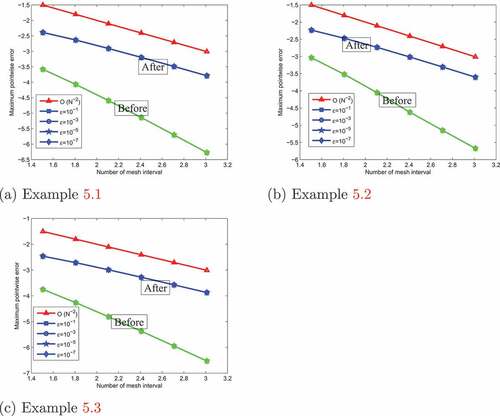As the size of $\delta$ increases, the thickness of the layer increases (see, Figures 2(a), 2 (2)), whereas when the size of $\eta$ increases, the thickness of the layer decreases (see, Figures 3(a) 3 (3)). Figures 4, Figure 5 and Figure 6 depict the 3D view of the numerical solution profiles for Examples 5.1, 5.2 and 5.3, respectively, which indicates the existence of the boundary layer near x = 1. In Figure 7(a),(7) 7 (7), we have plotted the maximum pointwise errors (before and after extrapolation) in a log-log plot for Examples 5.1–5.3, which show that the expected numerical order of convergence is correct in practice.

Table 1. $E_{\epsilon ,\delta ,\eta }^{N,\tau },r_{\epsilon ,\delta ,\eta }^{N,\tau }$ $E^{N,\tau }$, $r^{N,\tau }$ $(E_{\epsilon ,\delta ,\eta }^{N,\tau })extp$ $(r_{\epsilon ,\delta ,\eta }^{N,\tau })extp$, $(E^{N,\tau })extp$ and $(r^{N,\tau })extp$ for Example, 5.1 using method (3.19) and scheme(3.19) with Richardson extrapolation (4.10) with $\delta =\eta =0.5\times \epsilon$

$\epsilon \downarrow$	M = N =$2^5$	$2^6$	$2^7$	$2^8$	$2^9$	$2^{10}$
Before Richardson extrapolation
${10}^0$	1.6456e-04	8.3559e-05	4.2158e-05	2.1190e-05	1.0624e-05	5.3192e-06
	0.9777	0.9870	0.9924	0.9961	0.9980	0.9991
${10}^{-1}$	2.6401e-03	8.5806e-04	3.8791e-04	2.1162e-04	1.1057e-04	5.6525e-05
	0.8065	0.9082	0.9556	0.9783	0.9991	0.9994
${10}^{-3}$	4.0549e-03	2.3173e-03	1.2345e-03	6.3645e-04	3.2305e-04	1.6274e-04
	0.8072	0.9085	0.9558	0.9783	0.9892	0.9945
${10}^{-5}$	4.0537e-03	2.3165e-03	1.2341e-03	6.3621e-04	3.2292e-04	1.6267e-04
	0.8073	0.9085	0.9559	0.9783	0.9892	0.9945
${10}^{-7}$	4.0537e-03	2.3165e-03	1.2341e-03	6.3621e-04	3.2292e-04	1.6267e-04
	0.8073	0.9085	0.9559	0.9783	0.9892	0.9945
${10}^{-9}$	4.0537e-03	2.3165e-03	1.2341e-03	6.3621e-04	3.2292e-04	1.6267e-04
	0.8073	0.9085	0.9559	0.9783	0.9892	0.9945
$E^{N,\tau }$	4.0549e-03	2.3173e-03	1.2345e-03	6.3645e-04	3.2305e-04	1.6274e-04
$r^{N,\tau }$	0.8072	0.9085	0.9558	0.9783	0.9892	0.9945
After Richardson extrapolation
${10}^0$	2.5460e-05	6.3683e-06	1.5926e-06	3.9842e-07	1.0011e-07	2.6040e-08
	1.9993	1.9995	1.9990	1.9927	1.9428	1.9517
${10}^{-1}$	1.0766e-03	4.0666e-04	1.1307e-04	2.9173e-05	7.3984e-06	1.8591e-06
	1.4046	1.8466	1.9545	1.9793	1.9926	1.9973
${10}^{-3}$	2.6218e-04	8.5570e-05	2.5624e-05	7.2641e-06	1.9867e-06	5.3256e-07
	1.6154	1.7396	1.8186	1.8704	1.8994	1.8995
${10}^{-5}$	2.6202e-04	8.5513e-05	2.5606e-05	7.2587e-06	1.9852e-06	5.3216e-07
	1.6155	1.7397	1.8187	1.8693	1.8994	1.8994
${10}^{-7}$	2.6202e-04	8.5513e-05	2.5606e-05	7.2587e-06	1.9852e-06	5.3216e-07
	1.6155	1.7397	1.8187	1.8693	1.8994	1.8994
${10}^{-9}$	2.6202e-04	8.5513e-05	2.5606e-05	7.2587e-06	1.9852e-06	5.3216e-07
	1.6155	1.7397	1.8187	1.8693	1.8994	1.8994
$(E^{N,\tau })extp$	2.6218e-04	8.5570e-05	2.5624e-05	7.2641e-06	1.9867e-06	5.3256e-07
$(r^{N,\tau })extp$	1.6154	1.7396	1.8186	1.8704	1.8994	1.8995
Results in (Kumar, 2018)
$E^{N,\tau }$	4.71e-03	2.84e-03	1.68e-03	9.56e-04	5.41e-04	2.88e-04
$r^{N,\tau }$	0.73	0.76	0.81	0.85	0.88

Table 2. $E_{\epsilon ,\delta ,\eta }^{N,\tau },r_{\epsilon ,\delta ,\eta }^{N,\tau }$ $E^{N,\tau }$, $r^{N,\tau }$ $(E_{\epsilon ,\delta ,\eta }^{N,\tau })extp$ $(r_{\epsilon ,\delta ,\eta }^{N,\tau })extp$, $(E^{N,\tau })extp$ and $(r^{N,\tau })extp$ for Example, 5.2 using method (3.19) and scheme(3.19) with Richardson extrapolation (4.10) with $\delta =\eta =0.5\times \epsilon ,M=N$

$\epsilon \downarrow$	M = N =$2^5$	$2^6$	$2^7$	$2^8$	$2^9$	$2^{10}$
Before Richardson extrapolation
${10}^0$	1.6456e-04	8.3559e-05	4.2158e-05	2.1190e-05	1.0624e-05	5.3192e-06
	0.70344	0.83740	0.91361	0.95774	0.97784	0.98898
${10}^{-1}$	2.6401e-03	8.5806e-04	3.8791e-04	2.1162e-04	1.1057e-04	5.6525e-05
	0.92139	0.95697	0.97447	0.98656	0.99296	0.99639
${10}^{-3}$	4.0549e-03	2.3173e-03	1.2345e-03	6.3645e-04	3.2305e-04	1.6274e-04
	0.78380	0.87780	0.93429	0.96595	0.98276	0.99137
${10}^{-5}$	4.0537e-03	2.3165e-03	1.2341e-03	6.3621e-04	3.2292e-04	1.6267e-04
	0.78374	0.87781	0.93421	0.96596	0.98273	0.99131
${10}^{-7}$	4.0537e-03	2.3165e-03	1.2341e-03	6.3621e-04	3.2292e-04	1.6267e-04
	0.78374	0.87781	0.93421	0.96596	0.98273	0.99131
${10}^{-9}$	4.0537e-03	2.3165e-03	1.2341e-03	6.3621e-04	3.2292e-04	1.6267e-04
	0.78374	0.87781	0.93421	0.96596	0.98273	0.99131
$E^{N,\tau }$	4.0549e-03	2.3173e-03	1.2345e-03	6.3645e-04	3.2305e-04	1.6274e-04
$r^{N,\tau }$	0.78380	0.87780	0.93429	0.96595	0.98276	0.99137
After Richardson extrapolation
${10}^0$	2.5460e-05	6.3683e-06	1.5926e-06	3.9842e-07	1.0011e-07	2.6040e-08
	1.4282	1.4857	1.6461	1.6667	1.8179	1.9023
${10}^{-1}$	1.0766e-03	4.0666e-04	1.1307e-04	2.9173e-05	7.3984e-06	1.8591e-06
	1.5447	1.8354	1.9325	1.9696	1.9881	2.0165
${10}^{-3}$	2.6218e-04	8.5570e-05	2.5624e-05	7.2641e-06	1.9867e-06	5.3256e-07
	1.5998	1.7718	1.8846	1.7577	1.7410	1.8092
${10}^{-5}$	2.6202e-04	8.5513e-05	2.5606e-05	7.2587e-06	1.9852e-06	5.3216e-07
	1.5996	1.7717	1.8845	1.7573	1.7408	1.8091
${10}^{-7}$	2.6202e-04	8.5513e-05	2.5606e-05	7.2587e-06	1.9852e-06	5.3216e-07
	1.5996	1.7717	1.8845	1.7573	1.7408	1.8091
${10}^{-9}$	2.6202e-04	8.5513e-05	2.5606e-05	7.2587e-06	1.9852e-06	5.3216e-07
	1.5996	1.7717	1.8845	1.7573	1.7408	1.8091
$(E^{N,\tau })extp$	2.6218e-04	8.5570e-05	2.5624e-05	7.2641e-06	1.9867e-06	5.3256e-07
$(r^{N,\tau })extp$	1.5998	1.7718	1.8846	1.7577	1.7410	1.8092
Results in (Woldaregay & Duressa, 2022)
$E^{N,M}$	5.7389e-03	2.9180e-03	1.4718e-03	7.3915e-04	3.7036e-04	1.8537e-04
$r^{N,M}$	0.9758	0.9874	0.9936	0.9969	0.9985

Table 3. $E_{\epsilon ,\delta ,\eta }^{N,\tau },r_{\epsilon ,\delta ,\eta }^{N,\tau }$ $E^{N,\tau }$, $r^{N,\tau }$ $(E_{\epsilon ,\delta ,\eta }^{N,\tau })extp$ $(r_{\epsilon ,\delta ,\eta }^{N,\tau })extp$, $(E^{N,\tau })extp$ and $(r^{N,\tau })extp$ for Example, 5.3 using method (3.19) and method (3.19) with Richardson extrapolation (4.10) with $T=1.0,\delta =\eta =0.5\times \epsilon$

$\epsilon \downarrow$	M = N =$2^5$	$2^6$	$2^7$	$2^8$	$2^9$	$2^{10}$
Before Richardson extrapolation
${10}^0$	1.4289e-04	7.2851e-05	3.6796e-05	1.8501e-05	9.2775e-06	4.6456e-06
	0.97188	0.98540	0.99195	0.99580	0.99787	0.99894
${10}^{-1}$	2.3424e-03	7.6429e-04	2.6867e-04	1.4594e-04	7.6134e-05	3.8891e-05
	1.6158	1.5083	0.88046	0.93876	0.96910	0.99730
${10}^{-3}$	3.4414e-03	1.9307e-03	1.0206e-03	5.2439e-04	2.6575e-04	1.3377e-04
	0.83387	0.91971	0.96071	0.98057	0.99032	0.99511
${10}^{-5}$	3.4409e-03	1.9304e-03	1.0204e-03	5.2428e-04	2.6569e-04	1.3374e-04
	0.83389	0.91977	0.96073	0.98059	0.99031	0.99511
${10}^{-7}$	3.4409e-03	1.9304e-03	1.0204e-03	5.2428e-04	2.6569e-04	1.3374e-04
	0.83389	0.91977	0.96073	0.98059	0.99031	0.99511
${10}^{-9}$	3.4409e-03	1.9304e-03	1.0204e-03	5.2428e-04	2.6569e-04	1.3374e-04
	0.83389	0.91977	0.96073	0.98059	0.99031	0.99511
$E^{N,\tau }$	3.4414e-03	1.9307e-03	1.0206e-03	5.2439e-04	2.6575e-04	1.3377e-04
$r^{N,\tau }$	0.83387	0.91971	0.96071	0.98057	0.99032	0.99511
After Richardson extrapolation
${10}^0$	2.1652e-05	5.4163e-06	1.3544e-06	3.3884e-07	8.5148e-08	2.2156e-08
	1.9991	1.9997	1.9990	1.9926	1.9423	1.9958
${10}^{-1}$	9.2273e-04	3.5453e-04	9.9234e-05	2.5594e-05	6.4552e-06	1.6121e-06
	1.380	1.8370	1.9550	1.9873	2.0015	2.0000
${10}^{-3}$	1.7787e-04	5.4339e-05	1.5487e-05	4.2335e-06	1.1276e-06	2.9713e-07
	1.7108	1.8109	1.8711	1.9086	1.9241	1.9758
${10}^{-5}$	1.7777e-04	5.4303e-05	1.5477e-05	4.2308e-06	1.1269e-06	2.9708e-07
	1.7109	1.8109	1.8711	1.9086	1.9234	1.9761
${10}^{-7}$	1.7777e-04	5.4303e-05	1.5477e-05	4.2308e-06	1.1269e-06	2.9708e-07
	1.7109	1.8109	1.8711	1.9086	1.9234	1.9761
${10}^{-9}$	1.7777e-04	5.4303e-05	1.5477e-05	4.2308e-06	1.1269e-06	2.9708e-07
	1.7109	1.8109	1.8711	1.9086	1.9234	1.9761
$(E^{N,\tau })extp$	1.7787e-04	5.4339e-05	1.5487e-05	4.2335e-06	1.1276e-06	2.9713e-07
$(r^{N,\tau })extp$	1.7108	1.8109	1.8711	1.9086	1.9241	1.9758

Table 4. $(E_{\epsilon ,\delta ,\eta }^{N,\tau })extp$ $(r_{\epsilon ,\delta ,\eta }^{N,\tau })extp$, $(E^{N,\tau })extp$ and $(r^{N,\tau })extp$ for Example, 5.1 using proposed method (3.19) with Richardson extrapolation (4.10) and results in (Mesfin M. Woldaregay & Duressa, 2019) and (Woldaregay & Duressa, 2020) with $T=3,\delta =0.6\times \epsilon ,\eta =0.5\times \epsilon$

$\epsilon \downarrow$ $N\to$	$2^5$	$2^6$	$2^7$	$2^8$	$2^9$
$M\to$	60	120	240	480	960
Proposed scheme in (4.10)
$2^{-6}$	3.6301e-04	1.2211e-04	3.8062e-05	2.2568e-05	3.7270e-05
	1.5718	1.6818	1.5986	1.7537
$2^{-8}$	3.5832e-04	1.2075e-04	3.7798e-05	1.2027e-05	3.6040e-06
	1.5692	1.6756	1.6520	1.7386
$2^{-10}$	3.5756e-04	1.2041e-04	3.7740e-05	1.2012e-05	3.5980e-06
	1.5702	1.6738	1.6516	1.7392
$2^{-12}$	3.5737e-04	1.2032e-04	3.7725e-05	1.2008e-05	3.5964e-06
	1.5705	1.6733	1.6515	1.7394
$2^{-14}$	3.5732e-04	1.2030e-04	3.7721e-05	1.2007e-05	3.5960e-06
	1.5706	1.6732	1.6515	1.7394
$2^{-16}$	3.5731e-04	1.2029e-04	3.7720e-05	1.2006e-05	3.5959e-06
	1.5707	1.6731	1.6516	1.7393
$2^{-18}$	3.5730e-04	1.2029e-04	3.7720e-05	1.2006e-05	3.5959e-06
	1.5707	1.6731	1.6516	1.7393
$2^{-20}$	3.5730e-04	1.2029e-04	3.7720e-05	1.2006e-05	3.5959e-06
	1.5707	1.6731	1.6516	1.7393
$(E^{N,\tau })extp$	3.6301e-04	1.2211e-04	3.8062e-05	2.2568e-05	3.7270e-05
$(r^{N,\tau })extp$	1.5718	1.6818	1.5986	1.7537
Results in (Mesfin M. Woldaregay & Duressa, 2019)
$E^{N,M}$	9.7515e-03	4.8801e-03	2.4414e-03	1.2211e-03	6.1064e-04
$r^{N,M}$	9.9874e-01	9.9917e-01	9.9958e-01	9.9976e-01
Results in (Woldaregay & Duressa, 2020)
$E^{N,M}$	4.7005e-03	2.3806e-03	1.1976e-03	6.0058e-04	3.0073e-04
$r^{N,M}$	9.9871e-01	9.9920e-01	9.9953e-01	9.9979e-01

Figure 1. The effect of $\epsilon$ on the solution profiles at $\delta =0.6\times \epsilon$ and $\eta =0.5\times \epsilon$.

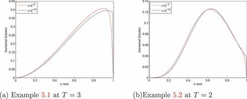
Figure 2. The effect of $\delta$ on the solution profiles at $\epsilon =2^{-4},\eta =0.5\times \epsilon$.

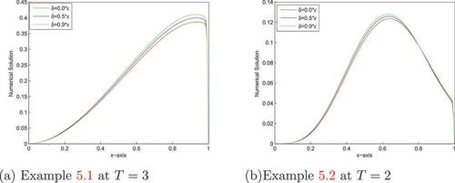
Figure 3. The effect of $\eta$ on the solution profiles with $\epsilon =2^{-4},\delta =0.6\times \epsilon$.

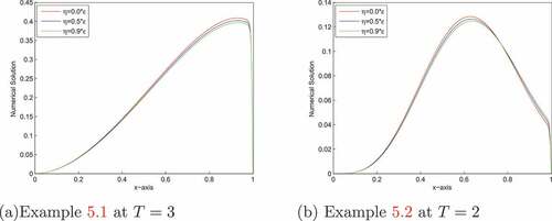
Figure 4. Numerical solution profiles for Example, 5.1 at $\delta =0.6\times \epsilon ,\eta =0.5\times \epsilon ,N=M=512$.

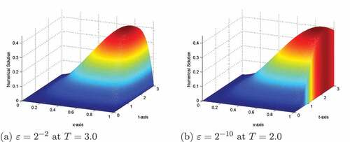
Figure 5. Numerical solution profiles for Example, (5.2) at $T=2.0,\delta =0.6\times \epsilon ,\eta =0.5\times \epsilon$ and $N=M=512$.

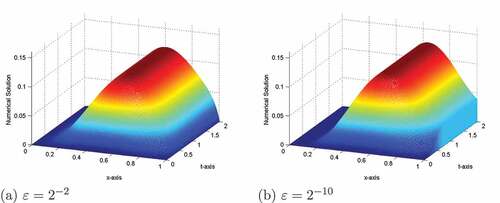
Figure 6. Numerical solution profiles for Example, 5.3 at $T=1.0,\delta =0.6\times \epsilon ,\eta =0.5\times \epsilon$ and $N=M=512$.

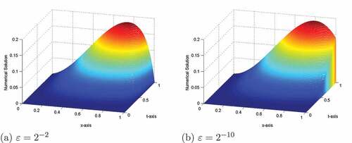
Figure 7. Log-log plot for the maximum absolute errors before and after the Richardson extrapolation technique.

6 Conclusion

In this paper, a higher-order robust numerical scheme has been proposed to solve singularly perturbed parabolic differential-difference equations with mixed shifts in the space variable. The scheme comprises of the implicit Euler method to discretize the temporal variable and the cubic spline in tension method to discretize the spatial variable on a uniform step length. Besides this, Richardson’s extrapolation technique has been implemented to enhance the accuracy in the temporal direction. Stability and uniform convergence of the proposed scheme have been investigated. The scheme has been shown uniformly convergent with linear order of convergence before Richardson extrapolation and second order convergent after Richardson extrapolation. Several model examples have been presented to illustrate the efficiency of the proposed method. It has been observed that the proposed scheme gives high accurate numerical results and higher order of convergence than the methods in (Kumar, 2018; Mesfin M. Woldaregay & Duressa, 2019; Woldaregay & Duressa, 2020, 2022). The proposed method is can be successfully applied for similar singularly perturbed parabolic partial differential problems with shift parameter(s) and without delay parameter. But, the proposed scheme is not a layer resolving method. In future works, we extend the proposed scheme for singularly perturbed problems with degenerate coefficients and singularly perturbed problems with nonlocal boundary conditions.

Acknowledgements

The authors thankfully acknowledge the prolific comments from the anonymous referees.

Disclosure statement

No potential conflict of interest was reported by the author(s).

Data availability statement

No data were used to support the study.

Additional information

Funding

This research did not receive any funding.

Notes on contributors

Imiru Takele Daba

Imiru Takele Daba received his Ph.D. in Mathematics from Wollega University in 2021. Currently, he is working at Dilla University, Department of Mathematics as a researcher and assistant professor. His research interests span the areas of numerical solution of partial differential equations, focusing on singularly perturbed problems. He has published more than seven research articles in reputable journals. He also made numerous contributions in serving as a reviewer. So far, he has supervised five M.Sc. students to completion and currently supervising six M.Sc. students.

Gemechis File Duressa

Gemechis File Duressa received his Ph.D. in Mathematics from the National Institute of Technology Warangal, India, in 2014. He is presently working at Jimma University as a full professor of Mathematics and Dean, College of Natural Sciences, Jimma University, Ethiopia. His research interests span on the areas of numerical solution of differential equations, mainly, on singularly perturbed ordinary and partial differential equations. He published more than 130 research articles in national and international reputable journals. In addition, he made numerous contributions in serving as reviewer, assistant editor, and editor for various national and international reputable journals. So far, he has supervised 40 M.Sc. and 7 Ph.D. graduates to completion and currently supervising five M.Sc. students and 15 Ph.D. scholars.

References

- Andre Longtin, J. G. M. (1988). Complex oscillations in the human pupil light reflex with mixed and delayed feedback. Mathematical Biosciences, 90(1–2), 183–16. https://doi.org/10.1016/0025-5564(88)90064-8
- Bansal, K., & Kapil, K. (2017). Sharma Parameter uniform numerical scheme for time dependent singularly perturbed convection-diffusion-reaction problems with general shift arguments. Numerical Algorithms, 75(1), 113–145. https://doi.org/10.1007/s11075-016-0199-3
- Bansal, K., & Pratima Rai, K. K. S. (2017). Numerical treatment for the class of time dependent singularly perturbed parabolic problems with general shift arguments. Differential Equations and Dynamical Systems, 25(2), 327–436. https://doi.org/10.1007/s12591-015-0265-7
- Culshaw, R. V., & Ruan, S. (2000). A delay-differential equation model of HIV infection of CD4+ T-cells. Mathematical Biosciences, 165(1), 27–39. https://doi.org/10.1016/S0025-5564(00)00006-7
- Daba, I. (2021a). Takele and Duressa, gemechis file, extended cubic B-spline collocation method for singularly perturbed parabolic differential-difference equation arising in computational neuroscience. International Journal for Numerical Methods in Biomedical Engineering, 37(2), e3418. https://doi.org/10.1002/cnm.3418
- Daba, I. (2021b). Takele and Duressa, gemechis file,hybrid algorithm for singularly perturbed delay parabolic partial differential equations. Applications and Applied Mathematics: An International Journal (AAM), 16(1), 21. http://pvamu.edu/aam.
- Daba, I. (2021c). Takele and Duressa, Gemechis file, A hybrid numerical scheme for singularly perturbed parabolic differential-difference equations arising in the modeling of neuronal variability. Computational and Mathematical Methods, 3(5), e1178. https://doi.org/10.1002/cmm4.1178
- Daba, I. (2021d). Takele and Duressa, Gemechis file, uniformly convergent numerical scheme for a singularly perturbed differential-difference equations arising in computational neuroscience. Journal of Applied Mathematics and Informatics, 39(5–6), 655–676. https://doi.org/10.1002/cmm4.1178
- Daba, I. (2022a). Takele and Duressa, Gemechis file. Collocation Method Using Artificial Viscosity for Time Dependent Singularly Perturbed differential–difference Equations Mathematics and Computers in Simulation, 192, 201–220,. https://doi.org/10.1002/cmm4.1178
- Daba, I. (2022b). Takele and Duressa, Gemechis File,A Robust computational method for singularly perturbed delay parabolic convection-diffusion equations arising in the modeling of neuronal variability. Computational Methods for Differential Equations, 10(2), 475–488. https://cmde.tabrizu.ac.ir/article_12797.html
- Derstine, M. W., Gibbs, H. M., Hopf, F. A., & Kaplan, D. L. (1982). Bifurcation gap in a hybrid optically bistable system. Physical Review A, 26(6), 3720–3722. https://doi.org/10.1103/PhysRevA.26.3720
- Edward, P. D., John, J. H., & Miller, Willy, H. A. (1980). Schilders, Uniform numerical methods for problems with initial and boundary layers. Boole Press.
- Glizer, V. Y. (2000). Asymptotic solution of a boundary-value problem for linear singularly-perturbed functional differential equations arising in optimal control theory. Journal of Optimization Theory and Applications, 106(2), 309–335. https://doi.org/10.1023/A:1004651430364
- Glizer, V. Y. (2003). Blockwise estimate of the fundamental matrix of linear singularly perturbed differential systems with small delay and its application to uniform asymptotic solution. Journal of Mathematical Analysis and Applications, 278(2), 409–433. https://doi.org/10.1016/S0022-247X(02)00715-1
- John Mallet-Paret, R. D. (1989). Nussbaum. A differential-delay Equation Arising in Optics and Physiology, SIAM Journal on Mathematical Analysis, 20(2), 249–292. https://doi.org/10.1137/0520019
- John Wilbur, W., & Rinzel, J. (1982). An analysis of Stein’s model for stochastic neuronal excitation. Biological Cybernetics, 45(2), 107–114. https://doi.org/10.1007/BF00335237
- Khan, A., Khan, I., & Tariq Aziz, M. (2004). Stojanovic. A variable-mesh Approximation Method for Singularly Perturbed boundary-value Problems Using Cubic Spline in Tension, International Journal of Computer Mathematics, 81(12), 1513–1518. https://doi.org/10.1080/00207160412331284169
- Kostikov, Y. A., & Romanenkov, A. M. (2020). Approximation of the multidimensional optimal control problem for the heat equation (applicable to computational fluid dynamics (CFD)). Civil Engineering Journal, 6(4), 743–768. https://doi.org/10.28991/cej-2020-03091506
- Kot, M. (2001). Elements of mathematical ecology. Cambridge University Press.
- Kuang, Y. (1993). Delay differential equations: With applications in population dynamics. cademic press.
- Kumar, D. (2018). An implicit scheme for singularly perturbed parabolic problem with retarded terms arising in computational neuroscience. Numerical Methods for Partial Differential Equations, 34(6), 1933–1952. https://doi.org/10.1002/num.22269
- Kumar, M., & Gupta, Y. (2010). Methods for solving singular boundary value problems using splines: A review. Journal of Applied Mathematics and Computing, 32(1), 265–278. https://doi.org/10.1007/s12190-009-0249-2
- Ladyzhenskaia, O. A., Solonnikov, V. A., & Nina, N. (1968). Ural’tseva, Linear and quasi-linear equations of parabolic type, 23. American Mathematical Soc.
- Lánskỳ, P. (1984). On approximations of Stein’s neuronal model. Journal of Theoretical Biology, 107(4), 631–647. https://doi.org/10.1016/S0022-5193(84)80136-8
- Mackey, M. C., & Glass, L. (1977). Oscillation and chaos in physiological control systems. Science, 197(4300), 287–289. https://doi.org/10.1126/science.267326
- Mayer, H., Zaenker, K. S., & An Der Heiden, U. (1995). A basic mathematical model of the immune response, Chaos: An interdisciplinary. Journal of Nonlinear Science, 5(1), 155–161. https://aip.scitation.org/doi/abs/10.1063/1.166098
- MihajloviC, G., & Zivkovic, M. (2020). Sieving extremely wet earth mass by means of oscillatory transporting platform. Emerging Science Journal, 4(3), 172–182. https://doi.org/10.28991/esj-2020-01221
- Murray, J. D. (2007). Mathematical biology: I. An Introduction, 17. https://link.springer.com/content/pdf/10.1007/b98868.pdf%20http://www.ulb.tu-darmstadt.de/tocs/127987207.pdf
- Musila, M., & Lánskỳ, P. (1991). Generalized Stein’s model for anatomically complex neurons. BioSystems, 25(3), 179–191. https://doi.org/10.1016/0303-2647(91)90004-5
- Nageshwar Rao, R., & Pramod Chakravarthy, P. (2019). Fitted numerical methods for singularly perturbed one-dimensional parabolic partial differential equations with small shifts arising in the modelling of neuronal variability. Differential Equations and Dynamical Systems, 27(1–3), 1–18. https://doi.org/10.1007/s12591-017-0363-9
- Nelson, P. W., & Perelson, A. S. (2002). Mathematical analysis of delay differential equation models of HIV-1 infection. Mathematical Biosciences, 179(1), 73–94. https://doi.org/10.1016/S0025-5564(02)00099-8
- Nichols, N. K. (1989). On the numerical integration of a class of singular perturbation problems. Journal of Optimization Theory and Applications, 60(3), 439–452. https://doi.org/10.1007/BF00940347
- O’Malley, R. E. (1991). Singular perturbation methods for ordinary differential equations. New York: Springer.
- Pramod Chakravarthy, P., Dinesh Kumar, S., & Nageshwar Rao, R. (2017). Numerical solution of second order singularly perturbed delay differential equations via cubic spline in tension. International Journal of Applied and Computational Mathematics, 3(3), 1703–1717. https://doi.org/10.1007/s40819-016-0204-5
- Ramesh, V. P., & Priyanga, B. (2019). Higher order uniformly convergent numerical algorithm for time-dependent singularly perturbed differential-difference equations, (pp. 1–25). Differential Equations and Dynamical Systems.
- Ravi Kanth, A. S. V., Murali, P., & Mohan, K. (2017). A numerical approach for solving singularly perturbed convection delay problems via exponentially fitted spline method. Calcolo, 54(3), 943–961. https://doi.org/10.1007/s10092-017-0215–6
- Stein, R. B. (1967). Some models of neuronal variability. Biophysical Journal,7(1), 7(1), 37–68. https://doi.org/10.1016/S0006-3495(67)86574-3
- Tene, T., Guevara, M., Svozil, J., Tene-Fernandez, R., & Gomez, C. V. (2021). Analysis of covid-19 outbreak in Ecuador using the logistic model. Emerging Science Journal, 5, 105–118. https://doi.org/10.28991/esj-2021-SPER-09
- Vikas Gupta, M. K., & Kadalbajoo, R. K. (2019). Dubey. A parameter-uniform Higher Order Finite Difference Scheme for Singularly Perturbed time-dependent Parabolic Problem with Two Small Parameters, International Journal of Computer Mathematics, 96(3), 474–499. https://doi.org/10.1080/00207160.2018.1432856
- Wazewska-Czyzewska, M., & Lasota, A. (9176). Mathematical models of the red cell system. Matematyta Stosowana, 6(1), 25–40.
- Woldaregay, M. M., & Duressa, G. F. (2019). Parameter uniform numerical method for singularly perturbed parabolic differential difference equations. Journal of the Nigerian Mathematical Society, 38(2), 223–245. https://ojs.ictp.it/jnms/index.php/jnms/article/view/474
- Woldaregay, M. M., & Duressa, G. F. (2020). Uniformly convergent numerical scheme for singularly perturbed parabolic delay differential equations. ITM Web of Conferences, 34, 02011. https://doi.org/10.1051/itmconf/20203402011
- Woldaregay, M. M., & Duressa, G. F. (2022). Uniformly convergent numerical method for singularly perturbed delay parabolic differential equations arising in computational neuroscience. Kragujevac Journal of mathematics, 46(1), 65–84.