Analysis of thermal and surface roughness effects of slider bearing in the case of turbulent lubricant flow using finite element method

ABSTRACT

In this study, the effects of surface roughness and thermal on slider bearings with turbulent fluid film were examined using the Streamline Upwind Petrov–Galerkin (SUPG)-Finite Element Method. Using the assumption that roughness is stochastic and has a Gaussian random distribution, one-dimensional transverse and longitudinal surface roughness models were taken into consideration. The texture of the surface’s irregularity is changed into a regular domain for computational efficiency. To derive the modified Reynolds equation for turbulent lubrication, the Ng-Pan turbulent model is used. For all local Reynolds values, the pressure distribution of the combined effect is less than the thermal and surface roughness influences of the one-dimensional longitudinal surface roughness, which is a reduction of 16% in load-carrying capacity performance and 3% decrease in friction force, for non-parallel (w = 0.4) between the surface roughness effect and the combined effect condition, respectively. However, the pressure distribution of the thermal effect is smaller than the combined and surface roughness effects in the transverse, one-dimensional roughness model for all local Reynolds values, which is a reduction of 33% in load–carrying capacity performance and 13% decrease in friction force, for non-parallel (w = 0.4) between the surface roughness effect and the thermal effect condition, respectively. Moreover, the combined effects at various temperatures are examined. As a result, the load-carrying capacity performance is better in the case where the pad temperature is lower than the slider in both longitudinal and transverse models. The performance of a slider bearing will generally be improved by taking surface roughness and the coefficients of turbulent lubrication equations into account. Tables and figures were used to present the results.

KEYWORDS:

• turbulent flow
• slider bearing
• longitudinal
• transverse
• load-carrying capacity
• pressure distribution
• finite element method

1. Introduction

Under turbulent flow conditions, slider bearings are among the most vital parts of a machine’s operating condition. Bearings must be capable of supporting increased levels of stress and strain when operating in turbulent flow conditions. Higher levels of stress and strain necessitate higher-performance bearings, which must be more durable and reliable in order to perform effectively. From engineering to the automotive industry, the geometry of a rough slider bearing is critical. Furthermore, the geometry influences the load capacity and wear characteristics of the bearing. As a result, understanding the bearing’s geometry is critical for any successful application.

The use of slider bearings in turbulent flows poses special challenges because turbulence can cause the formation of eddies or vortices that disrupt the hydrodynamic lubrication film. One of the most critical aspects of designing a slider bearing for turbulent fluid flow is ensuring that the bearing is stiff enough to avoid dynamic instability. To be more specific, slider bearings are used in sliding motions between two surfaces, which helps to reduce friction and makes it possible for the suspension components to move more reliably and smoothly, resulting in effective operation and a longer equipment lifespan.

Several researchers have made attempts to build the turbulent lubrication hypothesis over the past more than half of a century. A theoretical solution to this issue was first developed by Constantinescu (1959) and was based on Prandtl’s mixing length notion. A linearized theory of turbulent lubrication was developed by Ng and Pan (1965) using the Reichardt formula for eddy viscosity. In the latter, Elrod and Ng (1967) expanded on the work of Ng and Pan to enable the application of both pressure and shear fluxes to the combined lubricant flow. Burton (1974) and Black (1970) used the knowledge of the contour of the time-averaged flow velocity profile in the lubricant film to arrive at a simpler method. By utilizing the correlations between wall shear stress and mean velocity relative to the wall, Hirs (1973) established a brand-new technique based on the bulk flow notion. Moreover, Ho and Vohr (1974) used Kolmogorov’s turbulence energy model to calculate the velocity distribution in the turbulent film.

A new theoretical approach to turbulent lubrication problems, including the surface roughness effects, was described on fluid film bearing by Hashimoto and Wada (1989). Also, turbulence models of hydrodynamic lubrication by Zhang et al. (2003), on a journal bearing the course of their development and their fundamentals, were explained. Some researchers have studied various types of bearings with surface roughness effects, like Lin (2000) studied hydrostatic bearings, Guha (2000) studied journal bearings, and Christensen and Tonder (1971) the slider bearings. Kumar (2001) analyzed a segregated FEM of the Petrov–Galerkin framework with suitably SUPG weight functions for a non-isothermal flow with temperature-dependent density and viscosity in a high-speed slider bearings model. Rathish Kumar and Srinivasa Rao (2000) investigated the numerical simulation of slider bearings of load-carrying support using the SUPG-FEM.

For a finite width plane inclined slider thrust-bearing hydrodynamically lubricated with an isoviscous incompressible fluid, Taylor (1969) compares the quantitative predictions of two main engineering approaches and evaluates a method available to the fluid film-bearing designer to examine turbulent flow conditions and the effect of turbulence. King and Taylor (1977) studied the effect of fluid inertia on the performance of the plane-inclined slider bearing with turbulent lubrication. Belhocine and Abdullah (2019) studied the numerical simulation of thermally developing turbulent flow through a cylindrical tube. Belhocine et al. (2022), Belhocine and Omar (2021), and Belhocine et al. (2021) are some of the papers studied on laminar flow. In addition, Belhocine and Afzal (2022) and Belhocine and Omar (2017) used finite element analysis on brake disc by using the finite element software ANSYS 11.0 to obtain numerical results.

Lahmar et al. (2013) were investigating the homogenization method of roughness analysis in turbulent lubrication. In their works, journal bearings with a rough surface operating in the turbulent regime were analyzed. A numerical investigation of turbulence models for a superlaminar journal bearing by Ding et al. (2018) with rotating machines working at high speeds was analyzed through computational fluid dynamics. Wang et al. (2020) studied the performance of high-speed hydrodynamic journal bearings with lubricating oils combining laminar and turbulent flows. In their study, governing equations were solved by the finite difference method. Two-dimensional distributions of Reynolds number, pressure, and temperature in the bearing film, as well as lubrication characteristics like bearing capacity and frictional force under working conditions, were analyzed.

The finite difference method was used by Sinha and Adamu (2009) to analyze the thermo hydrodynamic analysis of an infinitely long tilted pad slider bearing with roughness. Adamu and Sinha (2012) with heat conduction through both the pad and slider, considering two models of one-dimensional longitudinal and transverse roughness, where surface roughness is assumed to be stochastic and Gaussian randomly distributed.

Recently, Desu Tessema et al. (2022) investigated the performance of slider bearings with the effects of temperature and surface roughness on one-dimensional longitudinal and transverse roughness types using the Streamline Upwind Petrov–Galerkin (SUPG)- finite element method (FEM). Singh et al. (2018) reported a numerical study of the hydrodynamic lubrication of slider bearings with textured surfaces. Overall, our literature review as well as our knowledge concerns indicates that we have not seen SUPG-FEM to solve the performance of slider bearings over combined thermal and surface roughness effects with turbulent fluid flow.

However, our significant contribution to this work is the formulation of the governing Reynolds equation for surface roughness (for one-dimensional longitudinal and transverse) with thermal impact for slider bearing, which is given in equations (12)(12) $\frac{\partial }{\partial x}\left[\frac{{\tilde{\overline{\rho }}}_{av}E\left(H^3\right)E\left(1/K_x\right)}{{\overline{\mu }}_{av}}\frac{\partial \tilde{\overline{p}}}{\partial x}\right]=\frac{U}{2}\frac{\partial ({\tilde{\overline{\rho }}}_{av}E(H))}{\partial x},$(12) and (18(18) $\frac{\partial }{\partial x}\left[\frac{{\tilde{\overline{\rho }}}_{av}}{{\tilde{\overline{\mu }}}_{av}E\left(1/H^3\right)E\left(K_x\right)}\frac{\partial \tilde{\overline{p}}}{\partial x}\right]=\frac{U}{2}\frac{\partial }{\partial x}\left(\frac{{\tilde{\overline{\rho }}}_{av}E\left(1/H^2\right)}{E\left(1/H^3\right)}\right).$(18) ). Little attention has been given to the combined impact of temperature and surface roughness on tilted pad slider bearings with turbulent fluid flow by SUPG-FEM. Thus, by taking into account the local Reynolds number effect, the combined effect of temperature and surface roughness on a slider bearing with the turbulent fluid film will be numerically analysed in this work using SUPG-FEM.

2. Governing equations

The geometry of a rough, long slider bearing is shown in Figure 1. When the length of the bearing is compared to the height of the fluid film thickness, it is infinitely long.

Figure 1. Geometry of one-dimensional slider bearing.

Source: https://www.hindawi.com/journals/mpe/2022/4216136/fig1

Each parameter in the Navier-Stokes equations for turbulent flow conditions is represented by a time mean value with a fluctuation around this mean value. As a result, a laminar flow is one in which the fluctuations are negligible in comparison to the mean overall flow. Thus, velocity (U, V), pressure (p), viscosity, density, and temperature are represented as the sum of a mean and fluctuating component.

(1) $\begin{array}{ll}& \mathrm{U}=\bar{\mathrm{u}}+{\mathrm{u}}^{\prime },\mathrm{V}=\bar{\mathrm{v}}+{\mathrm{v}}^{\prime },\mathrm{p}=\bar{\mathrm{p}}+{\mathrm{p}}^{\prime },\\ & \mathrm{T}=\bar{\mathrm{T}}+{\mathrm{T}}^{\prime },\mu =\overline{\mu }+{\mu }^{\prime },\rho =\overline{\rho }+{\rho }^{\prime },\end{array}$(1)

where the over-bar represents the average of the dependent variable and the prime denotes the fluctuation of the dependent variable due to turbulence. The chosen averaging method takes the mean values at a fixed point in space and averages them over a long enough time span that the mean values are independent of it. For example, for u velocity, the averaging is given below and in a similar way for the rest of the variables.

$\bar{\mathrm{u}}=\frac{1}{\mathrm{\Delta }\mathrm{t}}{\int }_0^{{\mathrm{t}}_0+{\mathrm{t}}_1}\mathrm{udt},$

where $\bar{\mathrm{u}}$ is time average of u. The time-averaged values of the fluctuating values are defined to be zero:

(2) $\begin{array}{ll}\overline{{\mathrm{u}}^{\prime }}=0,& \overline{{\mathrm{v}}^{\prime }}=0,\overline{{\mathrm{w}}^{\prime }}=0,\overline{{\mathrm{p}}^{\prime }}=0,\\ & \overline{{\mu }^{\prime }}=0,\overline{{\rho }^{\prime }}=0,\overline{{\mathrm{T}}^{\prime }}=0.\end{array}$(2)

In the turbulent regime, however, both Constantinescu and Ng and Pan disregard the terms corresponding to mean fluid inertia and base their assumptions on the fact that the lubricant is Newtonian, the fluid film thickness is significantly less than other bearing dimensions, body force is negligible, and there is no slip at the bearing surfaces. The general Navier-Stokes equations reduce to as given in Hooke (1999):

2.1. Equations of momentum

(3) $\frac{\partial }{\partial y}\left(\overline{\mu }\frac{\partial \overline{u}}{\partial y}\right)+\frac{\partial }{\partial y}(-\overline{\rho }\overline{u^{\prime }{v}^{\prime }})=\frac{d\overline{p}}{dx}.$(3)

With the exception of the second term, these equations are identical to those for the laminar regime. These additional stresses, in addition to the viscous stresses, are referred to as turbulent, apparent, or Reynolds stresses.

2.2. Equation of continuity

(4) $\frac{\partial }{\partial x}\left(\overline{\rho }\overline{u}\right)+\frac{\partial }{\partial y}\left(\overline{\rho }\overline{v}\right)=0.$(4)

To obtain the general Reynolds equation for turbulent flow, we combine equations (3)(3) $\frac{\partial }{\partial y}\left(\overline{\mu }\frac{\partial \overline{u}}{\partial y}\right)+\frac{\partial }{\partial y}(-\overline{\rho }\overline{u^{\prime }{v}^{\prime }})=\frac{d\overline{p}}{dx}.$(3) and (4(4) $\frac{\partial }{\partial x}\left(\overline{\rho }\overline{u}\right)+\frac{\partial }{\partial y}\left(\overline{\rho }\overline{v}\right)=0.$(4) ) using the boundary condition $u=U,v=0$ on the slider, $u=v=0$ on the pad, and replacing ρ by ρ_av and µ by µ_av.

Thus, the generalized Reynolds equation for turbulent flow is as follows:

2.3. Reynolds equation

(5) $\frac{\partial }{\partial x}\left(\frac{{\rho }_{av}{h}_t^3}{{\mu }_{av}{k}_x}\frac{dp}{dx}\right)={\displaystyle \frac{U}{2}}\frac{\partial }{\partial x}({\rho }_{av}{h}_t)+{\rho }_{av}\frac{\partial h_t}{\partial t},$(5)

where p is the turbulent flow film pressure, h_t is the nominal film thickness between smooth surfaces, U is the velocity of the moving surfaces, in the direction of the moving surface (x), t is time, and k_x are the turbulent lubrication equation coefficients. Although Ng and Pan (1965) provide the k_x curves as a function of the local Reynolds number Re, they cannot be used directly. Taylor and Dowson (1974) then replaced their curves with empirical k_x calculations, as shown in Equation (6(6) $k_x=12+A_{1}R{e}^{b_1},$(6) ).

(6) $k_x=12+A_{1}R{e}^{b_1},$(6)

where A₁ and b₁ are the turbulent lubrication model parameters, as shown in Table 1, and $Re=\rho U{h}_t/\mu$ is the local Reynolds number.

Table 1. NG-Pan parameters of turbulent model lubrication given in Taylor and Dowson (1974)

	A1	b1
50,000 ≤ Re	0.0388	0.8
10,000 ≤ Re ≤ 50,000	0.0250	0.84
5,000 ≤ Re ≤ 10,000	0.0250	0.84
1,000 ≤ Re ≤ 5,000	0.0039	1.06
Re ≤ 1,000	0.0000	0

For turbulent lubrication of a rough-surfaced bearing, the turbulent lubrication Equation (5)(5) $\frac{\partial }{\partial x}\left(\frac{{\rho }_{av}{h}_t^3}{{\mu }_{av}{k}_x}\frac{dp}{dx}\right)={\displaystyle \frac{U}{2}}\frac{\partial }{\partial x}({\rho }_{av}{h}_t)+{\rho }_{av}\frac{\partial h_t}{\partial t},$(5) must be satisfied at any local location on the bearing’s rough surface. As a result, the turbulent lubrication equation at any local position of the bearing with a rough surface can be obtained by applying the local film thickness under the actual surface profile to the Ng-Pan turbulent model.

(7) $\frac{\partial }{\partial x}\left(\frac{{\rho }_{av}{H}_t^3}{{\mu }_{av}{K}_x}\frac{dp}{dx}\right)={\displaystyle \frac{U}{2}}\frac{\partial }{\partial x}({\rho }_{av}{H}_t)+{\rho }_{av}\frac{\partial H_t}{\partial t},$(7)

In this formula, K_x is the turbulent lubrication equation coefficient, and H_t is the lubrication local film thickness. K_x can be obtained by replacing h_t with H_t in the k_x expressions.

(8) $K_x=12+A_{1}R{e}^{b_1}{\left[\frac{H_t}{h_t}\right]}^{b_1}.$(8)

The local film thickness H_t can be expressed as

(9) $H_t(x,z,t)=h_t(x,z,t)+{\delta }_s(x,z,ϵ),$(9)

where $h_t(x,z,ϵ)$ denotes the random component of the local film thickness to the surface asperity measured from the nominal mean level. The random variable ϵ describes a definite roughness arrangement (because a specific value of ϵ indicates that a roughness arrangement is randomly extracted from a large number of similar roughness arrangements with equal probability of having the same statistical parameters, the random variable ϵ obeys a uniform distribution). Since the contour height of the machined surface is close to the Gauss distribution, the roughness (the profile height distribution) studied in this paper is regarded as the Gauss distribution. As a result, the random variable δ_s has a Gaussian distribution.

In addition to the lubrication assumption mentioned above, the following assumptions are taken into account to obtain the energy equation as given in (Kumar, 2001; Rathish Kumar & Srinivasa Rao, 2000), and (Sinha & Adamu, 2009).

1. Other than those across the fluid film, conduction terms are negligible.

2. Thermal conductivity and specific heat are constants.

2.4. Energy equation

(10) $\overline{\rho }(\overline{u}\frac{\partial \overline{T}}{\partial x}+\overline{v}\frac{\partial \overline{T}}{\partial y})=k\frac{{\partial }^2\overline{T}}{\partial y^2}+\mu {\left(\frac{\partial \overline{u}}{\partial y}\right)}^2+\overline{u}\frac{\partial \overline{P}}{\partial x},$(10)

The lubricant’s viscosity and density are assumed to be temperature dependent and are expressed using the following equations:

$\rho ={\rho }_0(1-\lambda (\overline{T}-{\overline{T}}_a)),{\rho }_{av}={\rho }_a(1-\lambda ({\overline{T}}_{av}-{\overline{T}}_a)),$

where λ denotes the coefficient of thermal expansion, a denotes an ambient condition, and ρ and ρ_a denote the density at temperature $\overline{T}$ and ambient temperature ${\overline{T}}_a$, respectively.

$\begin{array}{ll}\mu =& {\mu }_{0}exp[-\beta (\overline{T}-{\overline{T}}_a)],\\ {\mu }_{av}=& {\mu }_{a}exp[-\beta ({\overline{T}}_{av}-{\overline{T}}_a)].\end{array}$

where µ and µ_a are the viscosity at $\overline{T}$ and ${\overline{T}}_a$ temperatures, respectively, and β is the temperature-viscosity coefficient, both at ambient pressure.

2.5. Basic assumptions

The details of the basic assumptions we have used are given in (Christensen, 1969), (Sinha & Adamu, 2009), and (Zhu et al., 2019). This paper employs two basic assumptions proposed by Christensen (1969) to deal with one-dimensional rough surface topography. The turbulent lubrication model with a one-dimensional longitudinal rough surface and a one-dimensional transverse rough surface is built on three fundamental assumptions:

Let n represent the direction perpendicular to the surface roughness direction and m represent the direction parallel to the surface roughness direction.

a.	The deterministic variable, the pressure gradient in the roughness direction ($\frac{\partial p}{\partial m}$) will be assumed (or the variance of the stochastic variable $\frac{\partial P}{\partial n}$ will be zero).
b.	The variable qm (the unit flow perpendicular to the surface roughness direction) will be assumed to be deterministic (or the variance of the stochastic variable qn is zero).
c.	The following velocity and temperature assumptions were improved by Sinha and Adamu (2009). The magnitudes of temperature and velocity associated with roughness are insignificant in comparison to the corresponding general magnitudes in the bearing. As a result, the variances of ρ, µ, temperature gradients $\frac{\partial T}{\partial y}$, and velocity gradients $\frac{\partial u}{\partial y}$ are negligible in the direction of roughness.

The magnitudes of ρ_av and µ_av associated with roughness, according to assumption c, are small in comparison to the general magnitudes of ρ_av and µ_av in the bearing. The theory is used to describe two types of one-dimensional roughness models: longitudinal roughness models and transverse roughness models. Roughness is assumed to take the form of long, narrow furrows and ridges in the sliding surface in the longitudinal roughness model (x-direction). As a result, the film thickness can be described as a function of the form.

(11) $H_t(x,z,ϵ)=h_t(x)+\delta (z,ϵ).$(11)

In the transverse roughness model, roughness is assumed to take the form of long, narrow ridges and furrows running perpendicular to the sliding direction. As a result, the thickness of the film can be described as a function of its form.

$H_t(x,z,ϵ)=h_t(x)+\delta (x,ϵ).$

Based on the aforementioned assumptions a and b, the modified Reynolds turbulent lubrication equation for one-dimensional longitudinal roughness, as detailed is given by (Sinha & Adamu, 2009) and (Zhu et al., 2019), is as follows:

(12) $\frac{\partial }{\partial x}\left[\frac{{\tilde{\overline{\rho }}}_{av}E\left(H^3\right)E\left(1/K_x\right)}{{\overline{\mu }}_{av}}\frac{\partial \tilde{\overline{p}}}{\partial x}\right]=\frac{U}{2}\frac{\partial ({\tilde{\overline{\rho }}}_{av}E(H))}{\partial x},$(12)

where $\mathrm{E}(\mathrm{s})$ denotes the expectation operator defined by

(13) $E(h_s)={\int }_{-\mathrm{\infty }}^{\mathrm{\infty }}{h}_{s}f(h_s)d{h}_s,$(13)

The probability density distribution for the stochastic variable h_s is $f(h_s)$, and $\tilde{\overline{p}}$ denotes the expected value of the time average of density similarly for the rest of the variables. The expectation values for the coefficient function are

$\text{Let }{C}_1=A_1{\mathrm{Re}}^{b_1},E\left(K_x\right)=12+C_1(1+\frac{b_1(b_1-1)}{2h^2}{\sigma }^2).$

and

(14) $E\left(1/K_x\right)=\frac{1}{12+C_1}+[\frac{C_1(b_1-b_1^2)}{2{(C_1+12)}^2}+\frac{C_1^2{b}_1^2}{{(C_1+12)}^3}]\frac{{\sigma }^2}{h^2},$(14)

where A₁ and b₁ are constant values found in Table 1

Following assumption b, approximation of $\tilde{\overline{\mu }}$ and $\frac{\partial \tilde{\overline{u}}}{\partial y}$, $\tilde{\overline{\rho }}$ and $\tilde{\overline{u}}$ , and $\tilde{\overline{\rho }}$ and $\tilde{\overline{v}}$, $\tilde{\overline{u}}$ and $\frac{\partial (\tilde{\overline{T}})}{\partial x}$, $\tilde{\overline{v}}$ and $\frac{\partial (\tilde{\overline{T}})}{\partial y}$ are independent random variables, and we can get the expected values in both sides of Equation (3)(3) $\frac{\partial }{\partial y}\left(\overline{\mu }\frac{\partial \overline{u}}{\partial y}\right)+\frac{\partial }{\partial y}(-\overline{\rho }\overline{u^{\prime }{v}^{\prime }})=\frac{d\overline{p}}{dx}.$(3) .

The average Reynolds-type turbulent lubrication equation of a one-dimensional, longitudinally rough surface is:

(15) $\frac{\partial }{\partial y}\left(\tilde{\overline{\mu }}\frac{\partial \tilde{\overline{u}}}{\partial y}\right)-\frac{\partial }{\partial y}\left(\tilde{\overline{\rho }}\widetilde{\stackrel{―}{u^{\prime }{v}^{\prime }}}\right)=\frac{d\tilde{\overline{p}}}{dx}.$(15)

(16) $\frac{\partial }{\partial x}\left(\tilde{\overline{\rho }}\tilde{\overline{u}}\right)+\frac{\partial }{\partial y}\left(\tilde{\overline{\rho }}\tilde{\overline{v}}\right)=0.$(16)

The transformed energy equation will use assumptions a and c.

(17) $\overline{\rho }(\overline{u}\frac{\partial \overline{T}}{\partial x}+\overline{v}\frac{\partial \overline{T}}{\partial y})=k\frac{{\partial }^2\overline{T}}{\partial y^2}+\mu {\left(\frac{\partial \overline{u}}{\partial y}\right)}^2+\overline{u}\frac{\partial \overline{P}}{\partial x}.$(17)

where over tilted indicate the expectancy of a variable.

The second term of Equation (15)(15) $\frac{\partial }{\partial y}\left(\tilde{\overline{\mu }}\frac{\partial \tilde{\overline{u}}}{\partial y}\right)-\frac{\partial }{\partial y}\left(\tilde{\overline{\rho }}\widetilde{\stackrel{―}{u^{\prime }{v}^{\prime }}}\right)=\frac{d\tilde{\overline{p}}}{dx}.$(15) is linearized as given in Ng and Pan (1965) model.

$-\overline{\rho }\overline{u^{\prime }{v}^{\prime }}=\frac{{\epsilon }_m}{\nu }\tilde{\overline{\mu }}\frac{\partial \tilde{\overline{u}}}{\partial y}\text{that is }\frac{{\epsilon }_m}{\nu }=k(y^{+}-{\delta }_l^{+}\tanh \frac{y^{+}}{{\delta }_{\ell }^{+}}),$

where k = 0.41 and ${\delta }_{\ell }^{+}=10.7$ are constants, ${\delta }_{\ell }^{+}$ being related to the thickness of the viscous sublayer and $y^{+}=y{v}_{\ast }/\nu$ and $\frac{{\epsilon }_m}{\nu }$ is the Reichardt’s eddy viscosity distribution.

Using Sinha and Adamu (2009) and Zhu et al. (2019) and the aforementioned assumptions a and b, the transverse roughness modified Reynolds equation for turbulent flow becomes

(18) $\frac{\partial }{\partial x}\left[\frac{{\tilde{\overline{\rho }}}_{av}}{{\tilde{\overline{\mu }}}_{av}E\left(1/H^3\right)E\left(K_x\right)}\frac{\partial \tilde{\overline{p}}}{\partial x}\right]=\frac{U}{2}\frac{\partial }{\partial x}\left(\frac{{\tilde{\overline{\rho }}}_{av}E\left(1/H^2\right)}{E\left(1/H^3\right)}\right).$(18)

The transverse roughness momentum, continuity, and energy equations for turbulent flow will take the same form as the longitudinal roughness equations. Because the variance in unit fluid flow and unit heat flow is assumed to be negligible.

The non-dimensional variables listed below are considered to transform the governing equation into a non-dimensional,

$\begin{array}{ll}{u}^{⊛}=& \frac{\tilde{\overline{u}}}{U},u^{⊛\prime }=\frac{\widetilde{\overline{u^{\prime }}}}{U},v^{⊛}=\frac{\tilde{\overline{v}}B}{U{h}_i},v^{⊛\prime }=\frac{\widetilde{\overline{v^{\prime }}}B}{U{h}_i},x^{⊛}=\frac{x}{B},\\ y^{⊛}=& \frac{y}{h_i},T^{⊛}=\frac{\overline{T}}{T_a},T_{av}^{⊛}=\frac{{\overline{T}}_{av}}{T_a},{\mu }^{⊛}=\frac{\tilde{\overline{\mu }}}{{\mu }_a},{\mu }_{av}^{⊛}=\frac{{\tilde{\overline{\mu }}}_{av}}{{\mu }_a},\\ {\rho }_{av}^{⊛}=& \frac{{\tilde{\overline{\rho }}}_{av}}{{\rho }_a},{\rho }^{⊛}=\frac{\tilde{\overline{\rho }}}{{\rho }_a},p^{⊛}=\frac{\tilde{\overline{p}}{h}_i^2}{{\mu }_{a}UB},P_e=\frac{{\rho }_{a}Uc{h}_i^2}{kB},\\ {\sigma }^{⊛}=& \frac{\sigma }{h_i},p_i^{⊛}=\frac{{\overline{p}}_i{h}_i^2}{{\mu }_{a}UB},h^{⊛}=\frac{h}{h_i},{\beta }^{⊛}=\beta T_a,{\lambda }^{⊛}=\lambda T_a,\\ P_r{E}_c=& \frac{{\mu }_a{U}^2}{k{T}_a},{\delta }^{⊛}=\frac{\delta }{h_i}.\end{array}$

The general governing equations expressed in (12(12) $\frac{\partial }{\partial x}\left[\frac{{\tilde{\overline{\rho }}}_{av}E\left(H^3\right)E\left(1/K_x\right)}{{\overline{\mu }}_{av}}\frac{\partial \tilde{\overline{p}}}{\partial x}\right]=\frac{U}{2}\frac{\partial ({\tilde{\overline{\rho }}}_{av}E(H))}{\partial x},$(12) )–(18(18) $\frac{\partial }{\partial x}\left[\frac{{\tilde{\overline{\rho }}}_{av}}{{\tilde{\overline{\mu }}}_{av}E\left(1/H^3\right)E\left(K_x\right)}\frac{\partial \tilde{\overline{p}}}{\partial x}\right]=\frac{U}{2}\frac{\partial }{\partial x}\left(\frac{{\tilde{\overline{\rho }}}_{av}E\left(1/H^2\right)}{E\left(1/H^3\right)}\right).$(18) ) can be rewritten as

(19) $\frac{\partial }{\partial x^{⊛}}\left(\frac{{\rho }_{av}^{⊛}{B}_1(h^{⊛3}+3h^{⊛}{\sigma }^{⊛2})}{{\mu }_{av}^{⊛}}\frac{d{p}^{⊛}}{d{x}^{⊛}}\right)=\frac{\partial }{\partial x^{⊛}}\left(\frac{{\rho }_{av}^{⊛}{h}^{⊛}}{2}\right).$(19)

(20) $\frac{\partial }{\partial x^{⊛}}\left(\frac{{\rho }_{av}^{⊛}(h^{⊛3}-6h^{⊛}{\sigma }^{⊛2})}{{\mu }_{av}^{⊛}{B}_2}\frac{d{p}^{⊛}}{d{x}^{⊛}}\right)=\frac{\partial }{\partial x^{⊛}}(\frac{{\rho }_{av}^{⊛}}{2}(h^{⊛}-\frac{3{\sigma }^{⊛2}}{h^{⊛}})).$(20)

(21) $\frac{\partial }{\partial y^{⊛}}\left({\mu }^{⊛}\frac{\partial u^{⊛}}{\partial y^{⊛}}\right)+\frac{\partial }{\partial y^{⊛}}\left({\mu }^{⊛}\frac{{\epsilon }_m}{\nu }\frac{\partial u^{⊛}}{\partial y^{⊛}}\right)=\frac{d{p}^{⊛}}{d{x}^{⊛}}.$(21)

(22) $\frac{\partial }{\partial x^{⊛}}\left({\rho }^{⊛}{u}^{⊛}\right)+\frac{\partial }{\partial y^{⊛}}\left({\rho }^{⊛}{v}^{⊛}\right)=0.$(22)

(23) $\begin{array}{ll}{\rho }^{⊛}(u^{⊛}\frac{\partial T^{⊛}}{\partial x^{⊛}}+v^{⊛}\frac{\partial T^{⊛}}{\partial y^{⊛}})=& \frac{1}{P_e}\frac{{\partial }^2{T}^{⊛}}{\partial y^{⊛2}}+\frac{P_r{E}_c}{P_e}{\mu }^{⊛}{\left(\frac{\partial u^{⊛}}{\partial y^{⊛}}\right)}^2\\ & +\frac{P_r{E}_c}{P_e}{u}^{⊛}\frac{d{p}^{⊛}}{d{x}^{⊛}},\end{array}$(23)

where

$\begin{array}{ll}{B}_1=& \frac{1}{12+C_1}+[\frac{C_1(b_1-b_1^2)}{2{(C_1+12)}^2}+\frac{C_1^2{b}_1^2}{{(C_1+12)}^3}]\frac{{\sigma }^{⊛2}}{h^{⊛2}},\\ B_2=& 12+C_1(1+\frac{b_1(b_1-1)}{2h^{⊛2}}{\sigma }^{⊛2}),\end{array}$

$\begin{array}{ll}& {\rho }^{⊛}=1-{\lambda }^{⊛}(T^{⊛}-1.0),{\mu }^{⊛}=exp[-{\beta }^{⊛}(T^{⊛}-1.0)],\\ & {\rho }_{av}^{⊛}=1-{\lambda }^{⊛}(T_{av}^{⊛}-1.0),\end{array}$

$\begin{array}{ll}& {\mu }_{av}^{⊛}=exp[-{\beta }^{⊛}(T_{av}^{⊛}-1.0)],h^{⊛}=1-x^{⊛}(1-w),\\ & wherew=\frac{h_0}{h_i}\le 1.\end{array}$

Boundary conditions: ${\overline{p}}^{⊛}=0$ at $x^{⊛}=0$ and ${\overline{p}}^{⊛}=0$ at $x^{⊛}=1$, $u^{⊛}=1,v^{⊛}=0$, on the slider, and $u^{⊛}=v^{⊛}=0$ on the pad of the bearing

The temperature boundary conditions for the energy equation are as follows: $T^{⊛}=T^s$ on the slider, $T^{⊛}=T^p$ on the pad, and $T^{⊛}=T^i$ at inlet $(x^{⊛}=0)$, where

$T^p=T^i=T^s,T^i<T^s<T^p,\text{and}{T}^i<T^p<T^s.$

3. Transformation of the problem

Assuming that the roughness on the pad and the roughness on the runner have identical random distributions $({\delta }_1={\delta }_2)$, we select the linear transformation of the roughness.

$y^{⊛}=y^{†}{h}^{⊛}+{\delta }_1^{⊛},0\le y^{†}\le 1.$

The following is a new formulation of the decoupled equations of the governing Equations (19)(19) $\frac{\partial }{\partial x^{⊛}}\left(\frac{{\rho }_{av}^{⊛}{B}_1(h^{⊛3}+3h^{⊛}{\sigma }^{⊛2})}{{\mu }_{av}^{⊛}}\frac{d{p}^{⊛}}{d{x}^{⊛}}\right)=\frac{\partial }{\partial x^{⊛}}\left(\frac{{\rho }_{av}^{⊛}{h}^{⊛}}{2}\right).$(19) –(23(23) $\begin{array}{ll}{\rho }^{⊛}(u^{⊛}\frac{\partial T^{⊛}}{\partial x^{⊛}}+v^{⊛}\frac{\partial T^{⊛}}{\partial y^{⊛}})=& \frac{1}{P_e}\frac{{\partial }^2{T}^{⊛}}{\partial y^{⊛2}}+\frac{P_r{E}_c}{P_e}{\mu }^{⊛}{\left(\frac{\partial u^{⊛}}{\partial y^{⊛}}\right)}^2\\ & +\frac{P_r{E}_c}{P_e}{u}^{⊛}\frac{d{p}^{⊛}}{d{x}^{⊛}},\end{array}$(23) ):

(24) $\begin{array}{ll}& {\rho }_{av}^{⊛}{B}_1\left(D_1\frac{d^2{p}^{⊛}}{dx{{}^{†}}^2}\right)+[-{\lambda }^{⊛}{B}_1\frac{\partial T_{av}^{⊛}}{\partial x^{†}}{D}_1+\\ & {\rho }_{av}^{⊛}{B}_1({\beta }^{⊛}\frac{\partial T_{av}^{⊛}}{\partial x^{†}}{D}_1+D_2\frac{d{h}^{⊛}}{d{x}^{†}})+2B_3{\rho }_{av}^{⊛}{D}_1]\frac{d{p}^{⊛}}{d{x}^{†}}.\\ & =\frac{{\mu }_{av}^{⊛}}{2}({\rho }_{av}^{⊛}\frac{d{h}^{⊛}}{d{x}^{⊛}}-{\lambda }^{⊛}{h}^{⊛}\frac{\partial T_{av}^{⊛}}{\partial x^{†}}).\end{array}$(24)

(25) $\begin{array}{ll}& -\frac{{\lambda }^{⊛}}{B_2}\frac{\partial T_{av}^{⊛}}{\partial x^{†}}{D}_3\frac{d{p}^{⊛}}{d{x}^{†}}+\frac{{\rho }_{av}^{⊛}}{B_2}\frac{d{p}^{⊛}}{d{x}^{†}}({\beta }^{⊛}\frac{\partial T_{av}^{⊛}}{\partial x^{†}}{D}_3+D_4\frac{d{h}^{⊛}}{d{x}^{†}})\\ & +\frac{{\rho }_{av}^{⊛}}{B_2}\left(D_3\frac{d^2{p}^{⊛}}{d{x}^{{}^{†}2}}\right)+B_4\left[{\rho }_{av}^{⊛}\frac{D_3}{{\mu }_{av}^{⊛}{B}_2^2}\frac{d{p}^{⊛}}{d{x}^{†}}\right]\\ & =\frac{{\mu }_{av}^{⊛}}{2}({\rho }_{av}^{⊛}{D}_5\frac{d{h}^{⊛}}{d{x}^{†}}-{\lambda }^{⊛}{D}_6\frac{\partial T_{av}}{\partial x^{†}}).\end{array}$(25)

(26) $\begin{array}{l}\frac{1}{h^{⊛2}}{\mu }^{⊛}(-{\beta }^{⊛}\frac{\partial T^{⊛}}{\partial y^{†}}\frac{\partial u⊛}{\partial y^{†}}+\frac{{\partial }^2{u}^{⊛}}{\partial y^{†2}})-{\mu }^{⊛}{\beta }^{⊛}\frac{\partial T^{⊛}}{\partial y^{†}}\frac{{\epsilon }_m}{\nu }\frac{\partial u^{⊛}}{\partial y^{†}}\\ +{\mu }^{⊛}\frac{{\epsilon }_m}{\nu }\frac{{\partial }^2{u}^{⊛}}{\partial y^{†2}}=\frac{d{p}^{⊛}}{d{x}^{†}}.\end{array}$(26)

(27) $\begin{array}{ll}& -{\lambda }^{⊛}{u}^{⊛}\frac{\partial T^{⊛}}{\partial x^{†}}+{\rho }^{⊛}\frac{\partial u^{⊛}}{\partial x^{†}}+\frac{{\lambda }^{⊛}}{h^{⊛}}{y}^{†}\frac{d{h}^{⊛}}{d{x}^{†}}{u}^{⊛}\frac{\partial T^{⊛}}{\partial y^{†}}\\ & -\frac{{\rho }^{⊛}}{h^{⊛}}{y}^{†}\frac{d{h}^{\ast }}{d{x}^{†}}\frac{\partial u^{⊛}}{\partial y^{†}}-\frac{{\lambda }^{⊛}}{h^{⊛}}{v}^{⊛}\frac{\partial T^{⊛}}{\partial y^{†}}+\frac{{\rho }^{⊛}}{h^{⊛}}\frac{\partial v^{⊛}}{\partial y^{†}}=0.\end{array}$(27)

(28) $\begin{array}{ll}& {\rho }^{⊛}(u^{⊛}(\frac{\partial T^{⊛}}{\partial x^{†}}-\frac{1}{h^{⊛}}{y}^{†}\frac{d{h}^{⊛}}{d{x}^{†}}\frac{\partial T^{⊛}}{\partial y^{†}})+\frac{1}{h^{⊛}}{v}^{⊛}\frac{\partial T^{⊛}}{\partial y^{†}})\\ & =\frac{1}{p_e{h}^{⊛2}}\frac{{\partial }^2{T}^{⊛}}{\partial y^{†2}}+\frac{p_r{E}_c{\mu }^{⊛}}{p_e{h}^{⊛2}}{\left(\frac{\partial u^{⊛}}{\partial y^{†}}\right)}^2+\frac{p_r{E}_c{u}^{⊛}}{p_e}\frac{d{p}^{⊛}}{d{x}^{†}},\end{array}$(28)

where

$\begin{array}{ll}& D_1=h^{⊛3}+3h^{⊛}{\sigma }^{⊛2},D_2=3h^{⊛2}+3{\sigma }^{⊛2},\\ & D_3=h^{⊛3}-6h^{⊛}{\sigma }^{⊛2},D_4=3h^{⊛2}-6{\sigma }^{⊛2},\\ & D_5=h^{⊛}+3\frac{{\sigma }^{⊛2}}{h^{⊛2}},D_6=h^{⊛}-3\frac{{\sigma }^{⊛2}}{h^{⊛2}},\end{array}$

$\begin{array}{ll}{B}_3=& [\frac{C_1(b_1-b_1^2)}{2{(C_1+12)}^2}+\frac{C_1^2{b}_1^2}{{(C_1+12)}^3}]\frac{(w-1){\sigma }^{⊛2}}{h^{⊛3}},\\ B_4=& C_1(\frac{b_1(b_1-1)}{2h^{⊛2}}(w-1){\sigma }^{⊛2}).\end{array}$

The following is the new coordinate system for non-dimensional viscosity and density relationships:

(29) ${\rho }^{⊛}=1.0-{\lambda }^{⊛}(T^{⊛}-1.0),{\mu }^{⊛}=exp(-{\beta }^{⊛}(T^{⊛}-1.0)),$(29)

(30) ${\rho }_{av}^{⊛}=1.0-{\lambda }^{⊛}(T_{av}^{⊛}-1.0).{\mu }_{av}^{⊛}=exp(-{\beta }^{⊛}(T_{av}^{⊛}-1.0)),$(30)

where $T_{av}^{⊛}={\int }_0^1{T}^{⊛}d{y}^{†}$

Boundary conditions are

$u^{⊛}=1-y^{†}\mathrm{and}{v}^{⊛}=0\mathrm{at}{x}^{†}=0$

The non-dimensional load-carrying capacity $W^{⊛}$ and the friction force $F^{⊛}$ are determined from the following expressions, respectively:

(31) $\begin{array}{ll}& W^{⊛}=\frac{W{h}_i^2}{{\mu }_{a}U{B}^2}={\int }_0^1{p}^{⊛}d{x}^{†},\\ & F^{⊛}=\frac{F{h}_i}{{\mu }_{a}UB}={\int }_0^1{\left({\mu }^{⊛}\frac{\partial u^{⊛}}{h^{⊛}\partial y^{†}}\right)}_{y^{†}=0}d{x}^{†}.\end{array}$(31)

4. Finite element formulation

First, we derive the weak form of the above equations by forming the weighted integral equations for (24(24) $\begin{array}{ll}& {\rho }_{av}^{⊛}{B}_1\left(D_1\frac{d^2{p}^{⊛}}{dx{{}^{†}}^2}\right)+[-{\lambda }^{⊛}{B}_1\frac{\partial T_{av}^{⊛}}{\partial x^{†}}{D}_1+\\ & {\rho }_{av}^{⊛}{B}_1({\beta }^{⊛}\frac{\partial T_{av}^{⊛}}{\partial x^{†}}{D}_1+D_2\frac{d{h}^{⊛}}{d{x}^{†}})+2B_3{\rho }_{av}^{⊛}{D}_1]\frac{d{p}^{⊛}}{d{x}^{†}}.\\ & =\frac{{\mu }_{av}^{⊛}}{2}({\rho }_{av}^{⊛}\frac{d{h}^{⊛}}{d{x}^{⊛}}-{\lambda }^{⊛}{h}^{⊛}\frac{\partial T_{av}^{⊛}}{\partial x^{†}}).\end{array}$(24) )–(28(28) $\begin{array}{ll}& {\rho }^{⊛}(u^{⊛}(\frac{\partial T^{⊛}}{\partial x^{†}}-\frac{1}{h^{⊛}}{y}^{†}\frac{d{h}^{⊛}}{d{x}^{†}}\frac{\partial T^{⊛}}{\partial y^{†}})+\frac{1}{h^{⊛}}{v}^{⊛}\frac{\partial T^{⊛}}{\partial y^{†}})\\ & =\frac{1}{p_e{h}^{⊛2}}\frac{{\partial }^2{T}^{⊛}}{\partial y^{†2}}+\frac{p_r{E}_c{\mu }^{⊛}}{p_e{h}^{⊛2}}{\left(\frac{\partial u^{⊛}}{\partial y^{†}}\right)}^2+\frac{p_r{E}_c{u}^{⊛}}{p_e}\frac{d{p}^{⊛}}{d{x}^{†}},\end{array}$(28) ) and applying integration by parts to the terms with second derivatives. Let Ω be divided into N_e bilinear rectangular elements, and $\overline{\mathrm{\Omega }}=\mathrm{\Omega }\cup \mathrm{\Gamma }$,

${\cup }_{e=1}^{N_e}{\overline{\mathrm{\Omega }}}_e=\overline{\mathrm{\Omega }}and{\cap }_{e=1}^{N_e}{\overline{\mathrm{\Omega }}}_e=\mathrm{\varnothing },$

where N_e is the number of rectangular element, ${\mathrm{\Omega }}_e$ denotes the interior domain of an element, and ${\mathrm{\Gamma }}_e$ be the boundary of ${\mathrm{\Omega }}_e$.

The elemental weak form of Equations (24(24) $\begin{array}{ll}& {\rho }_{av}^{⊛}{B}_1\left(D_1\frac{d^2{p}^{⊛}}{dx{{}^{†}}^2}\right)+[-{\lambda }^{⊛}{B}_1\frac{\partial T_{av}^{⊛}}{\partial x^{†}}{D}_1+\\ & {\rho }_{av}^{⊛}{B}_1({\beta }^{⊛}\frac{\partial T_{av}^{⊛}}{\partial x^{†}}{D}_1+D_2\frac{d{h}^{⊛}}{d{x}^{†}})+2B_3{\rho }_{av}^{⊛}{D}_1]\frac{d{p}^{⊛}}{d{x}^{†}}.\\ & =\frac{{\mu }_{av}^{⊛}}{2}({\rho }_{av}^{⊛}\frac{d{h}^{⊛}}{d{x}^{⊛}}-{\lambda }^{⊛}{h}^{⊛}\frac{\partial T_{av}^{⊛}}{\partial x^{†}}).\end{array}$(24) )–(28(28) $\begin{array}{ll}& {\rho }^{⊛}(u^{⊛}(\frac{\partial T^{⊛}}{\partial x^{†}}-\frac{1}{h^{⊛}}{y}^{†}\frac{d{h}^{⊛}}{d{x}^{†}}\frac{\partial T^{⊛}}{\partial y^{†}})+\frac{1}{h^{⊛}}{v}^{⊛}\frac{\partial T^{⊛}}{\partial y^{†}})\\ & =\frac{1}{p_e{h}^{⊛2}}\frac{{\partial }^2{T}^{⊛}}{\partial y^{†2}}+\frac{p_r{E}_c{\mu }^{⊛}}{p_e{h}^{⊛2}}{\left(\frac{\partial u^{⊛}}{\partial y^{†}}\right)}^2+\frac{p_r{E}_c{u}^{⊛}}{p_e}\frac{d{p}^{⊛}}{d{x}^{†}},\end{array}$(28) ) is as follows:

(32) $\begin{array}{ll}& {\int }_{{\mathrm{\Omega }}^e}[-{\rho }_{av}^{⊛}{B}_1\left(D_1\frac{d{N}_i}{d{x}^{†}}\frac{d{p}^{⊛}}{d{x}^{†}}\right)+B_1{N}_i[-{\lambda }^{⊛}\frac{\partial T_{av}^{⊛}}{\partial x}{D}_1\\ & +{\rho }_{av}^{⊛}({\beta }^{⊛}\frac{\partial T_{av}^{⊛}}{\partial x^{†}}{D}_1+D_2\frac{d{h}^{⊛}}{d{x}^{†}})+2B_3\left({\rho }_{av}^{⊛}{D}_1\right)]\frac{d{p}^{⊛}}{d{x}^{†}}]d\mathrm{\Omega }\\ & ={\int }_{{\mathrm{\Omega }}^e}\left[N_i\frac{{\mu }_{av}^{⊛}}{2}({\rho }_{av}^{⊛}\frac{d{h}^{⊛}}{d{x}^{†}}-{\lambda }^{⊛}{h}^{⊛}\frac{\partial T_{av}^{⊛}}{\partial x^{†}})\right]d\mathrm{\Omega }.\end{array}$(32)

(33) $\begin{array}{ll}& {\int }_{{\mathrm{\Omega }}^e}[-\frac{{\rho }_{av}^{⊛}}{B_2}\left(D_3\frac{d{N}_i}{d{x}^{†}}\frac{d{p}^{⊛}}{d{x}^{†}}\right)+\frac{N_i}{B_2}[-{\lambda }^{\ast }\frac{\partial T_{av}^{⊛}}{\partial x^{†}}{D}_3\\ & +{\rho }_{av}^{⊛}({\beta }^{⊛}\frac{\partial T_{av}^{⊛}}{\partial x^{†}}{D}_3+D_4\frac{d{h}^{⊛}}{d{x}^{†}})+B_4\left({\rho }_{av}^{⊛}\frac{D_3}{B_2^2}\right)]\frac{d{p}^{⊛}}{d{x}^{†}}]\\ & d\mathrm{\Omega }={\int }_{{\mathrm{\Omega }}^e}\left[N_i\frac{{\mu }_{av}^{⊛}}{2}({\rho }_{av}^{⊛}{D}_5\frac{d{h}^{⊛}}{d{x}^{†}}-{\lambda }^{⊛}{D}_6\frac{\partial T_{av}^{⊛}}{\partial x^{†}})\right]d\mathrm{\Omega }.\end{array}$(33)

(34) $\begin{array}{l}{\int }_{{\mathrm{\Omega }}^e}[-\frac{{\mu }^{⊛}}{h^{⊛2}}(\frac{\partial N_i}{\partial y^{†}}\frac{\partial u^{⊛}}{\partial y^{†}}+{\beta }^{⊛}{N}_i\frac{\partial T^{⊛}}{\partial y^{†}}\frac{\partial u^{⊛}}{\partial y^{†}})\\ -{\mu }^{⊛}{\beta }^{⊛}\frac{\partial T^{⊛}}{\partial y^{†}}\frac{{\epsilon }_m}{\nu }\frac{\partial u^{⊛}}{\partial y^{†}}-{\mu }^{⊛}\frac{{\epsilon }_m}{\nu }\frac{\partial N_i}{\partial y^{†}}\frac{\partial u^{⊛}}{\partial y^{†}}\\ -N_i\frac{d{p}^{⊛}}{d{x}^{†}}]d\mathrm{\Omega }=0.\end{array}$(34)

(35) $\begin{array}{ll}& {\int }_{{\mathrm{\Omega }}^e}{N}_i[-{\lambda }^{⊛}{u}^{⊛}\frac{\partial T^{⊛}}{\partial x^{†}}+{\rho }^{⊛}\frac{\partial u^{⊛}}{\partial x^{†}}+\frac{{\lambda }^{⊛}}{h^{⊛}}{y}^{†}\frac{d{h}^{⊛}}{d{x}^{†}}{u}^{⊛}\frac{\partial T^{⊛}}{\partial y^{†}}\\ & -\frac{{\rho }^{⊛}}{h^{⊛}}{y}^{†}\frac{d{h}^{\ast }}{d{x}^{†}}\frac{\partial u^{⊛}}{\partial y^{†}}-{\lambda }^{⊛}{v}^{⊛}\frac{\partial T^{⊛}}{\partial y^{†}}+{\rho }^{⊛}\frac{\partial v^{⊛}}{\partial y^{†}}]d\mathrm{\Omega }=0.\end{array}$(35)

(36) $\begin{array}{ll}& {\int }_{{\mathrm{\Omega }}^e}[{\rho }^{⊛}{N}_i[u^{⊛}(\frac{\partial T^{⊛}}{\partial x^{†}}-\frac{y^{†}}{h^{⊛}}\frac{d{h}^{⊛}}{d{x}^{†}}\frac{\partial T^{⊛}}{\partial y^{†}})+\frac{v^{⊛}}{h^{⊛}}\frac{\partial T^{⊛}}{\partial y^{†}}]\\ & -\frac{1}{p_e{h}^{⊛2}}\frac{\partial N_i}{\partial y^{†}}\frac{\partial T^{⊛}}{\partial y^{†}}-\frac{P_r{E}_c{\mu }^{⊛}}{P_e{h}^{⊛2}}{N}_i{\left(\frac{\partial u^{⊛}}{\partial y^{†}}\right)}^2]d\mathrm{\Omega }\\ & -{\int }_{{\mathrm{\Omega }}^e}\frac{P_r{E}_c{u}^{⊛}}{P_e}{N}_i\frac{d{p}^{†}}{d{x}^{†}}d\mathrm{\Omega }=0,\end{array}$(36)

where N_i is the weight function. To generalize the formulation, the same order of polynomials is assumed to be used to approximate velocity, pressure, and temperature unknowns, i.e.

(37) $\begin{array}{ll}{u}^{⊛}(x^{†},y^{†})\approx & \sum _{j=1}^{nel}{u}_j{⋔}_j(x^{†},y^{†}),\\ v^{⊛}(x^{†},y^{†})\approx & \sum _{j=1}^{nel}{v}_j{⋔}_j(x^{†},y^{†}),\\ P^{⊛}(x^{†})\approx & \sum _{j=1}^{nel}{P}_j{⋔}_j(x^{†}),\\ T^{⊛}(x^{†},y^{†})\approx & \sum _{j=1}^{nel}{T}_j{⋔}_j(x^{†},y^{†}),\end{array}$(37)

where $U_j,V_j,P_j$, and T_j are nodal unknown values and ${⋔}_j$ are shape (basis) functions of the space variable only used to construct approximate solutions. nel is the number of velocity, pressure, and temperature nodes over an element, i.e. nel = 2 for P and nel = 4 for $U,V$, and T. For Galerkin finite element method (GFEM) consideration, the selection of weight functions is the same as the shape functions $(N_i={⋔}_j)$.

Streamline Upwind Petrov–Galerkin(SUPG) was used instead of the GFEM due to the node-to-node oscillatory solutions. The weighted residual formulation of the above equation is obtained by substituting the approximation Equation (37)(37) $\begin{array}{ll}{u}^{⊛}(x^{†},y^{†})\approx & \sum _{j=1}^{nel}{u}_j{⋔}_j(x^{†},y^{†}),\\ v^{⊛}(x^{†},y^{†})\approx & \sum _{j=1}^{nel}{v}_j{⋔}_j(x^{†},y^{†}),\\ P^{⊛}(x^{†})\approx & \sum _{j=1}^{nel}{P}_j{⋔}_j(x^{†}),\\ T^{⊛}(x^{†},y^{†})\approx & \sum _{j=1}^{nel}{T}_j{⋔}_j(x^{†},y^{†}),\end{array}$(37) into (32(32) $\begin{array}{ll}& {\int }_{{\mathrm{\Omega }}^e}[-{\rho }_{av}^{⊛}{B}_1\left(D_1\frac{d{N}_i}{d{x}^{†}}\frac{d{p}^{⊛}}{d{x}^{†}}\right)+B_1{N}_i[-{\lambda }^{⊛}\frac{\partial T_{av}^{⊛}}{\partial x}{D}_1\\ & +{\rho }_{av}^{⊛}({\beta }^{⊛}\frac{\partial T_{av}^{⊛}}{\partial x^{†}}{D}_1+D_2\frac{d{h}^{⊛}}{d{x}^{†}})+2B_3\left({\rho }_{av}^{⊛}{D}_1\right)]\frac{d{p}^{⊛}}{d{x}^{†}}]d\mathrm{\Omega }\\ & ={\int }_{{\mathrm{\Omega }}^e}\left[N_i\frac{{\mu }_{av}^{⊛}}{2}({\rho }_{av}^{⊛}\frac{d{h}^{⊛}}{d{x}^{†}}-{\lambda }^{⊛}{h}^{⊛}\frac{\partial T_{av}^{⊛}}{\partial x^{†}})\right]d\mathrm{\Omega }.\end{array}$(32) )–(36(36) $\begin{array}{ll}& {\int }_{{\mathrm{\Omega }}^e}[{\rho }^{⊛}{N}_i[u^{⊛}(\frac{\partial T^{⊛}}{\partial x^{†}}-\frac{y^{†}}{h^{⊛}}\frac{d{h}^{⊛}}{d{x}^{†}}\frac{\partial T^{⊛}}{\partial y^{†}})+\frac{v^{⊛}}{h^{⊛}}\frac{\partial T^{⊛}}{\partial y^{†}}]\\ & -\frac{1}{p_e{h}^{⊛2}}\frac{\partial N_i}{\partial y^{†}}\frac{\partial T^{⊛}}{\partial y^{†}}-\frac{P_r{E}_c{\mu }^{⊛}}{P_e{h}^{⊛2}}{N}_i{\left(\frac{\partial u^{⊛}}{\partial y^{†}}\right)}^2]d\mathrm{\Omega }\\ & -{\int }_{{\mathrm{\Omega }}^e}\frac{P_r{E}_c{u}^{⊛}}{P_e}{N}_i\frac{d{p}^{†}}{d{x}^{†}}d\mathrm{\Omega }=0,\end{array}$(36) ). As a result, the weak form of P and the SUPG decoupled equations for $U,V,$ and T are given below.

(38) $\begin{array}{ll}& \sum _{j=1}^{nel}[{\int }_{{\mathrm{\Omega }}^e}(-{\rho }_{av}^{⊛}{B}_1{D}_1\frac{d{N}_i}{d{x}^{†}}\frac{d{⋔}_j}{d{x}^{†}}+{\tilde{N}}_i(-{\lambda }^{⊛}{B}_1\frac{d{T}_{av}^{⊛}}{d{x}^{†}}{D}_1 \\ & +{\rho }_{av}^{⊛}[D_1(B_1{\beta }^{\ast }\frac{d{T}_{av}^{⊛}}{d{x}^{†}}+2B_3)+B_1{D}_2\frac{d{h}^{⊛}}{d{x}^{†}}])\frac{d{⋔}_j}{d{x}^{†}})\\ & \times d\mathrm{\Omega }]P_j={\int }_{{\mathrm{\Omega }}^e}[{\tilde{N}}_i\frac{{\mu }_{av}^{⊛}}{2}({\rho }_{av}^{⊛}\frac{d{h}^{⊛}}{d{x}^{†}}-{\lambda }^{⊛}{h}^{⊛}\frac{d{T}_{av}^{⊛}}{d{x}^{†}})]d\mathrm{\Omega }.\end{array}$(38)

(39) $\begin{array}{ll}& \sum _{j=1}^{nel}[{\int }_{{\mathrm{\Omega }}^e}((-\frac{{\rho }_{avg}^{⊛}}{B_2}{D}_3\frac{d{N}_i}{d{x}^{†}}\frac{d{⋔}_j}{d{x}^{†}})+{\tilde{N}}_i(-\frac{{\lambda }^{⊛}}{B_2}\frac{d{T}_{av}^{⊛}}{d{x}^{†}}{D}_3 \\ & +{\rho }_{av}^{⊛}[D_3(\frac{{\beta }^{⊛}}{B_2}\frac{d{T}_{av}^{⊛}}{d{x}^{†}}+\frac{B_4}{B_2^2})+\frac{D_4}{B_2}\frac{d{h}^{⊛}}{d{x}^{†}}]\frac{d{⋔}_j}{d{x}^{†}}))d\mathrm{\Omega }]P_j\\ & ={\int }_{{\mathrm{\Omega }}^e}\left[{\tilde{N}}_i\frac{{\mu }_{av}^{⊛}}{2}({\rho }_{av}^{⊛}{D}_5\frac{d{h}^{⊛}}{d{x}^{†}}-{\lambda }^{⊛}{D}_6\frac{\partial T_{av}^{⊛}}{\partial x^{†}})\right]d\mathrm{\Omega }.\end{array}$(39)

(40) $\begin{array}{ll}& \sum _{j=1}^{nel}[{\int }_{{\mathrm{\Omega }}^e}[-\frac{{\mu }^{⊛}}{h^{⊛2}}({\tilde{N}}_i{\beta }^{⊛}\frac{\partial {⋔}_j}{\partial y^{†}}\frac{\partial {⋔}_j}{\partial y^{†}}\sum _{k=1}^{nel}{T}_k+\frac{\partial N_i}{\partial y^{†}}\frac{\partial {⋔}_k}{\partial y^{†}}) \\ & -{\mu }^{⊛}{\tilde{N}}_i{\beta }^{⊛}\frac{{\epsilon }_m}{\nu }\frac{\partial {⋔}_j}{\partial y^{†}}\frac{\partial {⋔}_j}{\partial y^{†}}\sum _{k=1}^{nel}{T}_k-{\mu }^{⊛}\frac{{\epsilon }_m}{\nu }\frac{\partial N_i}{\partial y^{†}}\frac{\partial {⋔}_k}{\partial y^{†}}]d\mathrm{\Omega }]U_j\\ & ={\int }_{{\mathrm{\Omega }}^e}[\frac{d{⋔}_j}{d{x}^{†}}\sum _{k=1}^{nel}{P}_k]{\tilde{N}}_{i}d\mathrm{\Omega }.\end{array}$(40)

(41) $\begin{array}{ll}& \sum _{j=1}^{nel}[{\int }_{{\mathrm{\Omega }}^e}(-\frac{{⋔}_z}{h^{⊛}}{\lambda }^{⊛}\frac{\partial {⋔}_j}{\partial y^{†}}+\frac{{\rho }^{⊛}}{h^{⊛}}\frac{\partial {⋔}_j}{\partial y^{†}}){\tilde{N}}_{i}d\mathrm{\Omega }]V_j\\ & ={\int }_{{\mathrm{\Omega }}^e}[{\lambda }^{⊛}{u}_0^{⊛}\frac{\partial {⋔}_j}{\partial x^{†}}\sum _{k=1}^{nel}{T}_k-{\rho }^{⊛}\frac{\partial {⋔}_z}{\partial x^{†}}\sum _{k=1}^{nel}{U}_k \\ & +\frac{{\lambda }^{⊛}}{h^{⊛}}{y}^{†}\frac{d{h}^{⊛}}{d{x}^{†}}{u}_0^{⊛}\frac{\partial {⋔}_z^{⊛}}{\partial y^{†}}\sum _{k=1}^{nel}{T}_k\\ & -\frac{{\rho }^{⊛}}{h^{⊛}}{y}^{†}\frac{d{h}^{\ast }}{d{x}^{†}}\frac{\partial {⋔}_z^{⊛}}{\partial y^{†}}\sum _{k=1}^{nel}{U}_k]{\tilde{N}}_{i}d\mathrm{\Omega }.\end{array}$(41)

(42) $\begin{array}{ll}& \sum _{j=1}^{nel}[{\int }_{{\mathrm{\Omega }}^e}({\tilde{N}}_i{\rho }^{⊛}(u_0^{⊛}\frac{\partial {⋔}_j}{\partial x^{†}}-\frac{y^{†}}{h^{⊛}}\frac{d{h}^{⊛}}{d{x}^{†}}\frac{\partial {⋔}_j}{\partial y^{†}}+\frac{v_0^{⊛}}{h^{⊛}}\frac{\partial {⋔}_j}{\partial y^{†}})\\ & +\frac{1}{P_e{h}^{⊛2}}\frac{\partial {\tilde{N}}_i}{\partial y^{†}}\frac{\partial {⋔}_j}{\partial y^{†}})d\mathrm{\Omega }]T_j\\ & ={\int }_{{\mathrm{\Omega }}^e}{\tilde{N}}_i[\frac{P_r{E}_c{\mu }^{⊛}}{P_e{h}^{⊛2}}{\left(\frac{\partial {⋔}_z}{\partial y^{†}}\sum _{k=1}^{nel}{U}_k\right)}^2\\ & +\frac{P_r{E}_c}{P_e}{u}_0\frac{\partial {⋔}_z}{\partial x^{†}}\sum _{k=1}^{nel}{P}_k]d\mathrm{\Omega },\end{array}$(42)

where ${\tilde{N}}_i$ is the SUPG weight function expressed as

${\tilde{N}}_i={⋔}_i+S_i,S_i=\frac{\overline{k}{\tilde{u}}_j{⋔}_{i,j}}{\parallel u\parallel }.$

The upwind parameter $\tilde{k}$ is calculated by using elemental dimensions and elemental velocity to the center of quadrilateral elements (Brooks & Hughes, 1982) provide a detailed explanation.

4.1. Treatment of the solution

Figure 2 shows a 25 × 25 finite element grid mesh for numerical computation for velocity and temperature, whereas for pressure only the lower line of the x-axis is used in this paper. Because of nonlinearity in the equations, the formulated algebraic system of equations is solved iteratively.

Figure 2. 25 × 25 discretization of grid domain system.

The approximated SUPG–FEM solution obtained is to an accuracy of tolerance (Tol), where the error is calculated as

$max\left[\frac{\mid {\psi }_j^{new}-{\psi }_j^{prev}\mid }{\mid {\psi }_j^{new}\mid }\right]<Tol$

and ψ_j are values of the unknown variables at nodal points.

Iterations were performed with $(Tol)={10}^{-3}$, 10⁻⁴, and 10⁻⁵. The approximate solution, on the other hand, shows no significant difference. The result was achieved by writing MATLAB code for the MATLAB software version 2021.

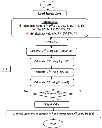
4.2. General algorithm

Figure 3 shows the general flow chart of the algorithm for SUPG-FEM.

Figure 3. Flow chart of algorithm

5. Results and discussion

In this article, the tilted slider-bearing parameters appear to be functions of the dimensionless parameters $P_e,P_r$, and E_c, as well as ${\gamma }^{⊛}$, ${\eta }^{⊛}$, w, A₁, b₁, Re, and ${\sigma }^{⊛}$. The following are the parameter values that were selected in accordance with the Lebeck consideration stated in Schumack(1996):

$U=20m/s,h_i=0.00005m,B=0.1m,c=1,926\text{break}J/kgK,T_a=310K,{\rho }_a=897.1kg/m3$, ${\mu }_a=0.0174\text{break}Pas,\beta =0.035K,\lambda =0.0012K,k=0.132W/(mK)$. The simulations were run for a range of values for the parameters $w,{\lambda }^{⊛},{\beta }^{⊛}$, and ${\sigma }^{⊛}$ with fixed values for P_e, P_r, and E_c. The roughness effect is only via, $h_o/3{\sigma }^{⊛}$, where, h_o, is the minimum film thickness as determined by Gururajan and Prakash (1999), can one experience the effects of roughness. When $ho\gg 3{\sigma }^{⊛}$, the effect of roughness is insignificant. However, if $ho\approx 3{\sigma }^{⊛}$ (within the HD limit, i.e. $h_o>3{\sigma }^{⊛}$), this could have a major impact on the bearing performance. For reasons of comparison, the parameter roughness of ${\sigma }^{⊛}$ is assumed to be fixed at 0.1, which is $25\mathrm{\%}$ and $10\mathrm{\%}$ of the minimum film thickness for w = 0.4 and w = 1.0, respectively. Furthermore, the constants ${\beta }^{⊛}=10$ and ${\lambda }^{⊛}=0.4$ are assumed to be fixed for the same.

The pressure distribution, load-bearing capacity, drag friction force, velocity, and temperature performance findings have been examined.

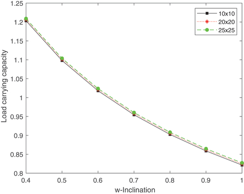
Tables and graphs are used to present the solutions. The numerical simulations were run on various grid systems with 10 by 10, 20 by 20, and 25 by 25 grid points to ensure grid independence at Re = 3000. Figure 4 compares and displays the load-carrying capacity performance of various grids. This leads to the conclusion that 25 by 25 yields a grid-independent solution. The conditions listed below have received special attention for turbulent fluid flow.

Condition(C1):	=	Thermal and surface roughness combined effect,
Condition(C2):	=	Effect of thermal on smooth surface,
Condition(C3):	=	Surface roughness effect for isothermal case.

Figure 4. Inclination vs load-carrying capacity on different grid system.

5.1. One-dimensional longitudinal surface roughness

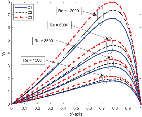
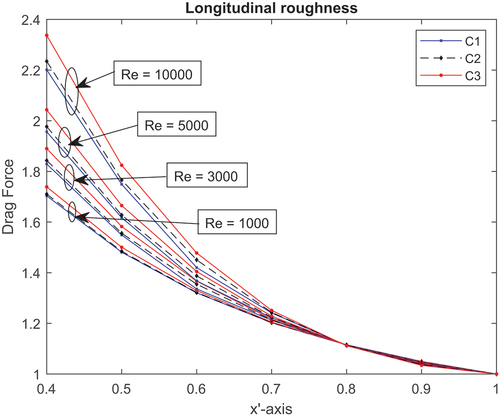
The one-dimensional longitudinal distribution of pressure performance brought on by the aforementioned conditions C₁, C₂ and C₃ for different local Reynolds numbers while taking turbulent fluid flow into consideration is shown in Figure 5. The load-carrying capacity performance (LCCP) for each fixed value of $x^{†}$ is in the order of conditions(C₁) < conditions(C₂) < conditions(C₃) for all circumstances. This indicates that as the local Reynolds numbers effect Re increased, the bearing’s LCCP increased. As a result, increasing the local Reynold numbers value causes pressure to rise and the flow of fluid to be obstructed. In contrast, surface roughness has a more significant impact than both the combined and the thermal effects. This highlights how crucial it is to consider surface roughness effects and local Reynolds numbers when estimating the load-carrying capability of slider bearings.

Figure 5. Pressure distributions at $T^i=T^p=T^s=1.0$, w = 0.4 and for different value of Re.

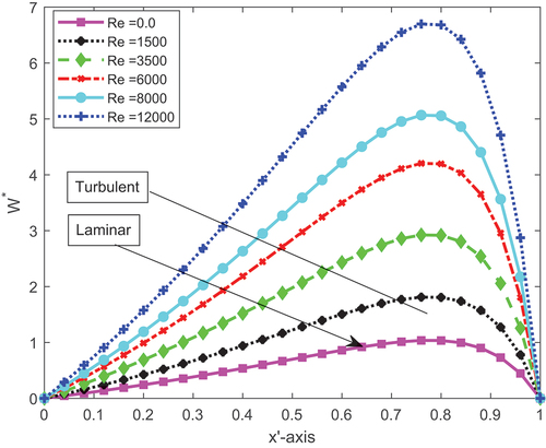
The pressure distribution of the longitudinal model type for turbulent and laminar fluid flow due to the local Reynolds number effect for non-parallel slider bearing, at the temperature of $T^i=T^p=T^s=1.0$, for condition (C₁) is shown in Figure 6. From this, it can be shown that the LCCP of the slider bearing grows as the local Reynolds number rises, and the LCCP of turbulent fluid flow is greater than laminar fluid flow. This result is in good agreement with Taylor (1969) and King and Taylor (1977).

Figure 6. Pressure distributions for turbulent and laminar flows for different Re.

The performance of LCCP and friction force of one-dimensional longitudinal surface roughness are shown for the aforementioned conditions and for various local Reynolds number values in Figures 7 and 8. It is clear that there is a reduction (16%) in LCCP for non-parallel (w = 0.4) between the surface roughness effect condition and the combined effect condition. Similar to this, for w = 0.4, there is a negligible, nearly 3%, decrease in friction force between C₁ and C₃ situations.

Figure 7. Pressure distributions at $T^i=T^p=T^s=1.0$, w = 0.4.

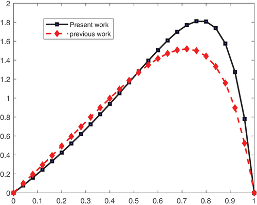
Figure 8. Longitudinal roughness LCCP vs inclination.

This is due to the fluid viscosity and density of the lubricant being reduced by the combined effect. As a result, the corresponding LCCP is reduced. Furthermore, there is a $3\mathrm{\%}$ difference in LCCP between C₁ and C₂, and no significant change in friction force is observed for non-parallel inclination.

In the case of the longitudinal roughness type, the texture is assumed to have the appearance of furrows, long narrow ridges, and valleys in the sliding direction (x-axis), which permits the fast flow of lubricant and results in a decrease in pressure distribution, which implies a reduction in the LCCP. Due to fluid expansion as the lubricant temperature rises, there is a load-carrying capacity generated in C₁ and C₂ in comparison to C₃ in the case of a parallel slider bearing at w = 1. Whereas there is no difference in LCCP between C₁ and C₂. This demonstrates the importance of taking into account turbulence terms and surface roughness effects when calculating the load-carrying capacity of slider-bearings. In addition, the peak of the pressure is noticed closer to the outlet, and the pattern of the graph of pressure distribution on the slider bearing is in good agreement with (Sinha & Adamu, 2009), (Kumar, 2001), (Rathish Kumar & Srinivasa Rao, 2000), (Desu Tessema et al., 2022), and (NB & Angadi, 2022). Figure 9 shows the pressure distribution for turbulent fluid flow of a slider bearing for local Reynolds number Re = 1000, which goes to laminar flow as given in the NG-Pan parameter of turbulent of Table 1, and the pressure distribution for laminar fluid flow, which is done in Desu Tessema et al. (2022), that indicate the present work is better than previous work. In general, our method has a better LCCP than other methods that appear in the literature.

Figure 9. Longitudinal roughness drag force vs inclination.

The surface plot of temperature for conditions C₁ and C₂ is shown in Figures 10 and 11. The temperature readings do not significantly vary, as shown by the two surface plot graphs.

Figure 10. Surface plot of temperature due to condition C₁ at w = 0.4 and $T^i=T^p=T^s=1.0$ (longitudinal roughness).

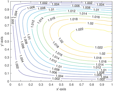
Figure 11. Surface plot of temperature due to condition C₂ at w = 0.4 and $T^i=T^p=T^s=1.0$ (longitudinal roughness).

According to Zienkiewicz (1957), a suction action may happen in parallel slider bearings if the pad bearing’s surface temperature is higher than the slider temperature. The study of the thermal impact on the slider and pad at a specific temperature of $(Ts<Tp$ or $Ts>Tp)$ on the LCCP and drag force of a sliding bearing is extremely relevant. Pinkus and Sternlicht (1961) state that in reality, the rest surface is usually warmer than the moving surface. The inlet lubricant temperature in a slider-bearing application being lower than the slider and pad temperatures is another crucial circumstance. Based on this, the combined effects of the following temperature boundary conditions on surface roughness and thermal conductivity have been examined for a range of local Reynolds numbers Re:

Case (i) :	=	$T^i=T^p=1.1and{T}^s=1.2,$
Case (ii):	=	$T^i=T^s=1.1and{T}^p=1.2,$
Case (iii):	=	$T^i=1.0,T^s=1.1and{T}^p=1.2,$
Case (iv):	=	$T^i=1.0,T^s=1.2and{T}^p=1.1$

The LCCP and drag force of one-dimensional longitudinal roughness are shown in Table 2 for different local Reynolds number effects corresponding to the mentioned cases. The slider and pad temperatures are lower or equal to the intake temperature.

Table 2. Longitudinal roughness $W^{⊛}$ and $F^{⊛}$ for condition (a) at different values of Re and w

Model	Re	w	0.4	0.6	0.8	1.0
i	Re = 1,000	$W^{⊛}$	0.2558	0.1185	0.0438	0.0046
		$F^{⊛}$	1.5796	1.2892	1.1154	0.9993
	Re = 3,000	$W^{⊛}$	0.4383	0.2037	0.0754	0.008
		$F^{⊛}$	1.6168	1.2978	1.1152	0.9988
	Re = 5,000	$W^{⊛}$	0.4096	0.2250	0.0878	0.0124
		$F^{⊛}$	1.6545	1.3065	1.115	0.9983
	Re = 8,000	$W^{⊛}$	0.5826	0.3200	0.1249	0.0177
		$F^{⊛}$	1.6989	1.3168	1.1147	0.9977
ii	Re = 1,000	$W^{⊛}$	0.2387	0.1309	0.0510	0.0072
		$F^{⊛}$	1.5759	1.2898	1.1152	1.001
	Re = 3,000	$W^{⊛}$	0.4096	0.2250	0.0878	0.0124
		$F^{⊛}$	1.6105	1.2988	1.1148	1.0017
	Re = 5,000	$W^{⊛}$	0.5826	0.3200	0.1249	0.0177
		$F^{⊛}$	1.6456	1.308	1.1144	1.0025
	Re = 8,000	$W^{⊛}$	0.7863	0.4322	0.1687	0.0239
		$F^{⊛}$	1.6868	1.3188	1.114	1.0033
iii	Re = 1,000	$W^{⊛}$	0.3838	0.2136	0.0877	0.0021
		$F^{⊛}$	1.6058	1.2982	1.1149	1.0003
	Re = 3,000	$W^{⊛}$	0.6582	0.3671	0.1508	0.0036
		$F^{⊛}$	1.6618	1.3134	1.1144	1.0006
	Re = 5,000	$W^{⊛}$	0.9362	0.5222	0.2146	0.0051
		$F^{⊛}$	1.7185	1.3287	1.1138	1.0008
	Re = 8,000	$W^{⊛}$	1.2633	0.7052	0.2898	0.0069
		$F^{⊛}$	1.7853	1.3468	1.1131	1.0011
iv	Re = 1,000	$W^{⊛}$	0.2909	0.1362	0.0505	0.0053
		$F^{⊛}$	1.5867	1.2909	1.1154	0.9993
	Re = 3,000	$W^{⊛}$	0.4983	0.2340	0.0869	0.0092
		$F^{⊛}$	1.6289	1.3007	1.1151	0.9987
	Re = 5,000	$W^{⊛}$	0.7088	0.3329	0.1236	0.0131
		$F^{⊛}$	1.6717	1.3107	1.1148	0.9982
	Re = 8,000	$W^{⊛}$	0.9562	0.4495	0.1670	0.0176
		$F^{⊛}$	1.7221	1.3224	1.1145	0.9975

When the temperature of the pad and slider is different, there is a 6% difference in LCCP between Case (ii) and Case (i) for w = 0.4 at Re = 1,000. For w = 1, Case (ii)’s LCCP is slightly better than Case (i)’s. In the case of drag force, there is no significant difference between Case (ii) and Case (i).

This table shows that if the inlet temperature is lower than that of the pad and slider, Case (iv)’s drag force of friction and LCCP are lower than Case (iii)’s for a non-parallel slider bearing. Accordingly, if the slider temperature is higher than the pad temperature, the temperature may drop due to turbulence and velocity applied to the slider effect, that increasing the LCCP and drag friction force.

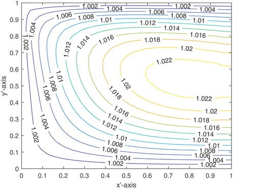
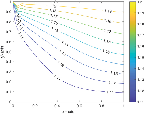
For a better understanding, Figures 12 and 13 depict the temperature contours of Cases (i) and Cases (ii) for w = 0.4. Due to Case (ii)’s greater average temperature than Case (i), Case (ii)’s LCCP is lower than Case (i)’s.

Figure 12. Contour line for Case (i) at w = 0.4 (longitudinal roughness).

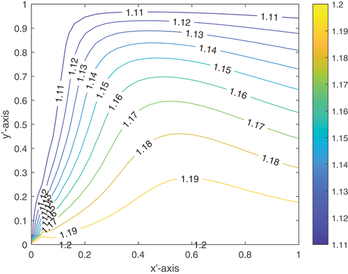
Figure 13. Contour line for Case (ii) at w = 0.4 (longitudinal roughness).

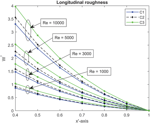
The performance of LCCP for different (${\delta }^{⊛}$) values is shown in Table 3 at a modified inertial value of (Re = 5,000). We can see from this table that as ${\delta }^{⊛}$ increases, the bearing’s LCCP decreases. This is because the surface roughness (asperity) increases, allowing for faster lubricant flow and a decrease in pressure distribution for the longitudinal roughness model; however, it is the opposite for the transversal roughness model. This is due to the fact that in the case of transverse roughness, the fluid is moving only in the x-direction and meets a series of constrictions at the flow gap (fluid film region) through which it must pass. This will hamper the flow and raise the LCCP of the slider bearing.

Table 3. Effect of surface roughness on LCCP for different values of σ^⊛, at w = 0.4, λ^⊛ = 0.4, Re^⊛ = 5,000, and β^⊛ = 10

$w^{⊛}$/${\sigma }^{⊛}$	0.0	0.02	0.04	0.06	0.08	0.10
Longitudinal	2.2573	2.2507	2.2311	2.1991	2.1560	2.1032
Transversal	2.3634	2.3838	2.4470	2.5586	2.7299	2.9825

5.2. U-velocity profile

Figure 14 depicts a plot of the one-dimensional longitudinal roughness U-velocity profile of the slider for case (iii) at x = 0.0, x = 0.24 and x = 0.48. One can observe from this that the velocity profile plot shows the stricture of sliders due to turbulent fluid lubrication flow at Re = 3,000. Figure 15 shows the contour plot of the U-velocity slider bearing for case (iii) at w = 0.4. Thus, the contour shows a zigzag form due to turbulence fluid flow at $Re=10,000$.

Figure 14. U-velocity profile for case (iii) for different x value at w = 0.4.

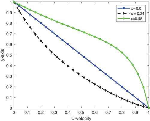
Figure 15. Contour plot of U-velocity profile for case (iii) at w = 0.4.

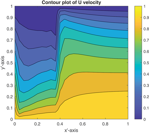
Table 4 shows the effect of U-velocity on bearing performance for condition(a) at w = 0.4 for different Re values and U-velocity. We can see from this table that as Re increases, the slider bearing’s LCCP and drag force increase. The reason for this is that when the local Reynolds number or turbulent lubrication effect rises, less lubricant can flow, which raises the pressure distribution and drag force for the longitudinal roughness model. However, contrary to this, as U-velocity increases, LCCP and drag force decrease. This is due to increasing u-velocity, which implies an increase in temperature that decreases the performance of LCCP and drag force slider bearings.

Table 4. Effect of U-Velocity on bearing performance for condition C₁ at w = 0.4 for different Re values

Re	$U/$	1.0	1.02	1.04	1.06	1.08	1.10
1,000	$W^{⊛}$	0.8626	0.8568	0.8511	0.8453	0.8395	0.8337
	$F^{⊛}$	1.7033	1.7022	1.7010	1.6998	1.6987	1.6975
3,000	$W^{⊛}$	1.4787	1.4688	1.4590	1.4490	1.4391	1.4291
	$F^{⊛}$	1.8291	1.8271	1.8251	1.8231	1.8211	1.8191
5,000	$W^{⊛}$	2.1032	2.0892	2.0751	2.0610	2.0468	2.0326
	$F^{⊛}$	1.9565	1.9537	1.9508	1.9480	1.9451	1.9422
8,000	$W^{⊛}$	2.8378	2.8189	2.7999	2.7809	2.7618	2.7426
	$F^{⊛}$	2.1064	2.1026	2.0988	2.0949	2.0910	2.0872
10,000	$W^{⊛}$	3.3020	3.2800	3.2579	3.2357	3.2135	3.1912
	$F^{⊛}$	2.2012	2.1967	2.1922	2.1878	2.1833	2.1788
12,000	$W^{⊛}$	3.7513	3.7264	3.7013	3.6761	3.6508	3.6255
	$F^{⊛}$	2.2929	2.2878	2.2827	2.2777	2.2725	2.2674

5.3. One-dimensional transverse roughness

Figure 16 shows a one-dimensional transverse roughness distribution of pressure performance resulting from the aforementioned conditions condition $(C_1,C_2$, and $C_3)$ for different local Reynolds number values. For any given value of $x^{†}$, the LCCP is in the condition sequence condition(C₂) < condition(C₁) < condition(C₃). This indicates that the LCCP of the bearing rose as the local Reynolds number effect did. Hence, a rise in the local Reynolds number and surface roughness causes a blockage in the fluid flow and an increase in pressure. Additionally, under all circumstances, surface roughness has a bigger impact than combined or thermal impacts overall, given the local Reynolds number. Figures 17 and 18 show the performance of LCCP and the friction force of one-dimensional transversal surface roughness for the aforementioned conditions and for different local Reynolds number values. It is clear that there is a reduction (33%) in LCCP for non-parallel (w = 0.4) between the surface roughness effect condition and the thermal effect condition. Similar to this, for w = 0.4, there is nearly 13% decrease in friction force between C₁ and C₃ situations. Moreover, for non-parallel inclination, the LCCP between C₁ and C₂ differs by $2\mathrm{\%}$, and a $3\mathrm{\%}$ change in drag frictional force is noted.

Figure 16. Transverse roughness pressure distributions at $T^i=T^p=T^s=1.0$ and w = 0.4.

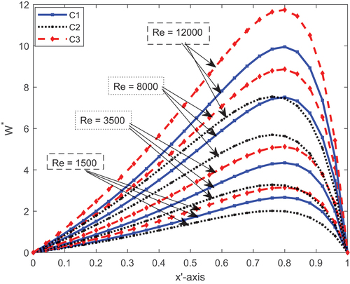
Figure 17. Transverse roughness LCCP vs inclination.

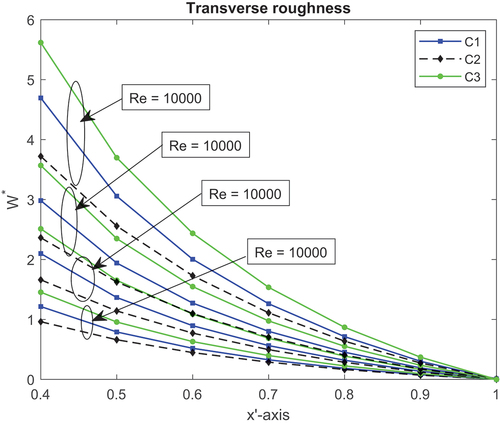
Figure 18. Transverse roughness drag force vs inclination.

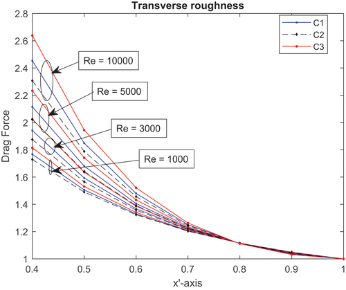
In general, in the case of transverse roughness, the fluid is moving only in the x-direction and meets a series of constrictions at the flow gap (fluid film region) through which it must pass. This will hamper the flow, besides the local Reynolds number effect due to turbulent fluid flow. On the other side, obstructing fluid flow and increasing pressure due to surface asperity valleys occurred. In relation to the pad and slider at different temperatures. Table 5 shows the same pecking order for pressure distribution and frictional force as the one-dimensional longitudinal distribution model, but with a slightly higher LCCP for a different local Reynolds number value Re. The results for drag force obtained for one-dimensional longitudinal roughness in cases (i)-(iv) are depicted in Table 5 and show almost identical patterns to those obtained for one-dimensional transverse roughness.

Table 5. Transverse roughness $W^{⊛}$ and $F^{⊛}$ for condition (a) at different values of Re and w

Model	Re	w	0.4	0.6	0.8	1.0
i	Re = 1,000	$W^{⊛}$	0.3705	0.1451	0.0507	0.0051
		$F^{⊛}$	1.6004	1.2918	1.1154	0.9992
	Re = 3,000	$W^{⊛}$	0.6399	0.2506	0.0876	0.0088
		$F^{⊛}$	1.6533	1.3024	1.1151	0.9987
	Re = 5,000	$W^{⊛}$	0.9091	0.3563	0.1246	0.0125
		$F^{⊛}$	1.7063	1.313	1.1149	0.9982
	Re = 8,000	$W^{⊛}$	1.229	0.4816	0.1684	0.0169
		$F^{⊛}$	1.7692	1.3256	1.1145	0.9975
ii	Re = 1,000	$W^{⊛}$	0.3232	0.1578	0.1036	0.0079
		$F^{⊛}$	1.5915	1.2924	1.1934	1.0011
	Re = 3,000	$W^{⊛}$	0.5581	0.2725	0.1023	0.0137
		$F^{⊛}$	1.638	1.3035	1.1147	1.0019
	Re = 5,000	$W^{⊛}$	0.7932	0.3874	0.1454	0.0195
		$F^{⊛}$	1.6846	1.3145	1.1142	1.0027
	Re = 8,000	$W^{⊛}$	1.0724	0.5237	0.1966	0.0263
		$F^{⊛}$	1.7398	1.3277	1.1137	1.0037
iii	Re = 1,000	$W^{⊛}$	0.528	0.2581	0.1015	0.0023
		$F^{⊛}$	1.6325	1.3026	1.1148	1.0004
	Re = 3,000	$W^{⊛}$	0.9119	0.4458	0.1752	0.0039
		$F^{⊛}$	1.7087	1.3212	1.1141	1.0006
	Re = 5,000	$W^{⊛}$	1.2958	0.6338	0.2491	0.0056
		$F^{⊛}$	1.7851	1.3397	1.1135	1.0009
	Re = 8,000	$W^{⊛}$	1.7519	0.8569	0.3368	0.0076
		$F^{⊛}$	1.8758	1.3618	1.1127	1.0012
iv	Re = 1,000	$W^{⊛}$	0.4199	0.1666	0.0584	0.0058
		$F^{⊛}$	1.6102	1.2938	1.1153	0.9992
	Re = 3,000	$W^{⊛}$	0.7252	0.2877	0.1009	0.0101
		$F^{⊛}$	1.6702	1.3059	1.115	0.9986
	Re = 5,000	$W^{⊛}$	1.0303	0.4089	0.1435	0.0144
		$F^{⊛}$	1.7303	1.3181	1.1147	0.9980
	Re = 8,000	$W^{⊛}$	1.3928	0.5529	0.1940	0.0194
		$F^{⊛}$	1.8017	1.3325	1.1143	0.9973

6. Conclusions

In this study, SUPG-FEM was used to demonstrate the turbulent fluid flow lubrication in slider bearings, together with the surface roughness and thermal effect. For one-dimensional transverse and longitudinal roughness types, bearing performance measurements including LCCP and drag frictional force were investigated. For the turbulent lubrication of the bearing, the modified turbulent lubrication equation was derived by applying the local film thickness under the actual surface profile to the Ng-Pan turbulent model. The following is a concise summary of the conclusions:

• In both types of models for non-parallel slider bearings, the achievement of the bearing performance (LCCP and drag force) improves. However, for w = 1 (parallel), the performance of bearing is negligible. The opposite is true for drag force in both model types.

• In the case of combined conditions, taking the temperature of the slider being higher than that of the pad, in both models, LCCP is higher for non-parallel bearing, whereas it goes to zero for parallel $(w=1)$.

• In all of the aforementioned conditions, the LCCP and drag force increase as the local Reynolds number of turbulence rises. This highlights the importance of considering the impacts of turbulent fluid flow and surface roughness.

• In general, a one-dimensional transversal model has a higher pressure distribution than a one-dimensional longitudinal roughness slider bearing.

The limitation of this proposed method is that it is difficult to apply a bilinear rectangular element for the discretization of the given irregular domain, especially in the slider bearing with irregular upper and lower boundaries. In the future, extend this method to bilinear triangular elements for the discretization of the domain.

Nomenclature

[A bar above a variable shows the expected value, whereas a superscript “$⊛$” indicates the non-dimensional quantity.]

List of symbol

1D	=	one dimensional
δ	=	random distribution of roughness
µ	=	viscosity of the lubricant
ρ	=	density of the lubricant
ρav	=	average density across the film
σ2	=	variation of roughness
B	=	bearing width
E	=	expected value operator
Ec	=	Eckert number
h	=	nominal film thickness
h0	=	nominal film thickness at outlet
hi	=	nominal film thickness at inlet
Ht	=	height of rough surface
k	=	thermal conductivity of lubricant
P	=	lubricant pressure
pe	=	Peclet number
pi	=	inlet pressure
pr	=	Prandtl number
T	=	lubricant temperature
Tav	=	average temperature across the film
U	=	velocity of the moving surface
v	=	velocity in the direction of the y-coordinate
w	=	$h_0/h_i$
$W^{⊛}$	=	load-carrying capacity of the bearing
$x^{†},y^{†}$	=	transformed coordinate system

Disclosure statement

No potential conflict of interest was reported by the author(s).

References

- Adamu, G., & Sinha, P. (2012). Thermal and roughness effects in a tilted pad slider bearing considering heat conduction through the pad and slider. Proceedings of the National Academy of Sciences, India Section A: Physical Sciences, 82(4), 323–333. https://doi.org/10.1007/s40010-012-0046-4
- Belhocine, A., & Abdullah, O. I. (2019). Numerical simulation of thermally developing turbulent flow through a cylindrical tube. The International Journal of Advanced Manufacturing Technology, 102(5–8), 2001–2012. https://doi.org/10.1007/s00170-019-03315-y
- Belhocine, A., & Afzal, A. (2022). Computational finite element analysis of brake disc rotors employing different materials. Australian Journal of Mechanical Engineering, 20(3), 637–650. https://doi.org/10.1080/14484846.2020.1733175
- Belhocine, A., & Omar, W. Z. W. (2017). Three-dimensional finite element modeling and analysis of the mechanical behavior of dry contact slipping between the disc and the brake pads. The International Journal of Advanced Manufacturing Technology, 88(1–4), 1035–1051. https://doi.org/10.1007/s00170-016-8822-y
- Belhocine, A., & Omar, W. Z. W. (2021). Analytical solution and numerical simulation of the generalized Levèque equation to predict the thermal boundary layer. Mathematics and Computers in Simulation, 180, 43–60. https://doi.org/10.1016/j.matcom.2020.08.007
- Belhocine, A., Stojanovic, N., & Abdullah, O. I. (2021). Numerical simulation of laminar boundary layer flow over a horizontal flat plate in external incompressible viscous fluid. European Journal of Computational Mechanics, 337–386. https://doi.org/10.13052/ejcm2642-2085.30463
- Belhocine, A., Stojanovic, N., & Abdullah, O. I. (2022). Numerical predictions of laminar flow and free convection heat transfer from an isothermal vertical flat plate. Archive of Mechanical Engineering, 69(4), 749–77. https://doi.org/10.24425/ame.2022.141523
- Black, H. (1970). Empirical treatment of hydrodynamic journal bearing performance in the superlaminar regime. Journal of Mechanical Engineering Science, 12(2), 116–122. https://doi.org/10.1243/JMES_JOUR_1970_012_019_02
- Brooks, A. N., & Hughes, T. J. (1982). Streamline upwind/Petrov–Galerkin formulations for convection dominated flows with particular emphasis on the incompressible Navier-Stokes equations. Computer Methods in Applied Mechanics and Engineering, 32(1–3), 199–259. https://doi.org/10.1016/0045-7825(82)90071-8
- Burton, R. (1974). Approximations in turbulent film analysis. Journal of Lubrication Technology, 96(1), 103–109. https://doi.org/10.1115/1.3451878
- Christensen, H. (1969). Stochastic models for hydrodynamic lubrication of rough surfaces. Proceedings of the Institution of Mechanical Engineers, 184(1), 1013–1026. https://doi.org/10.1243/PIME_PROC_1969_184_074_02
- Christensen, H., & Tonder, K. (1971). The hydrodynamic lubrication of rough bearing surfaces of finite width. Journal of Lubrication Technology, 93(3), 324–329. https://doi.org/10.1115/1.3451579
- Constantinescu, V. (1959). On turbulent lubrication. Proceedings of the Institution of Mechanical Engineers, 173(1), 881–900. https://doi.org/10.1243/PIME_PROC_1959_173_068_02
- Desu Tessema, G., Adamu Derese, G., Andargie Tiruneh, A., & Chen, X. (2022). Thermal and surface roughness effects on performance analysis of slider bearing via Petrov–Galerkin finite element method. Mathematical Problems in Engineering, 2022, 1–18. https://doi.org/10.1155/2022/4216136
- Ding, A., Dong Ren, X., Song Li, X., & Wei Gu, C. (2018). Numerical investigation of turbulence models for a superlaminar journal bearing. Advances in Tribology, 2018, 1–14. https://doi.org/10.1155/2018/2841303
- Elrod, H., Jr., & Ng, C. (1967). A theory for turbulent fluid films and its application to bearings. Journal of Lubrication Technology, 89(3), 346–362. https://doi.org/10.1115/1.3616989
- Guha, S. (2000). Analysis of steady-state characteristics of misaligned hydrodynamic journal bearings with isotropic roughness effect. Tribology International, 33(1), 1–12. https://doi.org/10.1016/S0301-679X(00)00005-0
- Gururajan, K., & Prakash, J. (1999). Surface roughness effects in infinitely long porous journal bearings. Journal of Tribology, 121(1), 139–147. https://doi.org/10.1115/1.2833795
- Hashimoto, H., & Wada, S. (1989). Theoretical approach to turbulent lubrication problems including surface roughness effects. Journal of Tribology, 111(1), 17–22. https://doi.org/10.1115/1.3261870
- Hirs, G. G. (1973). A bulk-flow theory for turbulence in lubricant films. Journal of Lubrication Technology, 95(2), 137–145. https://doi.org/10.1115/1.3451752
- Hooke, C. (1999). Fluid film lubrication: Theory and design (p. 414). 0521 48100 7. Cambridge University Press.
- Ho, M.-K., & Vohr, J. (1974). Application of energy model of turbulence to calculation of lubricant flows. Journal of Lubrication Technology, 96(1), 95–102. https://doi.org/10.1115/1.3451920
- King, K., & Taylor, C. (1977). An estimation of the effect of fluid inertia on the performance of the plane inclined slider thrust bearing with particular regard to turbulent lubrication. Journal of Lubrication Technology, 99(1), 129–135. https://doi.org/10.1115/1.3452961
- Kumar, B. R. (2001). A segregated supg/fem for thdl analysis in high speed slider bearings with injection effect. Journal of Tribology, 123(4), 732–741. https://doi.org/10.1115/1.1339980
- Lahmar, M., Bou-Saïd, B., & Tichy, J. (2013). The homogenization method of roughness analysis in turbulent lubrication. Proceedings of the Institution of Mechanical Engineers, Part J: Journal of Engineering Tribology, 227(10), 1090–1100. https://doi.org/10.1177/1350650113479844
- Lin, J.-R. (2000). Surface roughness effect on the dynamic stiffness and damping characteristics of compensated hydrostatic thrust bearings. International Journal of Machine Tools and Manufacture, 40(11), 1671–1689. https://doi.org/10.1016/S0890-6955(00)00012-2
- NB, N., & Angadi, A. (2022). On the dynamic characteristics of rough porous inclined slider bearing lubricated with micropolar fluid. Tribology Online, 17(1), 59–70. https://doi.org/10.2474/trol.17.59
- Ng, C.-W., & Pan, C. (1965). A linearized turbulent lubrication theory. Journal of Basic Engineering, 87(3), 675–682. https://doi.org/10.1115/1.3650640
- Pinkus, O., & Sternlicht, B. (1961). Theory of hydrodynamic lubrification. plus 0.5em minus 0.4em McGraw-Hill.
- Rathish Kumar, B., & Srinivasa Rao, P. (2000). Streamline upwind Petrov–Galerkin finite element analysis of thermal effects on load carrying capacity in slider bearings. Numerical Heat Transfer Part A-Applications, 38(3), 305–328. https://doi.org/10.1080/10407780050136549
- Schumack, M. (1996). Application of the pseudospectral method to thermohydrodynamic lubrication. International Journal for Numerical Methods in Fluids, 23(11), 1145–1161. https://doi.org/10.1002/(SICI)1097-0363(19961215)23:11<1145:AID-FLD459>3.0.CO;2-V
- Singh, D., Singh, N., & Awasthi, R. (2018). Effect of surface texture parameters on the performance of finite slider bearing. Materials Today: Proceedings, 5(9), 19349–19358. https://doi.org/10.1016/j.matpr.2018.06.294
- Sinha, P., & Adamu, G. (2009). Thd analysis for slider bearing with roughness: Special reference to load generation in parallel sliders. Acta Mechanica, 207(1–2), 11–27. https://doi.org/10.1007/s00707-008-0094-7
- Taylor, C. M. (1969). Paper 6: Turbulent lubrication theory applied to fluid film bearing design.
- Taylor, C., & Dowson, D. (1974). Turbulent lubrication theory-application to design.
- Wang, Y., Shan Liu, M., Qin, D., & Yan, Z. (2020). Performance of high-speed hydrodynamic sliding bearings with lubricating oils combining laminar and turbulent flows. Advances in Mechanical Engineering, 12(6), 168781402093338. https://doi.org/10.1177/1687814020933389
- Zhang, Z.-M., Wang, X.-J., & Sun, M.-L. (2003). Turbulence models of hydrodynamic lubrication. Journal of Shanghai University (English Edition), 7(4), 305–314. https://doi.org/10.1007/s11741-003-0001-3
- Zhu, S., Sun, J., Li, B., Zhao, X., Wang, H., Teng, Q., Ren, Y., & Zhu, G. (2019). Stochastic models for turbulent lubrication of bearing with rough surfaces. Tribology International, 136, 224–233. https://doi.org/10.1016/j.triboint.2019.03.063
- Zienkiewicz, O. (1957). Temperature distribution within lubricating films between parallel bearing surfaces and its effect on the pressures developed. Proceedings the Conference on Lubrication and Wear, 135. https://cir.nii.ac.jp/crid/1572543024553290624