Uniform persistence and backward bifurcation of vertically transmitted vector-borne diseases

ABSTRACT

Vertical transmissions of vector-borne diseases such as dengue virus, malaria, West Nile virus and Rift Valley fever are among challenging factors in disease control. In this paper, we used a system of differential equations to study the impacts of vertical transmission (in the vector) and horizontal (vector-to-host) transmissions cycle on the uniform persistence of a vertically transmitted disease. This is given analytically when the secondary reproduction number is greater than unity. Additional numerical results indicate that vertical transmission rates raise the epidemic level. However, we provide analytical results to reveal that vertical transmission of the disease in vectors alone without horizontal transmission, could not make the disease endemic. Furthermore, by transforming the system of differential equations to a nonlinear eigenvalue equation, the existence of a backward bifurcation is established. The directions of bifurcation is forward when the disease-induced death rate of hosts is reduced below a threshold. It is shown that the bifurcation is backward when the disease-induced death rate in the host is above a critical value. Additionally, increased disease transmission parameters also contribute to backward bifurcation. Numerical results are also provided to highlight that, depending on the initial conditions, the disease could be persistent even when the secondary reproduction number is less than unity.

KEYWORDS:

• vertical transmission
• uniform persistence
• backward bifurcation
• vector-borne

MATHEMATICS SUBJECT CLASSIFICATION:

• 92D30
• 92B05
• 37G99

View correction statement:

Correction

1. Introduction

Vector-borne diseases such as malaria, dengue virus, West Nile virus, Rift-Valley fever and yellow fever are among major public health problems that claim the lives of human beings and domestic animals. These diseases also cause economic challenges in the world, mostly in developing countries. Additionally, the geographic distributions of some of these vector-borne diseases overlap with the developed world, including many parts of the United States (Centers for Disease Control and Prevention) and Europe (Hubálek & Halouzka, 1999). Furthermore, many vector-borne diseases are recurring and becoming endemic in some parts of the world owing to deteriorating environmental conditions due to human activities. Some of these are deforestation, poorly managed irrigation systems, dams, and other factors connected to climate variations which influence physiological changes in mosquitoes

Major disease vectors, such as Anophelis, Aedes aegypti and Aedes albopictus mosquito species transmit dengue virus (Adams & Boots, 2010; Feng & Velasco-Hernández, 1997), West Nile virus (Blayneh et al., 2010; Cruz-Pacheco et al., 2009; Pu et al., 2023), and Rift Valley fever (Chitnis et al., 2013; Gaff et al., 2007) to humans and domestic animals. These mosquito species also pass the disease causing pathogen to their eggs which contributes to vertical transmission. The survival of some exposed eggs through the winter season is believed to enable the emerging adult mosquitoes to continue with the transmission cycle once conditions are favorable (Adams & Boots, 2010).

Vertical transmission of yellow fever is believed to be the cause for overwintering of the disease keeping transmission cycle in Amazon (Francisco, 2007). However, although vertical transmission enhances seasonal outbreak of diseases, it alone, could not be enough to make the disease endemic without vector-to-host (also known as horizontal) transmission cycle. Therefore, a more significant challenge comes from the presence of a horizontal transmission. Moreover, according to studies of mosquito-borne diseases, the most effective fights against horizontal transmission encompass mosquito control and personal protections (Blayneh, 2017; Blayneh et al., 2009, 2010; Gordillo, 2013). It is clear that several efforts are employed to control mosquitoes, such as releasing sterile mosquito population (Zheng, 2022) and effects of larva predators (Zhu et al., 2023). The existence of a backward bifurcation phenomena is one indicator that control efforts could fail, because of existence of endemic equilibrium points for secondary reproductive number reduced below one. Contributions to the phenomena of backward bifurcation come from a combination of several factors, primarily, poor personal protections and also fatality of the diseases (Blayneh, 2017; Blayneh et al., 2010; Chitnis et al., 2006; Dushoff et al., 1998). Disease transmissions within the host in addition to horizontal (vector-host) transmission cycle could add more challenges to the dynamic of a vector-borne disease, see for example the work of (Wang et al., 2020), where the analysis explores age of infection. Our work focuses on a vertically transmitted disease within the vector population, the effects of vertical transmission rate on disease prevalence and other factors which contribute to the persistence of the vector-borne disease.

Persistence of diseases contributes to challenges against control efforts. A biological system exhibits the phenomena of persistence when a solution which is initially positive (componentwise) has no compartment that dies out in the long run (Allen, 2007). This means, no boundary equilibrium is the omega limit set of any solution with initial condition in the positive cone. Several articles have investigated the dynamics of biological systems reflecting different forms of persistence. Some focus on models describing ecological systems, such as Lotka-Volterra type applied to food-chain (see (Allen, 2007) and references therein) and predator-prey (Allen, 2007; Joseph et al., 1986). Likewise, the persistence of epidemics problems has been addressed by few authors. Among them, we have (Thieme, 2001) on uniform weak-persistence of diseases, Robelo (Robelo et al., 2014) on persistence of diseases in a periodic environment. Similarly, the uniform persistence of diseases are modeled by some authors, notable examples include van den Driessche and Yakubu on discrete-time model (van den Driessche & Yakubu, 2019), Gourley et al. (2014) on bluetongue dynamic and (Salako, 2023) on the impact of population size and movement on two-strain infectious diseases. Clearly, uniform persistence is strong enough to guarantee that any solution with positive initial value remains bounded away from the boundary equilibrium.

The objectives of this work are to prove the existence of a backward bifurcation when the disease-induced death rate in the host population is above a critical value, mosquito population equilibrates to a large number and personal protections are poor; to establish the uniform persistence of vertically transmitted vector-borne diseases and also, to prove that vertical transmission in the vector alone does not cause the disease to be endemic without vector-to-host transmission cycle. These results are established using the model studied in (Blayneh, 2017). Specifically, the important roll played by vector-to-host transmission cycle to establish the disease as endemic is proved in Section (3). Furthermore, the existence of a backward bifurcation is established in Section (4). The uniform persistence of the disease, when the secondary reproduction number is greater than unity, is proved in Section (5). This implies that despite the initial value, each compartment of the disease approaches a positive quantity. Our results highlight the importance of reducing the epidemiology threshold (secondary reproduction number) below unity and factors which cause this effort to fail. Additionally, in the presence of a backward bifurcation, depending on the initial values, the disease could equilibrate to an endemic level for some ${\mathcal{R}}_0$ less than unity. This is supported by numerical results presented in Section (5). Discussion and concluding remarks are given in Section (6).

2. The model for vector-host transmission cycle

The model studied in (Blayneh, 2017) is extended to address very important problems emerging from vertically transmitted vector-borne diseases, where the vertical transmission takes place in the vector population. First, we present some background steps which lead to the main model. To this end, we use $x_1,x_2,x_3$ and x₄ to describe the number of hosts which are susceptible, exposed, infectious, and recovered, respectively. Similarly, $y_1,y_2$ and y₃ represent the number of susceptible, exposed and infectious vectors, respectively. Furthermore, $N=\sum _{i=1}^4{x}_i\mathrm{and}P=\sum _{i=1}^3{y}_i,$ denote the total population sizes of the host and vector, respectively.

As it is given in (Blayneh, 2017), the inflow of exposed mosquitoes (also known as vectors) comes from transmission of the disease through bites of susceptible mosquitoes (on exposed or infectious) hosts and also, adults emerging from eggs laid by infectious mosquitoes. More specifically, susceptible mosquitoes become exposed to the disease by a bite from exposed and infectious hosts with transmission efficacy θ₁ and ${\theta }_2,$ respectively. Thus, the forces of infection for a susceptible vector due to a bite of exposed host is $\frac{\varphi {\theta }_1{x}_2}{N},$ and due to a bite of infectious host is $\frac{\varphi {\theta }_2{x}_3}{N},$ where ϕ is the number of bites that a host sustains per unit time. Therefore, the number of exposed mosquitoes due to horizontal (vector-host) transmission per unit time is $(\frac{\varphi {\theta }_1{x}_2}{N}+\frac{\varphi {\theta }_2{x}_3}{N})y_1.$ Additional inflow of exposed mosquitoes comes from vertical transmission given by ${\delta }_1\zeta y_3,$ where ζ is the rate of disease transmission from a female mosquito to eggs per unit time and δ₁ is the proportion of eggs reaching to adult stage. Thus, the inflow of exposed mosquitoes is $(\frac{\varphi {\theta }_1{x}_3}{N}+\frac{\varphi {\theta }_2{x}_2}{N})y_1+{\delta }_1\zeta y_3.$ The average number of mosquito recruitment is δ₀ and this quantity is increased by a proportion of eggs from susceptible and exposed mosquitoes reaching to adult stage, plus eggs from infectious mosquitoes which became susceptible adults, which is ${\delta }_1(1-\zeta )y_3$. Thus, the susceptible mosquito population increases by ${\delta }_0+{\delta }_1(y_1+y_2)+{\delta }_1(1-\zeta )y_3$ per unit time, which implies $\frac{d{y}_1}{dt}={\delta }_0+{\delta }_1(y_1+y_2)+{\delta }_1(1-\zeta )y_3-(\frac{\varphi {\theta }_1{x}_3}{N}+\frac{\varphi {\theta }_2{x}_2}{N})y_1-\gamma y_1.$

The change in exposed mosquito population is $\frac{d{y}_2}{dt}=\frac{\varphi {\theta }_1{x}_3{y}_1}{N}+\frac{\varphi {\theta }_2{x}_2{y}_1}{N}+{\delta }_1\zeta y_3-\phi y_2-\gamma y_2.$ It should be noted that the rate of disease progression in mosquito is $\phi ,$ and γ is the natural death rate of vectors. The inflow of exposed hosts is given by $\frac{\varphi \beta y_3{x}_1}{N}$ and the rate of progress from exposed to infectious level in the host is $d,$ which is also known as an incubation rate of the disease in a host per unit time. Thus, $\frac{d{x}_2}{dt}=\frac{\beta \varphi y_3{x}_1}{N}-d{x}_2-\mu x_2,$ where µ is natural mortality rate of hosts. Infectious hosts have three ways to exit the compartment: by recovery at a rate of $r,$ by natural death at a rate of µ or due to disease-induced death rate which is $\alpha .$ Based on these facts, the rate of change in $x_3,$ infectious hosts is$\frac{d{x}_3}{dt}=d{x}_2-(r+\alpha +\mu )x_3.$ Furthermore, a recovered host becomes susceptible to the disease at a rate of $\psi .$ Incoming host population to the community is assumed to be susceptible. Since the disease is not vertically transmitted in the host population, all new borne hosts are susceptible. These results are the bases for the system of differential equation model given by the system in model (1(1) $\begin{array}{ll}\frac{d{x}_1}{dt}& =\rho +\mathrm{\Lambda }N+\psi x_4-\frac{\beta \varphi y_3{x}_1}{N}-\mu x_1\\ \frac{d{x}_2}{dt}& =\frac{\beta \varphi y_3{x}_1}{N}-d{x}_2-\mu x_2\\ \frac{d{x}_3}{dt}& =d{x}_2-(r+\alpha +\mu )x_3\\ \frac{d{x}_4}{dt}& =r{x}_3-(\psi +\mu )x_4\\ \frac{d{y}_1}{dt}& ={\delta }_0+{\delta }_1(y_1+y_2)+{\delta }_1(1-\zeta )y_3-\frac{\varphi {\theta }_1{x}_3{y}_1}{N}\\ -\frac{\varphi {\theta }_2{x}_2{y}_1}{N}-\gamma y_1\\ \frac{d{y}_2}{dt}& =\frac{\varphi {\theta }_1{x}_3{y}_1}{N}+\frac{\varphi {\theta }_2{x}_2{y}_1}{N}+{\delta }_1\zeta y_3-\phi y_2-\gamma y_2\\ \frac{d{y}_3}{dt}& =\phi y_2-\gamma y_3,\end{array}$(1) ). For the description of all parameters refer to (Table 1).

(1) $\begin{array}{ll}\frac{d{x}_1}{dt}& =\rho +\mathrm{\Lambda }N+\psi x_4-\frac{\beta \varphi y_3{x}_1}{N}-\mu x_1\\ \frac{d{x}_2}{dt}& =\frac{\beta \varphi y_3{x}_1}{N}-d{x}_2-\mu x_2\\ \frac{d{x}_3}{dt}& =d{x}_2-(r+\alpha +\mu )x_3\\ \frac{d{x}_4}{dt}& =r{x}_3-(\psi +\mu )x_4\\ \frac{d{y}_1}{dt}& ={\delta }_0+{\delta }_1(y_1+y_2)+{\delta }_1(1-\zeta )y_3-\frac{\varphi {\theta }_1{x}_3{y}_1}{N}\\ -\frac{\varphi {\theta }_2{x}_2{y}_1}{N}-\gamma y_1\\ \frac{d{y}_2}{dt}& =\frac{\varphi {\theta }_1{x}_3{y}_1}{N}+\frac{\varphi {\theta }_2{x}_2{y}_1}{N}+{\delta }_1\zeta y_3-\phi y_2-\gamma y_2\\ \frac{d{y}_3}{dt}& =\phi y_2-\gamma y_3,\end{array}$(1)

Table 1. Model parameter and their descriptions

Parameter	Description (rates are per day)
µ	natural mortality rate of hosts
ζ	vertical disease transmission rate from female mosquito to egg
δ0	average number of new adult female mosquitoes
δ1	a factor for density dependent maturation to adulthood
Λ	per capita birth rate of hosts
r	recovery rate of hosts
β	the probability of disease transmission from infectious vector to susceptible host
	from an infected vector to a susceptible host
ρ	immigration rate of susceptible hosts
ϕ	the number of bites a host sustains from a mosquito(host-vector contact rate)
α	disease-induced host death rate
ψ	fading rate of treatment to make hosts susceptible to the disease
γ	mortality rate of vectors
φ	incubation rate of the disease in a vector
d	incubation rate of the disease in a host
θ1	probability of disease transmission from infectious host to vector
θ2	probability of disease transmission from exposed host to vector

Next, with $X=(x_1,x_2,x_3,x_4)$ and $Y=(y_1,y_2,y_3),$ we define the set

(2) $\begin{array}{ll}\mathrm{\Omega }=& \{(X,Y)\in R_{+}^4\times R_{+}^3,\sum _{i=1}^4{x}_i\in [0,\frac{\rho }{\mu -\mathrm{\Lambda }}],\\ \sum _{i=1}^3{y}_i\in [0,\frac{{\delta }_0}{\gamma -{\delta }_1}]\}\\ =& \{X\in R_{+}^4,\sum _{i=1}^4{x}_i\in [0,\frac{\rho }{\mu -\mathrm{\Lambda }}]\}\times \\ \{Y\in R_{+}^3,\sum _{i=1}^3{y}_i\in [0,\frac{{\delta }_0}{\gamma -{\delta }_1}]\}\end{array}$(2)

which is biologically feasible and forward invariant under system (1(1) $\begin{array}{ll}\frac{d{x}_1}{dt}& =\rho +\mathrm{\Lambda }N+\psi x_4-\frac{\beta \varphi y_3{x}_1}{N}-\mu x_1\\ \frac{d{x}_2}{dt}& =\frac{\beta \varphi y_3{x}_1}{N}-d{x}_2-\mu x_2\\ \frac{d{x}_3}{dt}& =d{x}_2-(r+\alpha +\mu )x_3\\ \frac{d{x}_4}{dt}& =r{x}_3-(\psi +\mu )x_4\\ \frac{d{y}_1}{dt}& ={\delta }_0+{\delta }_1(y_1+y_2)+{\delta }_1(1-\zeta )y_3-\frac{\varphi {\theta }_1{x}_3{y}_1}{N}\\ -\frac{\varphi {\theta }_2{x}_2{y}_1}{N}-\gamma y_1\\ \frac{d{y}_2}{dt}& =\frac{\varphi {\theta }_1{x}_3{y}_1}{N}+\frac{\varphi {\theta }_2{x}_2{y}_1}{N}+{\delta }_1\zeta y_3-\phi y_2-\gamma y_2\\ \frac{d{y}_3}{dt}& =\phi y_2-\gamma y_3,\end{array}$(1) ). Specifically, if (X, Y) is a solution of system (1(1) $\begin{array}{ll}\frac{d{x}_1}{dt}& =\rho +\mathrm{\Lambda }N+\psi x_4-\frac{\beta \varphi y_3{x}_1}{N}-\mu x_1\\ \frac{d{x}_2}{dt}& =\frac{\beta \varphi y_3{x}_1}{N}-d{x}_2-\mu x_2\\ \frac{d{x}_3}{dt}& =d{x}_2-(r+\alpha +\mu )x_3\\ \frac{d{x}_4}{dt}& =r{x}_3-(\psi +\mu )x_4\\ \frac{d{y}_1}{dt}& ={\delta }_0+{\delta }_1(y_1+y_2)+{\delta }_1(1-\zeta )y_3-\frac{\varphi {\theta }_1{x}_3{y}_1}{N}\\ -\frac{\varphi {\theta }_2{x}_2{y}_1}{N}-\gamma y_1\\ \frac{d{y}_2}{dt}& =\frac{\varphi {\theta }_1{x}_3{y}_1}{N}+\frac{\varphi {\theta }_2{x}_2{y}_1}{N}+{\delta }_1\zeta y_3-\phi y_2-\gamma y_2\\ \frac{d{y}_3}{dt}& =\phi y_2-\gamma y_3,\end{array}$(1) ) with nonnegative initial values $(X(0),Y(0)),$ where $0\le \sum _{i=1}^4{x}_i(0)\le \frac{\rho }{\mu -\mathrm{\Lambda }}$ and $0\le \sum _{i=1}^3{y}_i(0)\le \frac{{\delta }_0}{\gamma -{\delta }_1},$ then $\sum _{i=1}^4{x}_i(t)\in [0,\frac{\rho }{\mu -\mathrm{\Lambda }}]$ and $\sum _{i=1}^3{y}_i(t)\in [0,\frac{{\delta }_0}{\gamma -{\delta }_1}]$ and furthermore, the total population size is eventually attracted to this set (Blayneh, 2017).

The disease-free equilibrium of (1(1) $\begin{array}{ll}\frac{d{x}_1}{dt}& =\rho +\mathrm{\Lambda }N+\psi x_4-\frac{\beta \varphi y_3{x}_1}{N}-\mu x_1\\ \frac{d{x}_2}{dt}& =\frac{\beta \varphi y_3{x}_1}{N}-d{x}_2-\mu x_2\\ \frac{d{x}_3}{dt}& =d{x}_2-(r+\alpha +\mu )x_3\\ \frac{d{x}_4}{dt}& =r{x}_3-(\psi +\mu )x_4\\ \frac{d{y}_1}{dt}& ={\delta }_0+{\delta }_1(y_1+y_2)+{\delta }_1(1-\zeta )y_3-\frac{\varphi {\theta }_1{x}_3{y}_1}{N}\\ -\frac{\varphi {\theta }_2{x}_2{y}_1}{N}-\gamma y_1\\ \frac{d{y}_2}{dt}& =\frac{\varphi {\theta }_1{x}_3{y}_1}{N}+\frac{\varphi {\theta }_2{x}_2{y}_1}{N}+{\delta }_1\zeta y_3-\phi y_2-\gamma y_2\\ \frac{d{y}_3}{dt}& =\phi y_2-\gamma y_3,\end{array}$(1) ) is

(3) $E_0=(x_1^{\ast },0,0,0,y_1^{\ast },0,0),$(3)

where $x_1^{\ast }=\frac{\rho }{\mu -\mathrm{\Lambda }}$, $y_1^{\ast }=\frac{{\delta }_0}{\gamma -{\delta }_1}.$ This is obtained by setting the disease-related variables to zero: $x_2=x_3=x_4=y_2=y_3=0,$ then solving for x₁ and y₁ from the equilibrium equation of System (1(1) $\begin{array}{ll}\frac{d{x}_1}{dt}& =\rho +\mathrm{\Lambda }N+\psi x_4-\frac{\beta \varphi y_3{x}_1}{N}-\mu x_1\\ \frac{d{x}_2}{dt}& =\frac{\beta \varphi y_3{x}_1}{N}-d{x}_2-\mu x_2\\ \frac{d{x}_3}{dt}& =d{x}_2-(r+\alpha +\mu )x_3\\ \frac{d{x}_4}{dt}& =r{x}_3-(\psi +\mu )x_4\\ \frac{d{y}_1}{dt}& ={\delta }_0+{\delta }_1(y_1+y_2)+{\delta }_1(1-\zeta )y_3-\frac{\varphi {\theta }_1{x}_3{y}_1}{N}\\ -\frac{\varphi {\theta }_2{x}_2{y}_1}{N}-\gamma y_1\\ \frac{d{y}_2}{dt}& =\frac{\varphi {\theta }_1{x}_3{y}_1}{N}+\frac{\varphi {\theta }_2{x}_2{y}_1}{N}+{\delta }_1\zeta y_3-\phi y_2-\gamma y_2\\ \frac{d{y}_3}{dt}& =\phi y_2-\gamma y_3,\end{array}$(1) ). For the sake of simplifying notations, we introduce $k_i,i=1,\dots ,4.$

(4) $k_1=d+\mu ,k_2=\psi +\mu ,k_3=r+\alpha +\mu ,k_4=\phi +\gamma .$(4)

A1: $\gamma >{\delta }_1,$ $\mu >\mathrm{\Lambda }$ and $\zeta \in [0,1).$

The secondary reproduction number which is obtained using the approaches in (van den Driessche & Watmough, 2002) is

(5) ${\mathcal{R}}_0={\mathcal{R}}_0(\zeta )=\frac{\zeta {\delta }_1\phi }{2\gamma k_4}+\sqrt{{\left(\frac{\zeta {\delta }_1\phi }{2\gamma k_4}\right)}^2+{\mathcal{R}}_h^2},$(5)

where

(6) ${\mathcal{R}}_h=\varphi \sqrt{\frac{\beta \phi ({\theta }_{1}d+{\theta }_2{k}_3)y_1^{\ast }}{k_1{k}_3{k}_4\gamma x_1^{\ast }}}.$(6)

The theory of next-generation matrix provided by (van den Driessche & Watmough, 2002), states that the secondary reproduction number ${\mathcal{R}}_0$ is $\rho (F{V}^{-1}),$ the spectral radius of $F{V}^{-1}.$ F is the Jacobian of new infection function $(\frac{\beta \varphi y_3{x}_1}{N},0,0,\frac{\varphi {\theta }_1{x}_3{y}_1}{N}+\frac{\varphi {\theta }_1{x}_3{y}_1}{N}+\frac{\varphi {\theta }_2{x}_2{y}_1}{N}+{\delta }_1\zeta y_3,0)$ it is proved that the disease-free equilibrium point $E_0,$ given by (3(3) $E_0=(x_1^{\ast },0,0,0,y_1^{\ast },0,0),$(3) ), of system (1(1) $\begin{array}{ll}\frac{d{x}_1}{dt}& =\rho +\mathrm{\Lambda }N+\psi x_4-\frac{\beta \varphi y_3{x}_1}{N}-\mu x_1\\ \frac{d{x}_2}{dt}& =\frac{\beta \varphi y_3{x}_1}{N}-d{x}_2-\mu x_2\\ \frac{d{x}_3}{dt}& =d{x}_2-(r+\alpha +\mu )x_3\\ \frac{d{x}_4}{dt}& =r{x}_3-(\psi +\mu )x_4\\ \frac{d{y}_1}{dt}& ={\delta }_0+{\delta }_1(y_1+y_2)+{\delta }_1(1-\zeta )y_3-\frac{\varphi {\theta }_1{x}_3{y}_1}{N}\\ -\frac{\varphi {\theta }_2{x}_2{y}_1}{N}-\gamma y_1\\ \frac{d{y}_2}{dt}& =\frac{\varphi {\theta }_1{x}_3{y}_1}{N}+\frac{\varphi {\theta }_2{x}_2{y}_1}{N}+{\delta }_1\zeta y_3-\phi y_2-\gamma y_2\\ \frac{d{y}_3}{dt}& =\phi y_2-\gamma y_3,\end{array}$(1) ) is locally asymptotically stable if ${\mathcal{R}}_0<1$ and unstable if ${\mathcal{R}}_0>1,$ where ${\mathcal{R}}_0$ is defined by (5(5) ${\mathcal{R}}_0={\mathcal{R}}_0(\zeta )=\frac{\zeta {\delta }_1\phi }{2\gamma k_4}+\sqrt{{\left(\frac{\zeta {\delta }_1\phi }{2\gamma k_4}\right)}^2+{\mathcal{R}}_h^2},$(5) ) (see (Blayneh, 2017)).

In Section 4, we present some conditions under which the disease equilibrate to endemic level even if ${\mathcal{R}}_0<1.$ Next, we look into the limitations of vertical transmissions and the importance of horizontal transmission to magnify the dynamic a vertically transmitted vector-borne disease.

3. Can vertical transmission sustain the virus without a horizontal transmission?

Vector-host contact is the base for a horizontal transmission of any vector-borne disease. In vertically transmitted vector-borne diseases, additional transmission occurs due to mosquitoes passing the disease to eggs, which could become infectious adults maintaining the transmission cycle within the mosquito population. The goal of this section is to show that vertical transmission alone can not support the persistence of the disease in the absence of interactions with hosts (no horizontal transmission). A host could be human or animal where female mosquitoes get blood meal. We begin our study by assuming that the host population is susceptible, but there are infectious mosquitoes supporting vertical transmission with no opportunity to pass the disease to hosts. To see this, consider the system (1(1) $\begin{array}{ll}\frac{d{x}_1}{dt}& =\rho +\mathrm{\Lambda }N+\psi x_4-\frac{\beta \varphi y_3{x}_1}{N}-\mu x_1\\ \frac{d{x}_2}{dt}& =\frac{\beta \varphi y_3{x}_1}{N}-d{x}_2-\mu x_2\\ \frac{d{x}_3}{dt}& =d{x}_2-(r+\alpha +\mu )x_3\\ \frac{d{x}_4}{dt}& =r{x}_3-(\psi +\mu )x_4\\ \frac{d{y}_1}{dt}& ={\delta }_0+{\delta }_1(y_1+y_2)+{\delta }_1(1-\zeta )y_3-\frac{\varphi {\theta }_1{x}_3{y}_1}{N}\\ -\frac{\varphi {\theta }_2{x}_2{y}_1}{N}-\gamma y_1\\ \frac{d{y}_2}{dt}& =\frac{\varphi {\theta }_1{x}_3{y}_1}{N}+\frac{\varphi {\theta }_2{x}_2{y}_1}{N}+{\delta }_1\zeta y_3-\phi y_2-\gamma y_2\\ \frac{d{y}_3}{dt}& =\phi y_2-\gamma y_3,\end{array}$(1) ) with $\beta =\varphi ={\theta }_1={\theta }_2=0.$ In the absence of horizontal transmission, all of the terms describing disease transmission from infectious hosts to susceptible mosquitoes are eliminated from fifth equation in system (1(1) $\begin{array}{ll}\frac{d{x}_1}{dt}& =\rho +\mathrm{\Lambda }N+\psi x_4-\frac{\beta \varphi y_3{x}_1}{N}-\mu x_1\\ \frac{d{x}_2}{dt}& =\frac{\beta \varphi y_3{x}_1}{N}-d{x}_2-\mu x_2\\ \frac{d{x}_3}{dt}& =d{x}_2-(r+\alpha +\mu )x_3\\ \frac{d{x}_4}{dt}& =r{x}_3-(\psi +\mu )x_4\\ \frac{d{y}_1}{dt}& ={\delta }_0+{\delta }_1(y_1+y_2)+{\delta }_1(1-\zeta )y_3-\frac{\varphi {\theta }_1{x}_3{y}_1}{N}\\ -\frac{\varphi {\theta }_2{x}_2{y}_1}{N}-\gamma y_1\\ \frac{d{y}_2}{dt}& =\frac{\varphi {\theta }_1{x}_3{y}_1}{N}+\frac{\varphi {\theta }_2{x}_2{y}_1}{N}+{\delta }_1\zeta y_3-\phi y_2-\gamma y_2\\ \frac{d{y}_3}{dt}& =\phi y_2-\gamma y_3,\end{array}$(1) ) Furthermore, since the focus is on the disease dynamics in the mosquito population, without contribution of disease from infectious hosts, we consider only the last three equations of the system, which are

(7) $\begin{array}{ll}\frac{d{y}_1}{dt}& ={\delta }_0+{\delta }_1(y_1+y_2)+{\delta }_1(1-\zeta )y_3-\gamma y_1\\ \frac{d{y}_2}{dt}& ={\delta }_1\zeta y_3-(\phi +\gamma )y_2\\ \frac{d{y}_3}{dt}& =\phi y_2-\gamma y_3.\end{array}$(7)

It should be noted that the parameters and variables used in (7(7) $\begin{array}{ll}\frac{d{y}_1}{dt}& ={\delta }_0+{\delta }_1(y_1+y_2)+{\delta }_1(1-\zeta )y_3-\gamma y_1\\ \frac{d{y}_2}{dt}& ={\delta }_1\zeta y_3-(\phi +\gamma )y_2\\ \frac{d{y}_3}{dt}& =\phi y_2-\gamma y_3.\end{array}$(7) ) are the same as those in (1(1) $\begin{array}{ll}\frac{d{x}_1}{dt}& =\rho +\mathrm{\Lambda }N+\psi x_4-\frac{\beta \varphi y_3{x}_1}{N}-\mu x_1\\ \frac{d{x}_2}{dt}& =\frac{\beta \varphi y_3{x}_1}{N}-d{x}_2-\mu x_2\\ \frac{d{x}_3}{dt}& =d{x}_2-(r+\alpha +\mu )x_3\\ \frac{d{x}_4}{dt}& =r{x}_3-(\psi +\mu )x_4\\ \frac{d{y}_1}{dt}& ={\delta }_0+{\delta }_1(y_1+y_2)+{\delta }_1(1-\zeta )y_3-\frac{\varphi {\theta }_1{x}_3{y}_1}{N}\\ -\frac{\varphi {\theta }_2{x}_2{y}_1}{N}-\gamma y_1\\ \frac{d{y}_2}{dt}& =\frac{\varphi {\theta }_1{x}_3{y}_1}{N}+\frac{\varphi {\theta }_2{x}_2{y}_1}{N}+{\delta }_1\zeta y_3-\phi y_2-\gamma y_2\\ \frac{d{y}_3}{dt}& =\phi y_2-\gamma y_3,\end{array}$(1) ). Accordingly, the only flow of exposed mosquitoes comes from $\delta \zeta y_3$ which is exposed adults from eggs of infectious mosquito. Exposed vectors develop the disease to be infectious at a rate of $\phi .$ Mortality rate of mosquitoes per unit time is $\gamma .$ Clearly, (7(7) $\begin{array}{ll}\frac{d{y}_1}{dt}& ={\delta }_0+{\delta }_1(y_1+y_2)+{\delta }_1(1-\zeta )y_3-\gamma y_1\\ \frac{d{y}_2}{dt}& ={\delta }_1\zeta y_3-(\phi +\gamma )y_2\\ \frac{d{y}_3}{dt}& =\phi y_2-\gamma y_3.\end{array}$(7) ) is a linear system, and the last two equations do not involve $y_1.$ Therefore, we first consider the subsystem

(8) $\begin{array}{ll}\frac{d{y}_2}{dt}& ={\delta }_1\zeta y_3-(\phi +\gamma )y_2\\ \frac{d{y}_3}{dt}& =\phi y_2-\gamma y_3.\end{array}$(8)

The coefficient matrix of this subsystem is

(9) $\mathcal{A}=\left(\begin{array}{ll}-(\phi +\gamma )& {\delta }_1\zeta \\ \phi & -\gamma \end{array}\right).$(9)

The trace of $\mathcal{A}<0$ and the determinant of $\mathcal{A}$ is $\gamma (\phi +\gamma )-\phi \zeta {\delta }_1>0$, because $0\le \zeta <1$ and ${\delta }_1<\gamma .$ This implies that the eigenvalues of $\mathcal{A}$ have negative real parts. Thus, the unique equilibrium $(y_2,y_3)=(0,0)$ of the subsystem (8(8) $\begin{array}{ll}\frac{d{y}_2}{dt}& ={\delta }_1\zeta y_3-(\phi +\gamma )y_2\\ \frac{d{y}_3}{dt}& =\phi y_2-\gamma y_3.\end{array}$(8) ) is globally asymptotically stable. Suppose $(y_1(t),y_2(t),y_3(t))$ is a solution of (7(7) $\begin{array}{ll}\frac{d{y}_1}{dt}& ={\delta }_0+{\delta }_1(y_1+y_2)+{\delta }_1(1-\zeta )y_3-\gamma y_1\\ \frac{d{y}_2}{dt}& ={\delta }_1\zeta y_3-(\phi +\gamma )y_2\\ \frac{d{y}_3}{dt}& =\phi y_2-\gamma y_3.\end{array}$(7) ) with positive initial conditions $(y_1(0),y_2(0),y_3(0)).$ It is clear that the first equation in (7(7) $\begin{array}{ll}\frac{d{y}_1}{dt}& ={\delta }_0+{\delta }_1(y_1+y_2)+{\delta }_1(1-\zeta )y_3-\gamma y_1\\ \frac{d{y}_2}{dt}& ={\delta }_1\zeta y_3-(\phi +\gamma )y_2\\ \frac{d{y}_3}{dt}& =\phi y_2-\gamma y_3.\end{array}$(7) ) is equivalent to

(10) $\frac{d{y}_1}{dt}+(\gamma -{\delta }_1)y_1={\delta }_0+{\delta }_1{y}_2++{\delta }_1(1-\zeta )y_3.$(10)

Using integrating factor $e^{(\gamma -{\delta }_1)t},$ we write the solution with initial condition $y_1(0),$ as

(11) $y_1(t)=\frac{{\delta }_0}{\gamma -{\delta }_1}+y_1(0)e^{-(\gamma -{\delta }_1)t}-\frac{{\delta }_0{e}^{-(\gamma -{\delta }_1)t}}{\gamma -{\delta }_1}+{\delta }_1{\int }_0^{t}B(s)ds,$(11)

where

(12) $\begin{array}{ll}B(s)& =(y_2(s)+(1-\zeta )y_3(s))e^{(\gamma -{\delta }_1)(s-t)}.\end{array}$(12)

Furthermore, $\underset{t\to \mathrm{\infty }}{lim sup}\mid y_2(t)+(1-\zeta )y_3(t)\mid =0.$ Thus, the last term in (11(11) $y_1(t)=\frac{{\delta }_0}{\gamma -{\delta }_1}+y_1(0)e^{-(\gamma -{\delta }_1)t}-\frac{{\delta }_0{e}^{-(\gamma -{\delta }_1)t}}{\gamma -{\delta }_1}+{\delta }_1{\int }_0^{t}B(s)ds,$(11) ) satisfies the following condition

(13) $\begin{array}{l}0\le \mid {\int }_0^t(y_2(s)+(1-\zeta )y_3(s))e^{(\gamma -{\delta }_1)(s-t)}ds\mid \le \\ \frac{{\delta }_1}{\gamma -{\delta }_1}(1-e^{-(\gamma -{\delta }_1)t})\underset{t\to \mathrm{\infty }}{lim sup}\mid y_2(t)+(1-\zeta )y_3(t)\mid =0.\end{array}$(13)

Therefore, $y_1(t)$ given by (11(11) $y_1(t)=\frac{{\delta }_0}{\gamma -{\delta }_1}+y_1(0)e^{-(\gamma -{\delta }_1)t}-\frac{{\delta }_0{e}^{-(\gamma -{\delta }_1)t}}{\gamma -{\delta }_1}+{\delta }_1{\int }_0^{t}B(s)ds,$(11) ) approaches $\frac{{\delta }_0}{\gamma -{\delta }_1}.$ Since $(y_2,y_3)$ approaches $(0,0),$ we conclude that the equilibrium of system (7(7) $\begin{array}{ll}\frac{d{y}_1}{dt}& ={\delta }_0+{\delta }_1(y_1+y_2)+{\delta }_1(1-\zeta )y_3-\gamma y_1\\ \frac{d{y}_2}{dt}& ={\delta }_1\zeta y_3-(\phi +\gamma )y_2\\ \frac{d{y}_3}{dt}& =\phi y_2-\gamma y_3.\end{array}$(7) ), $(\frac{{\delta }_0}{\gamma -{\delta }_1},0,0),$ is globally asymptotically stable. The conclusion from this result is that according to our model, vertical transmission alone does not sustain the disease. Some studies support the importance of epidemic circulation to make a disease endemic (see Adams & Boots (2010) and references therein). Clearly, since the disease is vertically transmitted from mosquito to egg, some surviving infected eggs could become infectious adults. However, this may not be significant enough to produce more infectious adults which could sustain the number of infectious mosquitoes in the environment. Epidemic circulation in an environment, which is primarily supported by vector-host transmission cycle could establish the disease as endemic. On the other hand, many factors such as rainfall and temperature affect the physiology of mosquitoes. The contribution of these factors could amplify the effects of vertical transmission on the prevalence of the disease.

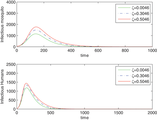
(Figure 1) shows how vertical transmission amplifies disease prevalence.

Figure 1. A time plot reflecting the effects of vertical transmission in the vector population on disease prevalence: ζ = 0.0046 (continuous/green curve), ζ = 0.3046 (dashed/blue curve) and ζ = 0.5046 (continuous/red curve). Other parameters are $\alpha =0.0065$, $\gamma =1/17$, $\beta =0.15,{\theta }_1=0.0083,{\theta }_2=0.0072$, $\mu =3.91\times {10}^{-5},\text{upLambda}=1.48\times {10}^{-5},\rho =205,{\delta }_0=1150,r=1/7,{\delta }_1=0.0397,d=1/6,\psi =0.00243,\varphi =2.$ For each case ${\mathcal{R}}_0<1$.

4. Backward bifurcation and possible causes

In this section, we establish the existence of a backward bifurcation phenomena. Our approach is by building an operator equation for the exposed groups in the host and the vector populations. Then, we define a bifurcation parameter where the critical value of this parameter corresponds to ${\mathcal{R}}_0=1.$ We proved that the operator has a geometrically simple characteristic eigenvalue. Then, we use a theorem given in (Cushing, 1998) to conclude the existence of a bifurcating branch at the critical point. Similar approaches are used in (Chitnis et al., 2006, 2013). The bifurcation result given in (Blayneh, 2017) involves complex parameter combination, because of which it was not possible to highlight on the disease-induced death rate and related parameters describing disease transmission cycles. Our approach in this work clears that there is no backward bifurcation when the disease-induce death rate is reduced below a threshold level. Additionally, horizontal transmission cycle and the steady state level of mosquitoes play a role in the emergence of a backward bifurcation when the disease-induce death rate is increased. To begin, let $E=(x_1,x_2,x_3,x_4,y_1,y_2,y_3)$ be an endemic equilibrium of System (1(1) $\begin{array}{ll}\frac{d{x}_1}{dt}& =\rho +\mathrm{\Lambda }N+\psi x_4-\frac{\beta \varphi y_3{x}_1}{N}-\mu x_1\\ \frac{d{x}_2}{dt}& =\frac{\beta \varphi y_3{x}_1}{N}-d{x}_2-\mu x_2\\ \frac{d{x}_3}{dt}& =d{x}_2-(r+\alpha +\mu )x_3\\ \frac{d{x}_4}{dt}& =r{x}_3-(\psi +\mu )x_4\\ \frac{d{y}_1}{dt}& ={\delta }_0+{\delta }_1(y_1+y_2)+{\delta }_1(1-\zeta )y_3-\frac{\varphi {\theta }_1{x}_3{y}_1}{N}\\ -\frac{\varphi {\theta }_2{x}_2{y}_1}{N}-\gamma y_1\\ \frac{d{y}_2}{dt}& =\frac{\varphi {\theta }_1{x}_3{y}_1}{N}+\frac{\varphi {\theta }_2{x}_2{y}_1}{N}+{\delta }_1\zeta y_3-\phi y_2-\gamma y_2\\ \frac{d{y}_3}{dt}& =\phi y_2-\gamma y_3,\end{array}$(1) ), then close to the disease-free equilibrium $E_0=(x_1^{\ast },0,0,0,y_1^{\ast },0,0),$ x₂ and y₂ satisfy the following equations

(14) $\begin{array}{ll}{x}_2=& \frac{\varphi \beta \phi }{\gamma k_1}{y}_2+\frac{\varphi \beta \phi }{\gamma k_1}[\frac{{\mathcal{H}}_1}{\rho k_2{k}_3}+\frac{d\alpha }{\rho k_3}]x_2{y}_2\\ y_2=& \frac{{\mathcal{H}}_2{\delta }_0\gamma (\mu -\mathrm{\Lambda })}{\rho (\gamma k_4-{\delta }_1\zeta \phi )}{x}_2+\frac{d\alpha {\mathcal{H}}_2(\mu -\mathrm{\Lambda }){\delta }_0\gamma }{k_3{\rho }^2(\gamma k_4-{\delta }_1\zeta \phi )}{x}_2^2\\ -\frac{(\gamma -{\delta }_1)k_4{\mathcal{H}}_2(\mu -\mathrm{\Lambda })}{\rho (\gamma k_4-{\delta }_1\zeta \phi )}{x}_2{y}_2,\end{array}$(14)

where

(15) $\begin{array}{ll}{\mathcal{H}}_1=& \psi rd-k_1{k}_2{k}_3+\mathrm{\Lambda }(k_2{k}_3+rd+r{k}_2)\text{and}\\ {\mathcal{H}}_2=& \frac{\varphi ({\theta }_{1}d+{\theta }_2{k}_3)}{k_3(\gamma -{\delta }_1)}.\end{array}$(15)

Note that assumption (A1) in Section (2) implies that the term $\gamma k_4-{\delta }_1\zeta \phi >0.$ Next, select a bifurcation parameter

(16) $\mathrm{\Delta }=\frac{\beta \varphi {\delta }_0(\mu -\mathrm{\Lambda })}{\rho (\gamma -{\delta }_1)}=\frac{\beta \varphi y_1^{\ast }}{x_1^{\ast }},$(16)

and using $\mathrm{\Delta },$ transform Equation (14)(14) $\begin{array}{ll}{x}_2=& \frac{\varphi \beta \phi }{\gamma k_1}{y}_2+\frac{\varphi \beta \phi }{\gamma k_1}[\frac{{\mathcal{H}}_1}{\rho k_2{k}_3}+\frac{d\alpha }{\rho k_3}]x_2{y}_2\\ y_2=& \frac{{\mathcal{H}}_2{\delta }_0\gamma (\mu -\mathrm{\Lambda })}{\rho (\gamma k_4-{\delta }_1\zeta \phi )}{x}_2+\frac{d\alpha {\mathcal{H}}_2(\mu -\mathrm{\Lambda }){\delta }_0\gamma }{k_3{\rho }^2(\gamma k_4-{\delta }_1\zeta \phi )}{x}_2^2\\ -\frac{(\gamma -{\delta }_1)k_4{\mathcal{H}}_2(\mu -\mathrm{\Lambda })}{\rho (\gamma k_4-{\delta }_1\zeta \phi )}{x}_2{y}_2,\end{array}$(14) to

(17) $\begin{array}{ll}{x}_2& =\frac{\mathrm{\Delta }\phi x_1^{\ast }}{\gamma k_1{y}_1^{\ast }}{y}_2+\frac{\mathrm{\Delta }\phi x_1^{\ast }}{\gamma k_1{k}_2{k}_3{y}_1^{\ast }}({\mathcal{H}}_1+d\alpha k_2)x_2{y}_2\\ y_2& =\frac{\mathrm{\Delta }({\theta }_{1}d+{\theta }_2{k}_3)\gamma }{\beta k_3(\gamma k_4-{\delta }_1\zeta \phi )}[x_2+\frac{d\alpha }{\rho k_3}{x}_2^2-\frac{k_4}{y_1^{\ast }\gamma }{x}_2{y}_2].\end{array}$(17)

Then the nonlinear eigenvalue equation becomes

(18) $x=\mathrm{\Delta }\mathcal{L}x+h(\mathrm{\Delta },x),$(18)

where

(19) $\mathcal{L}=\left(\begin{array}{ll}0& \frac{\phi x_1^{\ast }}{\gamma k_1{y}_1^{\ast }}\\ \frac{({\theta }_{1}d+{\theta }_2{k}_3)\gamma }{\beta k_3(\gamma k_4-{\delta }_1\zeta \phi )}& 0\end{array}\right),$(19)

(20) $\begin{array}{ll}h(\mathrm{\Delta },x)=& \left(\begin{array}{l}\frac{\mathrm{\Delta }\phi x_1^{\ast }}{\gamma \rho k_1{k}_2{k}_3{y}_1^{\ast }}({\mathcal{H}}_1+d\alpha k_2)x_2{y}_2\\ \frac{\mathrm{\Delta }({\theta }_{1}d+{\theta }_2{k}_3)\gamma }{\beta k_3^2(\gamma k_4-{\delta }_1\zeta \phi )}[\frac{\alpha d}{\rho }{x}_2^2-\frac{k_4{k}_3}{\gamma y_1^{\ast }}{x}_2{y}_2]\end{array}\right)\text{and}\\ x=& \left(\begin{array}{l}{x}_2\\ y_2\end{array}\right).\end{array}$(20)

To apply known bifurcation theorem and pull fundamental results, we first need to lay preliminary steps. To this end, the set $R_{+}^2=\{(x_2,y_2),x_2>0,y_2>0\}$ is a Banach space under the Euclidean norm. The boundary $\partial R_{+}^2$ carries vectors where at least one component is zero. System (1(1) $\begin{array}{ll}\frac{d{x}_1}{dt}& =\rho +\mathrm{\Lambda }N+\psi x_4-\frac{\beta \varphi y_3{x}_1}{N}-\mu x_1\\ \frac{d{x}_2}{dt}& =\frac{\beta \varphi y_3{x}_1}{N}-d{x}_2-\mu x_2\\ \frac{d{x}_3}{dt}& =d{x}_2-(r+\alpha +\mu )x_3\\ \frac{d{x}_4}{dt}& =r{x}_3-(\psi +\mu )x_4\\ \frac{d{y}_1}{dt}& ={\delta }_0+{\delta }_1(y_1+y_2)+{\delta }_1(1-\zeta )y_3-\frac{\varphi {\theta }_1{x}_3{y}_1}{N}\\ -\frac{\varphi {\theta }_2{x}_2{y}_1}{N}-\gamma y_1\\ \frac{d{y}_2}{dt}& =\frac{\varphi {\theta }_1{x}_3{y}_1}{N}+\frac{\varphi {\theta }_2{x}_2{y}_1}{N}+{\delta }_1\zeta y_3-\phi y_2-\gamma y_2\\ \frac{d{y}_3}{dt}& =\phi y_2-\gamma y_3,\end{array}$(1) ) has only one disease-free equilibrium, therefore, $x=(0,0)$ is unique on $\partial R_{+}^2.$ Furthermore, $\mathcal{L}:R_{+}^2\to R_{+}^2$ is a compact operator. This follows from the fact that for any bounded subset $\mathcal{D}$ of $R_{+}^2$, $\mathcal{L}(\mathcal{D})$ lies in a compact subset of $R_{+}^2.$ For an open interval $\mathrm{\Theta }\subset R,$ we define

(21) $\mathrm{\Sigma }=\mathrm{\Theta }\times R_{+}^2$(21)

and verify the existence of a continuum $C^{+}\subset \mathrm{\Sigma }$ which bifurcates from a critical point $({\mathrm{\Delta }}_0,0),$ where

(22) ${\mathrm{\Delta }}_0=\sqrt{\frac{\beta y_1^{\ast }{k}_1{k}_3(\gamma k_4-{\delta }_1\zeta \phi )}{x_1^{\ast }\phi ({\theta }_{1}d+{\theta }_2{k}_3)}}$(22)

Here, a pair $(\mathrm{\Delta },x)$ on $C^{+}$ represents a solution x of (18(18) $x=\mathrm{\Delta }\mathcal{L}x+h(\mathrm{\Delta },x),$(18) ) corresponding to $\mathrm{\Delta },$ where $x=(x_2,y_2{)}^{\tau },$ (τ is transpose) is a component of an endemic equilibrium $E=(x_1,x_2,x_3,x_4,y_1,y_2,y_3)$ for system (1(1) $\begin{array}{ll}\frac{d{x}_1}{dt}& =\rho +\mathrm{\Lambda }N+\psi x_4-\frac{\beta \varphi y_3{x}_1}{N}-\mu x_1\\ \frac{d{x}_2}{dt}& =\frac{\beta \varphi y_3{x}_1}{N}-d{x}_2-\mu x_2\\ \frac{d{x}_3}{dt}& =d{x}_2-(r+\alpha +\mu )x_3\\ \frac{d{x}_4}{dt}& =r{x}_3-(\psi +\mu )x_4\\ \frac{d{y}_1}{dt}& ={\delta }_0+{\delta }_1(y_1+y_2)+{\delta }_1(1-\zeta )y_3-\frac{\varphi {\theta }_1{x}_3{y}_1}{N}\\ -\frac{\varphi {\theta }_2{x}_2{y}_1}{N}-\gamma y_1\\ \frac{d{y}_2}{dt}& =\frac{\varphi {\theta }_1{x}_3{y}_1}{N}+\frac{\varphi {\theta }_2{x}_2{y}_1}{N}+{\delta }_1\zeta y_3-\phi y_2-\gamma y_2\\ \frac{d{y}_3}{dt}& =\phi y_2-\gamma y_3,\end{array}$(1) ) which is connected to (14(14) $\begin{array}{ll}{x}_2=& \frac{\varphi \beta \phi }{\gamma k_1}{y}_2+\frac{\varphi \beta \phi }{\gamma k_1}[\frac{{\mathcal{H}}_1}{\rho k_2{k}_3}+\frac{d\alpha }{\rho k_3}]x_2{y}_2\\ y_2=& \frac{{\mathcal{H}}_2{\delta }_0\gamma (\mu -\mathrm{\Lambda })}{\rho (\gamma k_4-{\delta }_1\zeta \phi )}{x}_2+\frac{d\alpha {\mathcal{H}}_2(\mu -\mathrm{\Lambda }){\delta }_0\gamma }{k_3{\rho }^2(\gamma k_4-{\delta }_1\zeta \phi )}{x}_2^2\\ -\frac{(\gamma -{\delta }_1)k_4{\mathcal{H}}_2(\mu -\mathrm{\Lambda })}{\rho (\gamma k_4-{\delta }_1\zeta \phi )}{x}_2{y}_2,\end{array}$(14) ). It is clear that the remaining components of E can be solved from the equilibrium equation. Specifically, for $(x_2,y_2)$ on the bifurcating curve for (14(14) $\begin{array}{ll}{x}_2=& \frac{\varphi \beta \phi }{\gamma k_1}{y}_2+\frac{\varphi \beta \phi }{\gamma k_1}[\frac{{\mathcal{H}}_1}{\rho k_2{k}_3}+\frac{d\alpha }{\rho k_3}]x_2{y}_2\\ y_2=& \frac{{\mathcal{H}}_2{\delta }_0\gamma (\mu -\mathrm{\Lambda })}{\rho (\gamma k_4-{\delta }_1\zeta \phi )}{x}_2+\frac{d\alpha {\mathcal{H}}_2(\mu -\mathrm{\Lambda }){\delta }_0\gamma }{k_3{\rho }^2(\gamma k_4-{\delta }_1\zeta \phi )}{x}_2^2\\ -\frac{(\gamma -{\delta }_1)k_4{\mathcal{H}}_2(\mu -\mathrm{\Lambda })}{\rho (\gamma k_4-{\delta }_1\zeta \phi )}{x}_2{y}_2,\end{array}$(14) ), we go to system (1(1) $\begin{array}{ll}\frac{d{x}_1}{dt}& =\rho +\mathrm{\Lambda }N+\psi x_4-\frac{\beta \varphi y_3{x}_1}{N}-\mu x_1\\ \frac{d{x}_2}{dt}& =\frac{\beta \varphi y_3{x}_1}{N}-d{x}_2-\mu x_2\\ \frac{d{x}_3}{dt}& =d{x}_2-(r+\alpha +\mu )x_3\\ \frac{d{x}_4}{dt}& =r{x}_3-(\psi +\mu )x_4\\ \frac{d{y}_1}{dt}& ={\delta }_0+{\delta }_1(y_1+y_2)+{\delta }_1(1-\zeta )y_3-\frac{\varphi {\theta }_1{x}_3{y}_1}{N}\\ -\frac{\varphi {\theta }_2{x}_2{y}_1}{N}-\gamma y_1\\ \frac{d{y}_2}{dt}& =\frac{\varphi {\theta }_1{x}_3{y}_1}{N}+\frac{\varphi {\theta }_2{x}_2{y}_1}{N}+{\delta }_1\zeta y_3-\phi y_2-\gamma y_2\\ \frac{d{y}_3}{dt}& =\phi y_2-\gamma y_3,\end{array}$(1) ) and solve for x₃ from the third equation, then for x₄ from the fourth equation. Also, adding the fifth and sixth equations, we solve for $y_1.$ Similarly we solve for $y_1,$ adding the first and the second equations. It should be noted that in the presence of a backward bifurcation, there are two endemic equilibrium points for ${\mathcal{R}}_0<1.$

We now proceed to establish the existence of a continuum $C^{+}\subset \mathrm{\Sigma }$ of solutions of (18(18) $x=\mathrm{\Delta }\mathcal{L}x+h(\mathrm{\Delta },x),$(18) ) and identify bifurcation points for Equation (18)(18) $x=\mathrm{\Delta }\mathcal{L}x+h(\mathrm{\Delta },x),$(18) . This is provided in the following lemma.

Lemma 4.1.

The nonlinear eigenvalue equation given by (18(18) $x=\mathrm{\Delta }\mathcal{L}x+h(\mathrm{\Delta },x),$(18) ) has a continuum $C^{+}\subset \mathrm{\Sigma }$, where $(\mathrm{\Delta },x)\in C^{+}-\{({\mathrm{\Delta }}_0,0)\}$ is a solution pair of (18(18) $x=\mathrm{\Delta }\mathcal{L}x+h(\mathrm{\Delta },x),$(18) ), where Δ₀ is defined by (22(22) ${\mathrm{\Delta }}_0=\sqrt{\frac{\beta y_1^{\ast }{k}_1{k}_3(\gamma k_4-{\delta }_1\zeta \phi )}{x_1^{\ast }\phi ({\theta }_{1}d+{\theta }_2{k}_3)}}$(22) ) and $x=(x_2,y_2).$ $C^{+}$ bifurcates at $({\mathrm{\Delta }}_0,0),$ where $\mathrm{\Delta }={\mathrm{\Delta }}_0$ if and only if ${\mathcal{R}}_0=1.$

Proof.

First, the eigenvalues of $\mathcal{L}$ are ${\lambda }_{+}=\sqrt{\frac{x_1^{\ast }\phi ({\theta }_{1}d+{\theta }_2{k}_3)}{\beta y_1^{\ast }{k}_1{k}_3(\gamma k_4-{\delta }_1\zeta \phi )}}$ and ${\lambda }_{-}=-\sqrt{\frac{x_1^{\ast }\phi ({\theta }_{1}d+{\theta }_2{k}_3)}{\beta y_1^{\ast }{k}_1{k}_3(\gamma k_4-{\delta }_1\zeta \phi )}}.$

Let

(23) $a_{12}=\frac{\phi x_1^{\ast }}{\gamma k_1{y}_1^{\ast }},a_{21}=\frac{({\theta }_{1}d+{\theta }_2{k}_3)\gamma }{\beta k_3(\gamma k_4-{\delta }_1\zeta \phi )},$(23)

and using these new notations we have ${\lambda }_{+}=\sqrt{a_{12}{a}_{21}}$ and ${\lambda }_{-}=-\sqrt{a_{12}{a}_{21}}.$ Clearly, ${\lambda }_{+}$ and ${\lambda }_{-}$ are algebraically simple and nonzero. This implies that

(24) ${\mathrm{\Delta }}_0=\frac{1}{{\lambda }_{+}}=1/\sqrt{a_{12}{a}_{21}}$(24)

and ${\mathrm{\Delta }}_{01}=\frac{1}{{\lambda }_{-}}=-1/\sqrt{a_{12}{a}_{21}}$ are characteristic values of $\mathcal{L}.$ Corresponding to ${\mathrm{\Delta }}_0,$ the right characteristic vector of $\mathcal{L}$ is ${\mathrm{\Delta }}_0(\sqrt{a_{12}{a}_{21}},a_{21}{)}^{\tau },\text{and}{\mathrm{\Delta }}_0(a_{21},\sqrt{a_{12}{a}_{21}})$ is the left characteristic vector. However, it should be noted that the characteristic vector corresponding to Δ₀₁ is $(1,\frac{-\sqrt{a_{12}{a}_{21}}}{a_{21}})$ and it is not positive componentwise.

According to Rabinowitz (1971) and Cushing (1998), the eigenvalue problem given by (18(18) $x=\mathrm{\Delta }\mathcal{L}x+h(\mathrm{\Delta },x),$(18) ) has a continuum of nontrivial solutions, $(\mathrm{\Delta },x),$ of (17(17) $\begin{array}{ll}{x}_2& =\frac{\mathrm{\Delta }\phi x_1^{\ast }}{\gamma k_1{y}_1^{\ast }}{y}_2+\frac{\mathrm{\Delta }\phi x_1^{\ast }}{\gamma k_1{k}_2{k}_3{y}_1^{\ast }}({\mathcal{H}}_1+d\alpha k_2)x_2{y}_2\\ y_2& =\frac{\mathrm{\Delta }({\theta }_{1}d+{\theta }_2{k}_3)\gamma }{\beta k_3(\gamma k_4-{\delta }_1\zeta \phi )}[x_2+\frac{d\alpha }{\rho k_3}{x}_2^2-\frac{k_4}{y_1^{\ast }\gamma }{x}_2{y}_2].\end{array}$(17) ) one which bifurcates from $({\mathrm{\Delta }}_0,0)$ and the other from $({\mathrm{\Delta }}_{01},0)$. Since the left and right characteristic vectors corresponding to Δ₀ are both positive componentwise, the continuum bifurcating from $({\mathrm{\Delta }}_0,0)$, which we denote by $C^{+}$ is positive, but the other continuum bifurcating from $({\mathrm{\Delta }}_{01},0)$ is not positive. Furthermore, since there is no other critical point different from $({\mathrm{\Delta }}_0,0)$ and $({\mathrm{\Delta }}_{01},0),$ the branch $C^{+}$ remains in the positive quadrant.

Finally, we show that $\mathrm{\Delta }={\mathrm{\Delta }}_0$ is equivalent to ${\mathcal{R}}_0=1.$ To see this, observe that $\mathrm{\Delta }={\mathrm{\Delta }}_0$ implies $\frac{\beta \varphi y_1^{\ast }}{x_1^{\ast }}=\sqrt{\frac{\beta k_1{k}_3(\gamma k_4-{\delta }_1\zeta \phi )y_1^{\ast }}{({\theta }_{1}d+{\theta }_2{k}_3)x_1^{\ast }}},$ then squaring both sides and simplifying terms we get $\frac{{\varphi }^2\beta \phi ({\theta }_{1}d+{\theta }_2{k}_3)y_1^{\ast }}{\gamma k_1{k}_3{k}_4{x}_1^{\ast }}=1-\frac{{\delta }_1\zeta \phi }{\gamma k_4}.$ The left side of this equation is ${\mathcal{R}}_h^2,$ which is given by (6(6) ${\mathcal{R}}_h=\varphi \sqrt{\frac{\beta \phi ({\theta }_{1}d+{\theta }_2{k}_3)y_1^{\ast }}{k_1{k}_3{k}_4\gamma x_1^{\ast }}}.$(6) ), and if we add $(\frac{{\delta }_1\zeta \phi }{2\gamma k_4}{)}^2$ to both sides, then we get ${\mathcal{R}}_h^2+(\frac{{\delta }_1\zeta \phi }{2\gamma k_4}{)}^2=(1-\frac{{\delta }_1\zeta \phi }{2\gamma k_4}{)}^2$ which reduces to $\frac{{\delta }_1\zeta \phi }{2\gamma k_4}+\sqrt{(\frac{{\delta }_1\zeta \phi }{2\gamma k_4}{)}^2+{\mathcal{R}}_h^2}=1.$

Next, we study the direction of the bifurcating branch $C^{+}.$ For points on the continuum $C^{+}$ close to the critical point $({\mathrm{\Delta }}_0,0),$ the Lyapunov–Schmidt expansion is given as follows.

(25) $\begin{array}{ll}x& =ϵV+{ϵ}^{2}U+\mathcal{O}({ϵ}^3)\\ \mathrm{\Delta }& ={\mathrm{\Delta }}_0+ϵ{\mathrm{\Delta }}_1+\mathcal{O}({ϵ}^2),\text{where}\end{array}$(25)

(26) $V=\left(\begin{array}{l}{v}_1\\ v_2\end{array}\right),U=\left(\begin{array}{l}{u}_1\\ u_2\end{array}\right)$(26)

are vectors in $R_{+}^2$ and Δ₀ is defined by (22(22) ${\mathrm{\Delta }}_0=\sqrt{\frac{\beta y_1^{\ast }{k}_1{k}_3(\gamma k_4-{\delta }_1\zeta \phi )}{x_1^{\ast }\phi ({\theta }_{1}d+{\theta }_2{k}_3)}}$(22) ). To this end, the direction of bifurcation is determined by the sign of Δ₁. We use the expansion given by (25(25) $\begin{array}{ll}x& =ϵV+{ϵ}^{2}U+\mathcal{O}({ϵ}^3)\\ \mathrm{\Delta }& ={\mathrm{\Delta }}_0+ϵ{\mathrm{\Delta }}_1+\mathcal{O}({ϵ}^2),\text{where}\end{array}$(25) ) in (20(20) $\begin{array}{ll}h(\mathrm{\Delta },x)=& \left(\begin{array}{l}\frac{\mathrm{\Delta }\phi x_1^{\ast }}{\gamma \rho k_1{k}_2{k}_3{y}_1^{\ast }}({\mathcal{H}}_1+d\alpha k_2)x_2{y}_2\\ \frac{\mathrm{\Delta }({\theta }_{1}d+{\theta }_2{k}_3)\gamma }{\beta k_3^2(\gamma k_4-{\delta }_1\zeta \phi )}[\frac{\alpha d}{\rho }{x}_2^2-\frac{k_4{k}_3}{\gamma y_1^{\ast }}{x}_2{y}_2]\end{array}\right)\text{and}\\ x=& \left(\begin{array}{l}{x}_2\\ y_2\end{array}\right).\end{array}$(20) ) from which we get $h(\mathrm{\Delta },x)={\tilde{h}}_1{ϵ}^2+\mathcal{O}({ϵ}^3),$ where

(27) ${\tilde{h}}_1=\left(\begin{array}{l}{h}_{11}\\ h_{21}\end{array}\right)=\left(\begin{array}{l}\frac{x_1^{\ast }\phi }{\gamma \rho k_1{k}_3{y}_1^{\ast }}(\frac{{\mathcal{H}}_1}{k_2}+d\alpha ){\mathrm{\Delta }}_0{v}_1{v}_2\\ \frac{({\theta }_{1}d+{\theta }_2{k}_3)\gamma }{\beta k_3(\gamma k_4-{\delta }_1\zeta \phi )}[\frac{d\alpha v_1}{\rho k_3}-\frac{k_4{v}_2}{\gamma y_1^{\ast }}]{\mathrm{\Delta }}_0{v}_1\end{array}\right).$(27)

Since the term without ϵ is zero on both sides of (18(18) $x=\mathrm{\Delta }\mathcal{L}x+h(\mathrm{\Delta },x),$(18) ), we equate terms with coefficient ϵ, then ${ϵ}^2.$ To this end, from coefficients of ϵ we get $V={\mathrm{\Delta }}_0\mathcal{L}V,$ which implies that V is a right characteristic vector corresponding to the characteristic value Δ₀. That is, $V=\frac{1}{{\lambda }_{+}}(\sqrt{a_{12}{a}_{21}},a_{21}{)}^{\tau },$ which means, $v_1=1$ and $v_2=\sqrt{a_{21}}/\sqrt{a_{12}}.$ Next, equating coefficients of ${ϵ}^2,$ we get $U={\mathrm{\Delta }}_1\mathcal{L}V+{\mathrm{\Delta }}_0\mathcal{L}U+{\tilde{h}}_1$ which is equivalent to

(28) $(I-{\mathrm{\Delta }}_0\mathcal{L})U={\mathrm{\Delta }}_1\mathcal{L}V+{\tilde{h}}_1,$(28)

where ${\tilde{h}}_1=(h_{11},h_{21}{)}^{\tau }$ is the coefficient of ϵ² and is given by (27(27) ${\tilde{h}}_1=\left(\begin{array}{l}{h}_{11}\\ h_{21}\end{array}\right)=\left(\begin{array}{l}\frac{x_1^{\ast }\phi }{\gamma \rho k_1{k}_3{y}_1^{\ast }}(\frac{{\mathcal{H}}_1}{k_2}+d\alpha ){\mathrm{\Delta }}_0{v}_1{v}_2\\ \frac{({\theta }_{1}d+{\theta }_2{k}_3)\gamma }{\beta k_3(\gamma k_4-{\delta }_1\zeta \phi )}[\frac{d\alpha v_1}{\rho k_3}-\frac{k_4{v}_2}{\gamma y_1^{\ast }}]{\mathrm{\Delta }}_0{v}_1\end{array}\right).$(27) ). Since $(I-{\mathrm{\Delta }}_0\mathcal{L})$ is singular, by Fredholm’s Alternative (Stakgold, 1979), Equation (28)(28) $(I-{\mathrm{\Delta }}_0\mathcal{L})U={\mathrm{\Delta }}_1\mathcal{L}V+{\tilde{h}}_1,$(28) is solvable for U if the nonhomogeneous part is orthogonal to the null space of the adjoint operator to $I-{\mathrm{\Delta }}_0\mathcal{L},$ which in this case is the transpose, $(I-{\mathrm{\Delta }}_0\mathcal{L}{)}^{\tau }.$ Suppose z is in the null space of $(I-{\mathrm{\Delta }}_0\mathcal{L}{)}^{\tau },$ then $(I-{\mathrm{\Delta }}_0\mathcal{L}{)}^{\tau }z=0$ which is equivalent to $z^{\tau }(I-{\mathrm{\Delta }}_0\mathcal{L})=0.$ This implies that z^τ belongs to the space generated by the left characteristic vector of $\mathcal{L}$ corresponding to Δ₀ which is $(w_1,w_2)=\frac{1}{\sqrt{a_{12}{a}_{21}}}(a_{21},\sqrt{a_{12}{a}_{21}}),$ that is,

(29) $<(w_1,w_2),({\mathrm{\Delta }}_1\mathcal{L}V+{\tilde{h}}_1)>=0.$(29)

Next, we study the sign of Δ₁ using the condition given by (29(29) $<(w_1,w_2),({\mathrm{\Delta }}_1\mathcal{L}V+{\tilde{h}}_1)>=0.$(29) ) which is imposed on the forcing function in Equation (28)(28) $(I-{\mathrm{\Delta }}_0\mathcal{L})U={\mathrm{\Delta }}_1\mathcal{L}V+{\tilde{h}}_1,$(28) . As it is clear from (25(25) $\begin{array}{ll}x& =ϵV+{ϵ}^{2}U+\mathcal{O}({ϵ}^3)\\ \mathrm{\Delta }& ={\mathrm{\Delta }}_0+ϵ{\mathrm{\Delta }}_1+\mathcal{O}({ϵ}^2),\text{where}\end{array}$(25) ), the direction of bifurcation at $({\mathrm{\Delta }}_0,0)$ is determined by the sign of Δ₁. Our focus will be on the following equation which follows from (29(29) $<(w_1,w_2),({\mathrm{\Delta }}_1\mathcal{L}V+{\tilde{h}}_1)>=0.$(29) ).

(30) ${\mathrm{\Delta }}_1=-\frac{(w_1{h}_{11}+w_2{h}_{21})}{a_{12}{w}_1{v}_2+a_{21}{w}_2{v}_1}.$(30)

Clearly, $a_{12}{w}_1{v}_2+a_{21}{w}_2{v}_1$ is positive, therefore, the sign of Δ₁ is determined by the sign of

$w_1{h}_{11}+w_2{h}_{21}.$ To this end,

(31) $\begin{array}{ll}{w}_1{h}_{11}+w_2{h}_{21}=& \frac{{\mathrm{\Delta }}_0{a}_{21}}{\rho k_3}[\frac{{\mathcal{H}}_1}{k_2}+2d\alpha \\ -\frac{\rho k_3{k}_4}{y_1^{\ast }}\sqrt{\frac{({\theta }_{1}d+{\theta }_2{k}_3)k_1{y}_1^{\ast }}{\beta \phi k_3(\gamma k_4-{\delta }_1\zeta \phi )x_1^{\ast }}}].\end{array}$(31)

We need to check the sign of $w_1{h}_{11}+w_2{h}_{21},$ where ${\mathcal{H}}_1$ is given by (15(15) $\begin{array}{ll}{\mathcal{H}}_1=& \psi rd-k_1{k}_2{k}_3+\mathrm{\Lambda }(k_2{k}_3+rd+r{k}_2)\text{and}\\ {\mathcal{H}}_2=& \frac{\varphi ({\theta }_{1}d+{\theta }_2{k}_3)}{k_3(\gamma -{\delta }_1)}.\end{array}$(15) ). Define a threshold $\mathcal{F}$ by

(32) $\begin{array}{ll}\mathcal{F}=& \frac{(d+\mu -\mathrm{\Lambda })(r+\mu )}{d-\mu +\mathrm{\Lambda }}(1-\mathcal{D}),\text{where}\\ \mathcal{D}=& \frac{r(\mathrm{\Lambda }(\psi +\mu )+d(\psi +\mathrm{\Lambda }))}{(r+\mu )(d+\mu -\mathrm{\Lambda })(\psi +\mu )}.\end{array}$(32)

The following proposition can be established by simple algebraic manipulations.

Proposition 4.2.

Suppose $\mathcal{D}$ and $\mathcal{F}$ are given by (32(32) $\begin{array}{ll}\mathcal{F}=& \frac{(d+\mu -\mathrm{\Lambda })(r+\mu )}{d-\mu +\mathrm{\Lambda }}(1-\mathcal{D}),\text{where}\\ \mathcal{D}=& \frac{r(\mathrm{\Lambda }(\psi +\mu )+d(\psi +\mathrm{\Lambda }))}{(r+\mu )(d+\mu -\mathrm{\Lambda })(\psi +\mu )}.\end{array}$(32) ) and $r<d,$ then

(a)	$\mathcal{D}<1.$
(b)	$\frac{{\mathcal{H}}_1}{k_2}+2d\alpha =(d+\mathrm{\Lambda }-\mu )(\alpha -\mathcal{F}).$
(c)	If ${\mathcal{R}}_0<1,$ then $\frac{\rho k_3{k}_4}{y_1^{\ast }}\sqrt{\frac{({\theta }_{1}d+{\theta }_2{k}_3)k_1{y}_1^{\ast }}{\beta \phi k_3(\gamma k_4-{\delta }_1\zeta \phi )x_1^{\ast }}}<\frac{\rho k_3{k}_1{k}_4}{\varphi \beta \phi y_1^{\ast }}.$

In this proposition (a) implies that $\mathcal{F}$ is positive. If $0\le \alpha <\mathcal{F},$ Proposition (4.2) (b) implies that $\frac{{\mathcal{H}}_1}{k_2}+2d\alpha <0,$ thus $w_1{h}_{11}+w_2{h}_{21}<0.$ In this case, ${\mathrm{\Delta }}_1>0$ (see (30(30) ${\mathrm{\Delta }}_1=-\frac{(w_1{h}_{11}+w_2{h}_{21})}{a_{12}{w}_1{v}_2+a_{21}{w}_2{v}_1}.$(30) )). Therefore, we have a forward bifurcation at $({\mathrm{\Delta }}_0,0).$ We would like to remark that $(\mathrm{\Delta },0)=({\mathrm{\Delta }}_0,0)$ is equivalent to $({\mathcal{R}}_0,0)=(1,0),$ where 0 is $(0,0{)}^{\tau }.$ This will clarify that the bifurcation curve emerges at ${\mathcal{R}}_0=1$ following the results from (25(25) $\begin{array}{ll}x& =ϵV+{ϵ}^{2}U+\mathcal{O}({ϵ}^3)\\ \mathrm{\Delta }& ={\mathrm{\Delta }}_0+ϵ{\mathrm{\Delta }}_1+\mathcal{O}({ϵ}^2),\text{where}\end{array}$(25) ).

On the other hand, if $\alpha >\mathcal{F},$ then $\frac{{\mathcal{H}}_1}{k_2}+2d\alpha >0.$ However, this alone does not make $w_1{h}_{11}+w_2{h}_{12}$ positive (see Equation (31)(31) $\begin{array}{ll}{w}_1{h}_{11}+w_2{h}_{21}=& \frac{{\mathrm{\Delta }}_0{a}_{21}}{\rho k_3}[\frac{{\mathcal{H}}_1}{k_2}+2d\alpha \\ -\frac{\rho k_3{k}_4}{y_1^{\ast }}\sqrt{\frac{({\theta }_{1}d+{\theta }_2{k}_3)k_1{y}_1^{\ast }}{\beta \phi k_3(\gamma k_4-{\delta }_1\zeta \phi )x_1^{\ast }}}].\end{array}$(31) ), we need additional condition, that is,

(33) $\begin{array}{l}\frac{{\mathcal{H}}_1}{k_2}+2d\alpha >\frac{\rho k_3{k}_4}{y_1^{\ast }}\sqrt{\frac{({\theta }_{1}d+{\theta }_2{k}_3)k_1{y}_1^{\ast }}{\beta \phi k_3(\gamma k_4-{\delta }_1\zeta \phi )x_1^{\ast }}}.\end{array}$(33)

then from (31(31) $\begin{array}{ll}{w}_1{h}_{11}+w_2{h}_{21}=& \frac{{\mathrm{\Delta }}_0{a}_{21}}{\rho k_3}[\frac{{\mathcal{H}}_1}{k_2}+2d\alpha \\ -\frac{\rho k_3{k}_4}{y_1^{\ast }}\sqrt{\frac{({\theta }_{1}d+{\theta }_2{k}_3)k_1{y}_1^{\ast }}{\beta \phi k_3(\gamma k_4-{\delta }_1\zeta \phi )x_1^{\ast }}}].\end{array}$(31) ) we can see that $w_1{h}_{11}+w_2{h}_{21}>0$. Therefore, ${\mathrm{\Delta }}_1<0,$ and the bifurcation is backward. We like to remark that from Proposition (4.2) (c), when $\alpha >\mathcal{F},$ the inequality given by (33(33) $\begin{array}{l}\frac{{\mathcal{H}}_1}{k_2}+2d\alpha >\frac{\rho k_3{k}_4}{y_1^{\ast }}\sqrt{\frac{({\theta }_{1}d+{\theta }_2{k}_3)k_1{y}_1^{\ast }}{\beta \phi k_3(\gamma k_4-{\delta }_1\zeta \phi )x_1^{\ast }}}.\end{array}$(33) ) could be achieved if

(34) $\begin{array}{l}\beta \varphi >\frac{\rho k_1{k}_2{k}_3{k}_4}{\phi y_1^{\ast }({\mathcal{H}}_1+2d\alpha k_2)}\end{array}$(34)

It is possible to see that $\mathcal{F}<1$ and if $\alpha >\mathcal{F},$ then from Proposition (4.2) (b), the first term in (31(31) $\begin{array}{ll}{w}_1{h}_{11}+w_2{h}_{21}=& \frac{{\mathrm{\Delta }}_0{a}_{21}}{\rho k_3}[\frac{{\mathcal{H}}_1}{k_2}+2d\alpha \\ -\frac{\rho k_3{k}_4}{y_1^{\ast }}\sqrt{\frac{({\theta }_{1}d+{\theta }_2{k}_3)k_1{y}_1^{\ast }}{\beta \phi k_3(\gamma k_4-{\delta }_1\zeta \phi )x_1^{\ast }}}].\end{array}$(31) ) is positive. Therefore, in this case, the sign of $w_1{h}_{11}+w_2{h}_{12}$ is determined by comparing the squares of $(d+\mathrm{\Lambda }-\mu )(\alpha -\mathcal{F})$ and $\frac{\rho k_3{k}_4}{y_1^{\ast }}\sqrt{\frac{({\theta }_{1}d+{\theta }_2{k}_3)k_1{y}_1^{\ast }}{\beta \phi k_3(\gamma k_4-{\delta }_1\zeta \phi )x_1^{\ast }}}.$ Denote the difference of the square of these terms by $g(\alpha ),$ that is,

(35) $\begin{array}{ll}g(\alpha )=& [(d+\mathrm{\Lambda }-\mu )(\alpha -\mathcal{F}){]}^2\\ -[\frac{\rho k_3{k}_4}{y_1^{\ast }}\sqrt{\frac{({\theta }_{1}d+{\theta }_2{k}_3)k_1{y}_1^{\ast }}{\beta \phi k_3(\gamma k_4-{\delta }_1\zeta \phi )x_1^{\ast }}}{]}^2\\ =& A{\alpha }^2-B\alpha +C,\end{array}$(35)

where $A=(d+\mathrm{\Lambda }-\mu {)}^2-\frac{{\rho }^2{k}_4^2{k}_1{\theta }_2}{\beta \phi y_1^{\ast }{x}_1^{\ast }(\gamma k_4-{\delta }_1\zeta \phi )},$ $B=2\mathcal{F}(d+\mathrm{\Lambda }-\mu {)}^2+\frac{{\rho }^2{k}_4^2{k}_1({\theta }_{1}d+2{\theta }_2(r+\mu ))}{\beta \phi y_1^{\ast }{x}_1^{\ast }(\gamma k_4-{\delta }_1\zeta \phi )}$ and $C=(d+\mathrm{\Lambda }-\mu {)}^2{\mathcal{F}}^2-\frac{{\rho }^2{k}_4^2{k}_1(r+\mu )({\theta }_{1}d+{\theta }_2(r+\mu {)}^2)}{\beta \phi y_1^{\ast }{x}_1^{\ast }(\gamma k_4-{\delta }_1\zeta \phi )}.$

Clearly $g(\mathcal{F})<0,$ because the first term in $g(\alpha )$ is zero. Furthermore, since $g(\alpha )$ is continuous, there is an interval $(\mathcal{F},\mathcal{F}+\eta )\subset (0,1),0<\eta <1-\mathcal{F}$ where $g(\alpha )<0.$ Thus, for these values of $\alpha ,$ the bifurcation is forward. On the other hand, if $y_1^{\ast }$ is increased, or βϕ is large enough, then it is possible to see that $g(1)>0.$ Therefore, by intermediate value theorem, there is ${\alpha }_c\in (\mathcal{F},1),$ where $g(\alpha )<0$ for $\alpha \in (\mathcal{F},{\alpha }_c)$ whereas, $g(\alpha )>0$ for $\alpha \in ({\alpha }_c,1).$ Thus, when the disease-induced death rate is higher than the threshold $\mathcal{F},$ while there is high mosquito density and increased disease transmission, a backward bifurcation emerges if the disease-induced death rate exceeds a critical value, ${\alpha }_c.$ For example, as it can be seen for parameters used in (Figure 2), $g(0.0013)<0$ (the bifurcation is forward) and $g(0.0062)>0$ (the bifurcation is backward).

Theorem 4.3.

Suppose $\mathcal{F}$ is defined by (32(32) $\begin{array}{ll}\mathcal{F}=& \frac{(d+\mu -\mathrm{\Lambda })(r+\mu )}{d-\mu +\mathrm{\Lambda }}(1-\mathcal{D}),\text{where}\\ \mathcal{D}=& \frac{r(\mathrm{\Lambda }(\psi +\mu )+d(\psi +\mathrm{\Lambda }))}{(r+\mu )(d+\mu -\mathrm{\Lambda })(\psi +\mu )}.\end{array}$(32) ). The system given by (1(1) $\begin{array}{ll}\frac{d{x}_1}{dt}& =\rho +\mathrm{\Lambda }N+\psi x_4-\frac{\beta \varphi y_3{x}_1}{N}-\mu x_1\\ \frac{d{x}_2}{dt}& =\frac{\beta \varphi y_3{x}_1}{N}-d{x}_2-\mu x_2\\ \frac{d{x}_3}{dt}& =d{x}_2-(r+\alpha +\mu )x_3\\ \frac{d{x}_4}{dt}& =r{x}_3-(\psi +\mu )x_4\\ \frac{d{y}_1}{dt}& ={\delta }_0+{\delta }_1(y_1+y_2)+{\delta }_1(1-\zeta )y_3-\frac{\varphi {\theta }_1{x}_3{y}_1}{N}\\ -\frac{\varphi {\theta }_2{x}_2{y}_1}{N}-\gamma y_1\\ \frac{d{y}_2}{dt}& =\frac{\varphi {\theta }_1{x}_3{y}_1}{N}+\frac{\varphi {\theta }_2{x}_2{y}_1}{N}+{\delta }_1\zeta y_3-\phi y_2-\gamma y_2\\ \frac{d{y}_3}{dt}& =\phi y_2-\gamma y_3,\end{array}$(1) ) exhibits

(a)	a backward bifurcation phenomena if

(i)	the disease-induced death rate, $\alpha >\mathcal{F}$ and
(ii)	$\frac{{\mathcal{H}}_1}{k_2}+2d\alpha >\frac{\rho k_3{k}_4}{y_1^{\ast }}\sqrt{\frac{({\theta }_{1}d+{\theta }_2{k}_3)k_1{y}_1^{\ast }}{\beta \phi k_3(\gamma k_4-{\delta }_1\zeta \phi )x_1^{\ast }}}.$

(b)	The bifurcation is forward when $\alpha \le \mathcal{F}.$

Figure 2. Bifurcation curves reflecting the results of theorem (4.3). Unstable branch (red), stable branch (blue), green (extinction); α = 0.0062 (continuous curve) and α = 0.0013 (dashed curve). Other parameters are $\gamma =1/17,$ β = 0.15, $\zeta =0.77,{\theta }_1=0.0083,{\theta }_2=0.0063$, $\mu =3.91\times {10}^{-5},\text{upLambda}=1.56\times {10}^{-5},\rho =200,{\delta }_0=1100,r=1/7,{\delta }_1=0.0399,d=1/6,\phi =1/8,\psi =0.00233,\varphi =2.$ based on the data we used in this figure, we have $\mathcal{F}=0.0015,$ for $\alpha =0.0062,$ $\frac{{\mathcal{H}}_1}{k_2}+2d\alpha =7.8937\times {10}^{-4}$ and $\frac{\rho k_3{k}_4}{y_1^{\ast }}\sqrt{\frac{({\theta }_{1}d+{\theta }_2{k}_3)k_1{y}_1^{\ast }}{\beta \phi k_3(\gamma k_4-{\delta }_1\zeta \phi )x_1^{\ast }}}=3.4734\times {10}^{-5}.$ for $\alpha =0.0013,$ $\frac{{\mathcal{H}}_1}{k_2}+2d\alpha =-2.7186\times {10}^{-5}$ and $\frac{\rho k_3{k}_4}{y_1^{\ast }}\sqrt{\frac{({\theta }_{1}d+{\theta }_2{k}_3)k_1{y}_1^{\ast }}{\beta \phi k_3(\gamma k_4-{\delta }_1\zeta \phi )x_1^{\ast }}}=3.3930\times {10}^{-5}.$ the bifurcation is backward for α = 0.0062 and forward when α = 0.0013.

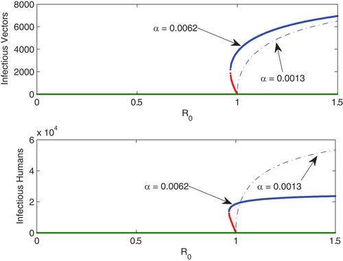
The result in (Figure 2) supports what we highlight in Theorem (4.3). For the set of parameters used in (Figure 2) we have $\mathcal{F}=0.0015,$ then when α = 0.0062 we have $\frac{{\mathcal{H}}_1}{k_2}+2d\alpha =7.8937\times {10}^{-4}$ and $\frac{\rho k_3{k}_4}{y_1^{\ast }}\sqrt{\frac{({\theta }_{1}d+{\theta }_2{k}_3)k_1{y}_1^{\ast }}{\beta \phi k_3(\gamma k_4-{\delta }_1\zeta \phi )x_1^{\ast }}}=3.4734\times {10}^{-5}.$ Therefore, $w_1{h}_{11}+w_2{h}_{21}>0$ (see Equation (31)(31) $\begin{array}{ll}{w}_1{h}_{11}+w_2{h}_{21}=& \frac{{\mathrm{\Delta }}_0{a}_{21}}{\rho k_3}[\frac{{\mathcal{H}}_1}{k_2}+2d\alpha \\ -\frac{\rho k_3{k}_4}{y_1^{\ast }}\sqrt{\frac{({\theta }_{1}d+{\theta }_2{k}_3)k_1{y}_1^{\ast }}{\beta \phi k_3(\gamma k_4-{\delta }_1\zeta \phi )x_1^{\ast }}}].\end{array}$(31) ) thus, ${\mathrm{\Delta }}_1<0$ and the bifurcation is backward. On the other hand, for α = 0.0013 we get $\frac{{\mathcal{H}}_1}{k_2}+2d\alpha =-2.7186\times {10}^{-5},$ causing $w_1{h}_{11}+w_2{h}_{21}$ to be negative. Therefore, the bifurcation is forward.

5. Uniform persistence

From an ecological point of view, persistence in a given community results when each species in the community is saved from extinction in the long run. In epidemic models, the analogy is: if a disease is proved to be persistent, then it is endemic, where every state variable (number in a disease compartment) is bounded away from zero. We establish that the disease is uniformly persistent in an environment when the secondary reproduction number is greater than one. To proceed, we first define a threshold η as a function of ɛ (to be used in Lemmas 5.1 and 5.2).

(36) $\begin{array}{ll}\eta (\epsilon )=\gamma k_1{k}_3{k}_4& [1-\frac{\zeta {\delta }_1\phi }{\gamma k_4}-\frac{{\varphi }^2\beta k(1-\epsilon )}{\gamma k_1{k}_3{k}_4}\\ \times ({\theta }_{1}d+{\theta }_2{k}_3)(y_1^{\ast }-\epsilon )(1/x_1^{\ast }-\epsilon )],\end{array}$(36)

where $k_1,k_3$ and k₄ are given by (4(4) $k_1=d+\mu ,k_2=\psi +\mu ,k_3=r+\alpha +\mu ,k_4=\phi +\gamma .$(4) ). Note that

(37) $\underset{\epsilon \to 0}{lim}\eta (\epsilon )=\gamma k_1{k}_3{k}_4(1-\frac{\zeta {\delta }_1\phi }{\gamma k_4}-{\mathcal{R}}_h^2).$(37)

Remark: $(1-\frac{\zeta {\delta }_1\phi }{\gamma k_4}-{\mathcal{R}}_h^2)<0$ for ${\mathcal{R}}_0>1.$

To see this, note that from (5(5) ${\mathcal{R}}_0={\mathcal{R}}_0(\zeta )=\frac{\zeta {\delta }_1\phi }{2\gamma k_4}+\sqrt{{\left(\frac{\zeta {\delta }_1\phi }{2\gamma k_4}\right)}^2+{\mathcal{R}}_h^2},$(5) ), $({\mathcal{R}}_0-\frac{\zeta {\delta }_1\phi }{2\gamma k_4}{)}^2=\frac{\zeta {\delta }_1\phi }{2\gamma k_4}+{\mathcal{R}}_h^2$ which is equivalent to

(38) ${\mathcal{R}}_0^2-{\mathcal{R}}_0\frac{\zeta {\delta }_1\phi }{\gamma k_4}={\mathcal{R}}_h^2.$(38)

Thus, when ${\mathcal{R}}_0>1$ we have ${\mathcal{R}}_0-\frac{\zeta {\delta }_1\phi }{2\gamma k_4}>1-\frac{\zeta {\delta }_1\phi }{2\gamma k_4}$ and since $\frac{\zeta {\delta }_1\phi }{2\gamma k_4}<1$ we have $1-\frac{\zeta {\delta }_1\phi }{2\gamma k_4}>0.$ This implies $({\mathcal{R}}_0-\frac{\zeta {\delta }_1\phi }{2\gamma k_4}{)}^2>(1-\frac{\zeta {\delta }_1\phi }{2\gamma k_4}{)}^2$ which is equivalent to ${\mathcal{R}}_0^2-\frac{{\mathcal{R}}_0\zeta {\delta }_1\phi }{\gamma k_4}>1-\frac{\zeta {\delta }_1\phi }{\gamma k_4}.$ Then using (38(38) ${\mathcal{R}}_0^2-{\mathcal{R}}_0\frac{\zeta {\delta }_1\phi }{\gamma k_4}={\mathcal{R}}_h^2.$(38) ), we have ${\mathcal{R}}_h^2>1-\frac{\zeta {\delta }_1\phi }{\gamma k_4}.$ Therefore, $1-\frac{\zeta {\delta }_1\phi }{\gamma k_4}-{\mathcal{R}}_h^2<0$ when ${\mathcal{R}}_0>1.$

In the following lemma and in Theorem (5.3), $int\mathrm{\Omega }$ represents the interior of Ω (the set is defined by (2(2) $\begin{array}{ll}\mathrm{\Omega }=& \{(X,Y)\in R_{+}^4\times R_{+}^3,\sum _{i=1}^4{x}_i\in [0,\frac{\rho }{\mu -\mathrm{\Lambda }}],\\ \sum _{i=1}^3{y}_i\in [0,\frac{{\delta }_0}{\gamma -{\delta }_1}]\}\\ =& \{X\in R_{+}^4,\sum _{i=1}^4{x}_i\in [0,\frac{\rho }{\mu -\mathrm{\Lambda }}]\}\times \\ \{Y\in R_{+}^3,\sum _{i=1}^3{y}_i\in [0,\frac{{\delta }_0}{\gamma -{\delta }_1}]\}\end{array}$(2) )).

Lemma 5.1.

Suppose $z_0\in int\mathrm{\Omega }$ such that the orbit $\mathrm{\Phi }(z_0,t)=z(t)$ approaches the disease-free equilibrium E₀ as $t\to \mathrm{\infty }$. Then, there is ɛ > 0 and a large t_o such that

$\begin{array}{l}\frac{\beta \varphi y_3{x}_1}{N}\ge \beta \varphi y_3(1-\epsilon )\end{array}$

and

$\begin{array}{l}\frac{\varphi {\theta }_1{x}_3{y}_1}{N}+\frac{\varphi {\theta }_2{x}_2{y}_1}{N}\ge \varphi ({\theta }_1{x}_3+{\theta }_2{x}_2)(y_1^{\ast }-\epsilon )(\frac{1}{x_1^{\ast }}-\epsilon )\\ \text{for}t\ge t_0.\end{array}$

Proof.

Since the orbit $\mathrm{\Phi }(z_0,t)=z(t)$ approaches E₀ as $t\to \mathrm{\infty }$, we have $\underset{t\to \mathrm{\infty }}{lim}\frac{1}{N(t)}=\frac{1}{x_1^{\ast }}$, $\underset{t\to \mathrm{\infty }}{lim}\frac{x_1(t)}{N(t)}=1$ and $\underset{t\to \mathrm{\infty }}{lim}{y}_1(t)=y_1^{\ast }.$ Moreover, given $\epsilon >0,$ there are large $t_1,$ t₂ and t₃ such that $\frac{1}{x_1^{\ast }}-\epsilon <\frac{1}{N}<\epsilon +\frac{1}{x_1^{\ast }}$ for all $t>t_3,$ $|\frac{x_1(t)}{N(t)}-1|<\epsilon$ for all $t\ge t_1$ and also $|y_1-y_1^{\ast }|<\epsilon$ for all $t\ge t_2$, which means $1-\epsilon <\frac{x_1(t)}{N(t)}$, $y_1>y_1^{\ast }-\epsilon$ for $t\ge t_0=max\{t_1,t_2,t_3\}$. These results lead to

$\begin{array}{l}\frac{\beta \varphi y_3{x}_1}{N}\ge \beta \varphi y_3(1-\epsilon )\end{array}$

and

$\begin{array}{l}\frac{\varphi {\theta }_1{x}_3{y}_1}{N}+\frac{\varphi {\theta }_2{x}_2{y}_1}{N}\ge \varphi ({\theta }_1{x}_3+{\theta }_2{x}_2)(y_1^{\ast }-\epsilon )(\frac{1}{x_1^{\ast }}-\epsilon )\\ \text{for}t\ge t_0.\end{array}$

Next, in preparation to establish the uniform persistence of system (1(1) $\begin{array}{ll}\frac{d{x}_1}{dt}& =\rho +\mathrm{\Lambda }N+\psi x_4-\frac{\beta \varphi y_3{x}_1}{N}-\mu x_1\\ \frac{d{x}_2}{dt}& =\frac{\beta \varphi y_3{x}_1}{N}-d{x}_2-\mu x_2\\ \frac{d{x}_3}{dt}& =d{x}_2-(r+\alpha +\mu )x_3\\ \frac{d{x}_4}{dt}& =r{x}_3-(\psi +\mu )x_4\\ \frac{d{y}_1}{dt}& ={\delta }_0+{\delta }_1(y_1+y_2)+{\delta }_1(1-\zeta )y_3-\frac{\varphi {\theta }_1{x}_3{y}_1}{N}\\ -\frac{\varphi {\theta }_2{x}_2{y}_1}{N}-\gamma y_1\\ \frac{d{y}_2}{dt}& =\frac{\varphi {\theta }_1{x}_3{y}_1}{N}+\frac{\varphi {\theta }_2{x}_2{y}_1}{N}+{\delta }_1\zeta y_3-\phi y_2-\gamma y_2\\ \frac{d{y}_3}{dt}& =\phi y_2-\gamma y_3,\end{array}$(1) ), we define a matrix

(39) $\mathcal{B}=\left(\begin{array}{ll}{\mathrm{\Theta }}_1& {\mathrm{\Theta }}_2\\ {\mathrm{\Theta }}_3& {\mathrm{\Theta }}_4\end{array}\right),$(39)

where

$\begin{array}{ll}{\mathrm{\Theta }}_1=& \left(\begin{array}{lll}-(d+{\mu }_1)& 0& 0\\ d& -(r+\alpha +{\mu }_1)& 0\\ 0& r& -(\psi +{\mu }_1)\end{array}\right),\\ {\mathrm{\Theta }}_2=& \left(\begin{array}{ll}0& \beta \varphi (1-\epsilon )\\ 0& 0\\ 0& 0\end{array}\right)\end{array}$

$\begin{array}{l}{\mathrm{\Theta }}_3=\left(\begin{array}{lll}\varphi {\theta }_2(y_1^{\ast }-\epsilon )(1/x_1^{\ast }-\epsilon )& \varphi {\theta }_1(y_1^{\ast }-\epsilon )(1/x_1^{\ast }-\epsilon )& 0\\ 0& 0& 0\end{array}\right),\end{array}$

$\begin{array}{l}{\mathrm{\Theta }}_4=\left(\begin{array}{ll}-(\phi +\gamma )& {\delta }_1\zeta \\ \phi & -\gamma \end{array}\right).\end{array}$

Lemma 5.2.

$\mathcal{B}$ has a positive eigenvalue when ${\mathcal{R}}_0>1.$

Proof.

We begin with the characteristic equation of $\mathcal{B}$ which is $f(h)=(h+k_2)(h^4+b_3{h}^3+b_2{h}^2+b_{1}h+b_0),$ where

(40) $\begin{array}{ll}{b}_3=& \gamma +k_1+k_3+k_4,b_2=k_3{k}_4+\gamma k_1-\phi {\delta }_1\zeta ,\\ b_1=& k_3{k}_4(\gamma +k_1)+\gamma k_1(k_3+k_4)-{\delta }_1\zeta (k_1+k_3)-{\varphi }^2{\theta }_2\beta (1-\epsilon )M,\\ b_0=& \gamma k_1{k}_3{k}_4[1-\frac{\zeta {\delta }_1\phi }{\gamma k_4}-\frac{{\varphi }^2\beta \phi (1-\epsilon )}{\gamma k_1{k}_3{k}_4}({\theta }_{1}d+{\theta }_2{k}_3)(y_1^{\ast }-\epsilon )(\frac{1}{x_1^{\ast }}-\epsilon )].\end{array}$(40)

Note that $b_0=\eta (\epsilon ),$ where $\eta (\epsilon )$ is given by (36(36) $\begin{array}{ll}\eta (\epsilon )=\gamma k_1{k}_3{k}_4& [1-\frac{\zeta {\delta }_1\phi }{\gamma k_4}-\frac{{\varphi }^2\beta k(1-\epsilon )}{\gamma k_1{k}_3{k}_4}\\ \times ({\theta }_{1}d+{\theta }_2{k}_3)(y_1^{\ast }-\epsilon )(1/x_1^{\ast }-\epsilon )],\end{array}$(36) ).

Thus, since $\underset{\epsilon \to 0}{lim}\eta (\epsilon )=\gamma k_1{k}_3{k}_4(1-\frac{\zeta {\delta }_1\phi }{\gamma k_4}-{\mathcal{R}}_h^2)<0$ and η is continuous as a function of ɛ, there is $0<\epsilon <\text{min}\{1,\frac{1}{x_1^{\ast }}\}$ such that $\eta (\epsilon )<0.$ Therefore, ${\mathcal{R}}_0>1$ ensures $b_0<0.$ Clearly the coefficient b₃ is positive. Also $b_2\ge (\frac{k_3}{\gamma }-1)\zeta {\delta }_1\phi +\gamma k_1$ is positive, which is possible if γ is reduced and α is increased. Regardless of the sign of b₁, there is exactly one change of sign in the coefficient sequence $\{b_0,b_1,b_2,b_3\}$. Therefore, by Descartes’s rule of sign (Anderson et al., 1998), $f(h)=0$ has one positive root when ${\mathcal{R}}_0>1$.

Theorem 5.3.

If ${\mathcal{R}}_0>1,$ the system given by (1(1) $\begin{array}{ll}\frac{d{x}_1}{dt}& =\rho +\mathrm{\Lambda }N+\psi x_4-\frac{\beta \varphi y_3{x}_1}{N}-\mu x_1\\ \frac{d{x}_2}{dt}& =\frac{\beta \varphi y_3{x}_1}{N}-d{x}_2-\mu x_2\\ \frac{d{x}_3}{dt}& =d{x}_2-(r+\alpha +\mu )x_3\\ \frac{d{x}_4}{dt}& =r{x}_3-(\psi +\mu )x_4\\ \frac{d{y}_1}{dt}& ={\delta }_0+{\delta }_1(y_1+y_2)+{\delta }_1(1-\zeta )y_3-\frac{\varphi {\theta }_1{x}_3{y}_1}{N}\\ -\frac{\varphi {\theta }_2{x}_2{y}_1}{N}-\gamma y_1\\ \frac{d{y}_2}{dt}& =\frac{\varphi {\theta }_1{x}_3{y}_1}{N}+\frac{\varphi {\theta }_2{x}_2{y}_1}{N}+{\delta }_1\zeta y_3-\phi y_2-\gamma y_2\\ \frac{d{y}_3}{dt}& =\phi y_2-\gamma y_3,\end{array}$(1) ) is uniformly persistent, that is, the boundary equilibrium E₀ is not the $\omega -$limit set of any orbit in intΩ, where Ω is given by (2(2) $\begin{array}{ll}\mathrm{\Omega }=& \{(X,Y)\in R_{+}^4\times R_{+}^3,\sum _{i=1}^4{x}_i\in [0,\frac{\rho }{\mu -\mathrm{\Lambda }}],\\ \sum _{i=1}^3{y}_i\in [0,\frac{{\delta }_0}{\gamma -{\delta }_1}]\}\\ =& \{X\in R_{+}^4,\sum _{i=1}^4{x}_i\in [0,\frac{\rho }{\mu -\mathrm{\Lambda }}]\}\times \\ \{Y\in R_{+}^3,\sum _{i=1}^3{y}_i\in [0,\frac{{\delta }_0}{\gamma -{\delta }_1}]\}\end{array}$(2) ).

Proof.

Recall that Ω is forward invariant under system (1(1) $\begin{array}{ll}\frac{d{x}_1}{dt}& =\rho +\mathrm{\Lambda }N+\psi x_4-\frac{\beta \varphi y_3{x}_1}{N}-\mu x_1\\ \frac{d{x}_2}{dt}& =\frac{\beta \varphi y_3{x}_1}{N}-d{x}_2-\mu x_2\\ \frac{d{x}_3}{dt}& =d{x}_2-(r+\alpha +\mu )x_3\\ \frac{d{x}_4}{dt}& =r{x}_3-(\psi +\mu )x_4\\ \frac{d{y}_1}{dt}& ={\delta }_0+{\delta }_1(y_1+y_2)+{\delta }_1(1-\zeta )y_3-\frac{\varphi {\theta }_1{x}_3{y}_1}{N}\\ -\frac{\varphi {\theta }_2{x}_2{y}_1}{N}-\gamma y_1\\ \frac{d{y}_2}{dt}& =\frac{\varphi {\theta }_1{x}_3{y}_1}{N}+\frac{\varphi {\theta }_2{x}_2{y}_1}{N}+{\delta }_1\zeta y_3-\phi y_2-\gamma y_2\\ \frac{d{y}_3}{dt}& =\phi y_2-\gamma y_3,\end{array}$(1) ) (Blayneh, 2017). Define a set $\mathcal{A}=\{(x_1,0,0,0,y_1,0,0):0<x_1\le \frac{\rho }{{\mu }_1-\lambda }\text{and}0<y_1\le \frac{{\delta }_0}{\gamma -{\delta }_1}\}$. Clearly $\bigcup _{z\in \mathcal{A}}\omega (z)=\{E_0\},$ where $E_0=(x_1^{\ast },0,0,0,y_1^{\ast },0,0)$ is the disease-free equilibrium of (1(1) $\begin{array}{ll}\frac{d{x}_1}{dt}& =\rho +\mathrm{\Lambda }N+\psi x_4-\frac{\beta \varphi y_3{x}_1}{N}-\mu x_1\\ \frac{d{x}_2}{dt}& =\frac{\beta \varphi y_3{x}_1}{N}-d{x}_2-\mu x_2\\ \frac{d{x}_3}{dt}& =d{x}_2-(r+\alpha +\mu )x_3\\ \frac{d{x}_4}{dt}& =r{x}_3-(\psi +\mu )x_4\\ \frac{d{y}_1}{dt}& ={\delta }_0+{\delta }_1(y_1+y_2)+{\delta }_1(1-\zeta )y_3-\frac{\varphi {\theta }_1{x}_3{y}_1}{N}\\ -\frac{\varphi {\theta }_2{x}_2{y}_1}{N}-\gamma y_1\\ \frac{d{y}_2}{dt}& =\frac{\varphi {\theta }_1{x}_3{y}_1}{N}+\frac{\varphi {\theta }_2{x}_2{y}_1}{N}+{\delta }_1\zeta y_3-\phi y_2-\gamma y_2\\ \frac{d{y}_3}{dt}& =\phi y_2-\gamma y_3,\end{array}$(1) ) and $\omega (z)$ is the omega limit set of a solution with initial $z\in \mathcal{A}$. Moreover, it should be noted that $\{E_0\}$ is isolated compact and invariant in Ω. To prove the uniform persistence of the disease, we need to prove that $\{E_0\}$ is a weak repeller for $int\mathrm{\Omega }$ (Thieme, 2004). The proof goes by contradiction. To begin with, suppose there is an initial point $z_0=(x_1^0,x_2^0,x_3^0,x_4^0,y_1^0,y_2^0,y_3^0)$ all positive components and $z_0\in int\mathrm{\Omega },$ such that the orbit $\mathrm{\Phi }(z_0,t)=z(t)$ approaches E₀ as $t\to \mathrm{\infty }$. By Lemma (5.1), there is ɛ > 0 and a large t₀, such that

$\begin{array}{l}\frac{\beta \varphi y_3{x}_1}{N}\ge \beta \varphi y_3(1-\epsilon )\end{array}$

and

$\begin{array}{l}\frac{\varphi {\theta }_1{x}_3{y}_1}{N}+\frac{\varphi {\theta }_2{x}_2{y}_1}{N}\ge \varphi ({\theta }_1{x}_3+{\theta }_2{x}_2)(y_1^{\ast }-\epsilon )(\frac{1}{x_1^{\ast }}-\epsilon )\\ \text{for}t\ge t_0.\end{array}$

Let $F(X,Y)=(f_1,f_2,f_3,f_4,f_5)$ be the vector field in Equation (1)(1) $\begin{array}{ll}\frac{d{x}_1}{dt}& =\rho +\mathrm{\Lambda }N+\psi x_4-\frac{\beta \varphi y_3{x}_1}{N}-\mu x_1\\ \frac{d{x}_2}{dt}& =\frac{\beta \varphi y_3{x}_1}{N}-d{x}_2-\mu x_2\\ \frac{d{x}_3}{dt}& =d{x}_2-(r+\alpha +\mu )x_3\\ \frac{d{x}_4}{dt}& =r{x}_3-(\psi +\mu )x_4\\ \frac{d{y}_1}{dt}& ={\delta }_0+{\delta }_1(y_1+y_2)+{\delta }_1(1-\zeta )y_3-\frac{\varphi {\theta }_1{x}_3{y}_1}{N}\\ -\frac{\varphi {\theta }_2{x}_2{y}_1}{N}-\gamma y_1\\ \frac{d{y}_2}{dt}& =\frac{\varphi {\theta }_1{x}_3{y}_1}{N}+\frac{\varphi {\theta }_2{x}_2{y}_1}{N}+{\delta }_1\zeta y_3-\phi y_2-\gamma y_2\\ \frac{d{y}_3}{dt}& =\phi y_2-\gamma y_3,\end{array}$(1) associated with the components $(x_2,x_3,x_4,y_2,y_3)$, in that order. Then $f_1\ge \beta \varphi (1-\epsilon )y_3-(d+{\mu }_1)x_2$ and $f_4\ge \varphi ({\theta }_1{x}_3+{\theta }_2{x}_2)(y_1^{\ast }-\epsilon )(\frac{1}{x_1^{\ast }}-\epsilon )+\zeta {\delta }_1{y}_3-(\phi +\gamma )y_2.$ The foregoing discussion leads to the following differential inequality.

(41) $\begin{array}{ll}\frac{d{x}_2}{dt}\ge & \beta \varphi (1-\epsilon )y_3-(d+{\mu }_1)x_2,\\ \frac{d{x}_3}{dt}\ge & d{x}_2-(r+\alpha +{\mu }_1)x_3\\ \frac{d{x}_4}{dt}\ge & r{x}_3-(\psi +{\mu }_1)x_4,\frac{d{y}_3}{dt}\ge \phi y_2-\gamma y_3\\ \frac{d{y}_2}{dt}\ge & \varphi ({\theta }_1{x}_3+{\theta }_2{x}_2)(y_1^{\ast }-\epsilon )(\frac{1}{x_1^{\ast }}-\epsilon )\\ +\zeta {\delta }_1{y}_3-(\phi +\gamma )y_2.\end{array}$(41)

Observe that the Jacobian of the new vector field, representing the right side of (41(41) $\begin{array}{ll}\frac{d{x}_2}{dt}\ge & \beta \varphi (1-\epsilon )y_3-(d+{\mu }_1)x_2,\\ \frac{d{x}_3}{dt}\ge & d{x}_2-(r+\alpha +{\mu }_1)x_3\\ \frac{d{x}_4}{dt}\ge & r{x}_3-(\psi +{\mu }_1)x_4,\frac{d{y}_3}{dt}\ge \phi y_2-\gamma y_3\\ \frac{d{y}_2}{dt}\ge & \varphi ({\theta }_1{x}_3+{\theta }_2{x}_2)(y_1^{\ast }-\epsilon )(\frac{1}{x_1^{\ast }}-\epsilon )\\ +\zeta {\delta }_1{y}_3-(\phi +\gamma )y_2.\end{array}$(41) ) at $(0,0,0,0,0)$ is $\mathcal{B}$, the matrix given by (39(39) $\mathcal{B}=\left(\begin{array}{ll}{\mathrm{\Theta }}_1& {\mathrm{\Theta }}_2\\ {\mathrm{\Theta }}_3& {\mathrm{\Theta }}_4\end{array}\right),$(39) ). Now consider the linear system $\frac{dz}{dt}=\mathcal{B}z.$ Note that $\mathcal{B}=(b_{ij}),i,j=1,\dots ,5$ has the following properties.

(i)

For every proper subset I of $N=\{1,2,3,4,5\},$ there is $i\in I$ and $j\in N\mathrm{\setminus }I$ such that $b_{ij}\ne 0.$ Thus, $\mathcal{B}$ is irreducible,

(ii)

$\mathcal{B}$ is quasi-positive that is, $b_{ij}\ge 0,i\ne j$ and $i,j\in \{1,\dots ,5\}$, then (i) and (ii) insure that $\mathcal{B}$ has a simple real eigenvalue which dominates the real parts of all eigenvalues of $\mathcal{B},$ that is, ${\lambda }_0>\mathrm{\Re }\vartheta ,\vartheta \in \sigma (\mathcal{B})(\text{note that }\mathrm{\Re }\vartheta \text{is the real part of}\vartheta )$ with a positive eigenvector v (Theorem A .45 in (Thieme, 2004)). Furthermore, this along with the result of Lemma (5.2) ensures that $\mathcal{B}$ has exactly one positive eigenvalue when ${\mathcal{R}}_0>1$. Consequently, ${\lambda }_0>0$. Now, pick an initial point $z(\tau )=(x_2(\tau ),x_3(\tau ),x_4(\tau ),y(\tau ),y_3(\tau ))$ on the manifold $rv:r>0,$ specifically $x_i(\tau )>r_0{v}_{i-1},i=2,3,4$, $y_2(\tau )>r_0{v}_4$ and $y_3(\tau )>r_0{v}_5$. Clearly, $\mathcal{B}v={\lambda }_{0}v>0$, then since the semiflow of $\frac{dz}{dt}=\mathcal{B}z$ is order preserving, the orbit $z(t,z(\tau ))$ goes to $+\mathrm{\infty }.$ Additionally, (41(41) $\begin{array}{ll}\frac{d{x}_2}{dt}\ge & \beta \varphi (1-\epsilon )y_3-(d+{\mu }_1)x_2,\\ \frac{d{x}_3}{dt}\ge & d{x}_2-(r+\alpha +{\mu }_1)x_3\\ \frac{d{x}_4}{dt}\ge & r{x}_3-(\psi +{\mu }_1)x_4,\frac{d{y}_3}{dt}\ge \phi y_2-\gamma y_3\\ \frac{d{y}_2}{dt}\ge & \varphi ({\theta }_1{x}_3+{\theta }_2{x}_2)(y_1^{\ast }-\epsilon )(\frac{1}{x_1^{\ast }}-\epsilon )\\ +\zeta {\delta }_1{y}_3-(\phi +\gamma )y_2.\end{array}$(41) ) implies that the solutions of $\frac{dz}{dt}=\mathcal{B}z$ are bounded from above by $(x_2(t),x_3(t),x_4(t),y_2(t),y_3(t))$ for all $t\ge \tau$ (Hall, 1969). This contradicts the fact that Ω is forward invariant under system (1(1) $\begin{array}{ll}\frac{d{x}_1}{dt}& =\rho +\mathrm{\Lambda }N+\psi x_4-\frac{\beta \varphi y_3{x}_1}{N}-\mu x_1\\ \frac{d{x}_2}{dt}& =\frac{\beta \varphi y_3{x}_1}{N}-d{x}_2-\mu x_2\\ \frac{d{x}_3}{dt}& =d{x}_2-(r+\alpha +\mu )x_3\\ \frac{d{x}_4}{dt}& =r{x}_3-(\psi +\mu )x_4\\ \frac{d{y}_1}{dt}& ={\delta }_0+{\delta }_1(y_1+y_2)+{\delta }_1(1-\zeta )y_3-\frac{\varphi {\theta }_1{x}_3{y}_1}{N}\\ -\frac{\varphi {\theta }_2{x}_2{y}_1}{N}-\gamma y_1\\ \frac{d{y}_2}{dt}& =\frac{\varphi {\theta }_1{x}_3{y}_1}{N}+\frac{\varphi {\theta }_2{x}_2{y}_1}{N}+{\delta }_1\zeta y_3-\phi y_2-\gamma y_2\\ \frac{d{y}_3}{dt}& =\phi y_2-\gamma y_3,\end{array}$(1) ). Thus, $\{E_0\}$ is a weak repeller for $int\mathrm{\Omega }$ (Thieme, 1993). This completes the proof.

6. Discussion and conclusion

One of the main challenges in disease control is failure to use the reduction of secondary reproduction number (${\mathcal{R}}_0$) below unity as means to predict disease elimination. This happens when a backward bifurcation exists. In this case, two endemic equilibrium points exist for ${\mathcal{R}}_0<1.$ We used a system of differential equations to study the dynamics of a vector-borne disease and conditions related to existence of a backward bifurcation. Our approaches implement analytical and simulation techniques. Bifurcation analysis of the model in Section (2) is presented in Section (3), where Theorem (4.3) reveals that when the disease-induced death rate in the host is reduced below a threshold value given by $\mathcal{F}$ there is no backward bifurcation, which means control efforts lead to disease elimination. 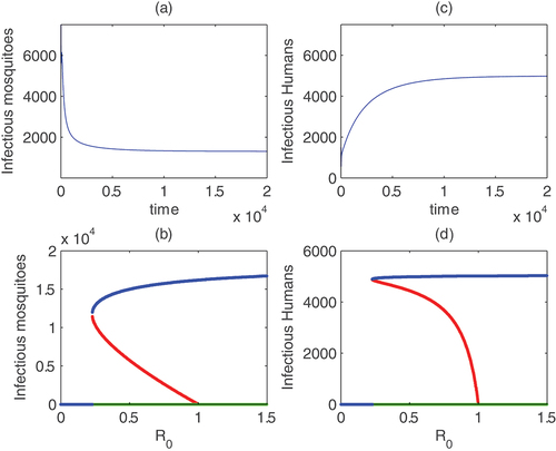Still, for some values of $\alpha >\mathcal{F},$ the bifurcation is forward however, but if α exceeds a critical value, then the disease becomes endemic. Increased mosquito level and disease transmission between mosquito and human play a role here. (Figure 2) offers numerical results regarding the backward bifurcation and parameters involved to this effect. Other challenges in a vertically transmitted vector-borne disease are related to transmissions of the disease from female mosquito to egg which is referred to as vertical transmission. Graphical results showing the effect of this transmission in raising the peak of epidemic are presented in (Figure 1). Numerical simulations are also presented where the infectious population from mosquitoes and humans approach endemic equilibrium levels in the long run even if ${\mathcal{R}}_0<1$ as given in (Figure 3).

Figure 3. Endemic asymptotic level of infectious mosquitoes and humans for ${\mathcal{R}}_0<1.$ ζ = 0.77 $\alpha =0.038,$ $\gamma =1/18,$ $\beta =0.87,{\theta }_1=0.0079,{\theta }_2=0.0072,$ $\mu =3.91\times {10}^{-5},\text{upLambda}=1.48\times {10}^{-5},\rho =200,{\delta }_0=1120,r=1/7,{\delta }_1=0.0397,d=1/6,\psi =0.00233,\varphi =2,\phi =1/8.$ for these set of parameters, ${\mathcal{R}}_0=0.3944<1,$ but mosquito and human populations equilibrate to endemic levels (see time plots (a) and (c) with initial value $(20,40,1500,40,2000,40,10000)$). The bifurcation diagrams of mosquitoes and humans as ${\mathcal{R}}_0$ changes given in windows (b) and (d) show backward bifurcations where two endemic equilibria exists for ${\mathcal{R}}_0<1$.

Moving forward, we like to clarify that baseline parameters which are widely used in the literature (see (Table 2)) are implemented in the numerical results of this article. We list some of them here. Estimation of parameters for mortality rate of mosquitoes such as Ades aegypti is based on the average life of mosquitoes which is from 14 to 17 days. The incubation period of dengue virus in a mosquito is from 7 to 14 days which is the base for estimating φ to be between $\frac{1}{14}$ and $\frac{1}{7}.$ Thus, we estimate φ by $\frac{1}{8}.$ Also, the recovery from dengue virus is about seven days, therefore, the recovery rate r is considered to be in $[0,\frac{1}{7}].$ In most developing countries, human (host) life expectancy (in years) is in the range from 45 to 70. Accordingly, human mortality rate is estimated to be in the interval $[\frac{1}{70(365)},\frac{1}{45(365)}].$ Disease transmission rate from exposed hosts, θ₂ is estimated to be $0.0063,$ and it is less than θ₁ which is estimated to be $0.0083,$ θ₁ is transmission from infectious hosts to mosquitoes.

Table 2. Parameter estimation for dengue fever. Rate is per day

Par.	Range	Ref.	Par.	Range	Ref.
γ	$[1/17,1/10]$	(Centers for Disease Control and Prevention: Malaria)	δ0	$[700,10,000]$	estimate
µ	$[\frac{1}{70(356)},\frac{1}{45(356)}]$	(WHO)	θ1	$[0,1)$	estimate
ϕ	$\ge 1$	variable	α	$(0,0.1)$	Chitnis et al. (2013), (WHO)
φ	$[1/14,1/7]$	Chan et al. (2012)	ψ	$[0,1)$	estimate
r	$[0,1/7]$	Adams and Boots (2010)	β	$(0,1)$	estimate
ζ	$[0,1)$	estimate	δ1	$[0,\gamma )$	estimate
d	$[1/14,1/3]$	(Centers for Disease Control and Prevention)	ρ	$\ge 1$	variable
θ2	$[0,{\theta }_1)$	estimate
Λ	$(0,\mu )$	estimate

(Figure 1) is interpreted as follows: Vertical transmission of the disease in the mosquito population increases epidemic level. Keeping other parameters fixed, we increased the vertical transmission rate $\zeta .$ We selected three different values, namely $0.0046,$ 0.3046 and $0.5046,$ then observed that an increase of this rate by $30\mathrm{\%}$ causes the epidemic level to increase. The pick epidemic level is higher for a $50\mathrm{\%}$ increase in vertical transmission rate. These results are represented graphically in (Figure 1). It should be clear that in each case the secondary reproduction number, ${\mathcal{R}}_0,$ is less than unity: here are the corresponding values: ${\mathcal{R}}_0=0.0673$ ($\zeta =0.0046),$ ${\mathcal{R}}_0=0.1662$ ($\zeta =0.3046)$ and ${\mathcal{R}}_0=0.2492$ ($\zeta =0.5046).$ If disease prevention efforts focus on adult as well as larva control, then the effect of this transmission on raising the epidemic level could be diminished.

Simulation results given in (Figure 2) illustrate some of the conclusions drawn from Theorem (4.3). The data and estimation of key parameters are based on dengue virus and supporting references are provided in (Table 2). In this theorem, a backward bifurcation is possible when ${\mathrm{\Delta }}_1<0,$ which is the coefficient of ϵ in the Lyapunov–Smith expansion given by Equation (25)(25) $\begin{array}{ll}x& =ϵV+{ϵ}^{2}U+\mathcal{O}({ϵ}^3)\\ \mathrm{\Delta }& ={\mathrm{\Delta }}_0+ϵ{\mathrm{\Delta }}_1+\mathcal{O}({ϵ}^2),\text{where}\end{array}$(25) . Additionally, the sign of $w_1{h}_{11}+w_2{h}_{12}$ and Δ₁ are opposite (see (30(30) ${\mathrm{\Delta }}_1=-\frac{(w_1{h}_{11}+w_2{h}_{21})}{a_{12}{w}_1{v}_2+a_{21}{w}_2{v}_1}.$(30) )). Furthermore, the theorem establishes that reduction of the disease-induced death rate, $\alpha ,$ below a threshold denoted by $\mathcal{F}$ will eliminate backward bifurcation. Backward bifurcation is a phenomena where endemic equilibrium points exist despite managing to reduce the secondary reproduction number below unity. The main bifurcation result in connection with model parameters states that the sign of the right term in Equation (31)(31) $\begin{array}{ll}{w}_1{h}_{11}+w_2{h}_{21}=& \frac{{\mathrm{\Delta }}_0{a}_{21}}{\rho k_3}[\frac{{\mathcal{H}}_1}{k_2}+2d\alpha \\ -\frac{\rho k_3{k}_4}{y_1^{\ast }}\sqrt{\frac{({\theta }_{1}d+{\theta }_2{k}_3)k_1{y}_1^{\ast }}{\beta \phi k_3(\gamma k_4-{\delta }_1\zeta \phi )x_1^{\ast }}}].\end{array}$(31) will determine the direction of bifurcation. We list what the connection between this theorem and the numerical results in (Figure 2) where estimation of parameters is done based on dengue virus . For the set of parameters used in (Figure 2), we have $\mathcal{F}=0.0015.$ Clearly, for $\alpha =0.0013<0.0015,$ the bifurcation is forward. However, when $\alpha =0.0062>\mathcal{F},$ the bifurcation is backward, as the sign of ${\mathrm{\Delta }}_1<0.$ For this value of $\alpha ,$ $\frac{{\mathcal{H}}_1}{k_2}+2d\alpha =7.8937\times {10}^{-4}$ and $\frac{\rho k_3{k}_4}{y_1^{\ast }}\sqrt{\frac{({\theta }_{1}d+{\theta }_2{k}_3)k_1{y}_1^{\ast }}{\beta \phi k_3(\gamma k_4-{\delta }_1\zeta \phi )x_1^{\ast }}}=3.4734\times {10}^{-5}.$ Some numerical results could support the fact that having $\alpha >\mathcal{F}$ may not alone change the bifurcation result. For example, in addition to value of α used in (Figure 2), at $\alpha =0.0016,$ $\frac{{\mathcal{H}}_1}{k_2}+2d\alpha -\frac{\rho k_3{k}_4}{y_1^{\ast }}\sqrt{\frac{({\theta }_{1}d+{\theta }_2{k}_3)k_1{y}_1^{\ast }}{\beta \phi k_3(\gamma k_4-{\delta }_1\zeta \phi )x_1^{\ast }}}=2.2807\text{break}\times {10}^{-5}-3.3980\times {10}^{-5}=-1.1172\times {10}^{-6}$. The bifurcation analysis used here help point the role played by the fatality of the disease as measured by the parameter for disease-induced death rate.

As it is explained early, what is given in (Figure 3) is that when there is backward bifurcation, solutions with some initial value equilbrate to a positive value even if ${\mathcal{R}}_0<1.$ The graphs of the infectious populations are plotted. From this one can conclude that the other components, such as exposed also approach an endemic equilibrium levels. Although in Section (5), persistence of the disease is established for ${\mathcal{R}}_0>1,$ the result we see in (Figure 3) suggested possibility of persistence of the disease when conditions for backward bifurcation are met. It should be noted that for the set of parameter values used in (Figure 3), ${\mathcal{R}}_0=0.3944$ which is less than one.

Based on our model, without vector-host transmission cycle, vertical transmission alone, cannot cause the disease to be endemic or create a backward bifurcation phenomena. However, vertical transmission in the vector could increase the prevalence and epidemic level of the disease in the vector and host populations. Therefore, efforts to mitigate the effects of vertical transmissions which primarily should focus on mosquito control as well as improved measures against disease transmission, such as strong personal protection. Furthermore, disease-induced death rate, if kept low may not cause endemic equilibrium, this means as long as the secondary reproduction number, ${\mathcal{R}}_0,$ is kept below one, the disease could not establish in a given community. If mosquito level and mosquito-human disease transmission cycles are increased and the disease-induced death rate in hosts passes a critical level, then the disease could be endemic even when ${\mathcal{R}}_0,$ is reduced below one. We conjecture that there could be a critical value of this threshold, below which disease elimination is possible. When the secondary reproduction number is increased beyond one, the disease is uniformly persistent, each disease compartment is bounded away from zero.

Disclosure statement

No potential conflict of interest was reported by the author(s).

References

- Adams, B., & Boots, M. (2010). How important is vertical transmission in mosquitoes for the persistence of dengue? Insights from a mathematical model. Epidemics, 2(1), 1–10. https://doi.org/10.1016/j.epidem.2010.01.001
- Allen, L. (2007). An introduction to mathematical biology. Pearson Prentice Hall.
- Anderson, B., Jackson, J., & Sitharam, M. (1998). Descarte’s rule of signs revisited. The American Mathematical Monthly, 105(5), 447–451. https://doi.org/10.1080/00029890.1998.12004907
- Blayneh, K. W. (2017). Vertically transmitted vector-borne diseases and the effects of extreme temperature. International Journal of Apllied Mathematics, 30(2), 177–209. https://doi.org/10.12732/ijam.v30i2.8
- Blayneh, K., Cao, Y., & Kwon, H.-D. (2009). Optimal control of vector-borne diseases: Treatment and prevention. Discrete and Continuous Dynamical Systems Series B, 11(3), 587–611. https://doi.org/10.3934/dcdsb.2009.11.587
- Blayneh, K. W., Gumel, A. B., Lenhart, S., & Clayton, T. (2010). Backward bifurcation and optimal control in transmission dynamics of West Nile virus. Bulletin of Mathematical Biology, 72(4), 1006–1028. https://doi.org/10.1007/s11538-009-9480-0
- Centers for Disease Control and Prevention. http://www.cdc.gov/dengue
- Centers for Disease Control and Prevention: Malaria. http://www.cdc.gov/Malaria/faq.htm2
- Chan, M., Johansson, M. A., & Vasilakis, N. (2012). The incubation periods of dengue viruses. PLoS ONE, 7(11), e50972. https://doi.org/10.1371/journal.pone.0050972
- Chitnis, N., Cushing, J. M., & Hyman, J. M. (2006). Bifurcation analysis of a mathematical model for malaria transmission. SIAM Journal on Applied Mathematics, 67(1), 24–45. https://doi.org/10.1137/050638941
- Chitnis, N., Hyman, J. M., & Manore, C. A. (2013). Modelling vertical transmission in vector-borne diseases with application to Rift Valley fever. Journal of Biological Dynamics, 7(1), 11–40. https://doi.org/10.1080/17513758.2012.733427
- Cruz-Pacheco, G., Esteva, L., & Vargas, C. (2009). Seasonality and outbreaks in West Nile varus infection. Bulletin of Mathematical Biology, 71(6), 1378–1393. https://doi.org/10.1007/s11538-009-9406-x
- Cushing, J. M. (1998). An introduction to structured population dynamics. SIAM.
- Dushoff, J., Wenzhang, H., & Castillo-Chavez, C. (1998). Backwards bifurcations and catastrophe in simple models of fatal diseases. Journal of Mathematical Biology, 36(3), 227–248. https://doi.org/10.1007/s002850050099
- Feng, Z., & Velasco-Hernández, J. X. (1997). Competitive exclusion in a vector-host model for the dengue fever. Journal of Mathematical Biology, 35(5), 523–544. https://doi.org/10.1007/s002850050064
- Francisco, P. M. (2007). Factors affecting the emergence and prevalence of vector borne infections and the role of vertical transmission. Journal of Vector Borne Diseases, 44, 157–163.
- Gaff, H. D., Hartley, D. M., & Leahy, N. P. (2007). An epidemiological model of Rift Valley fever. Electronic Journal of Differential Equations, 2007(115), 1–12.
- Gordillo, L. F. (2013). Reducing mosquito-borne disease outbreak size: The relative importance of contact and tranmissibility in a network model. Applied Mathematical Modeling, 37(18–19), 8610–8616. https://doi.org/10.1016/j.apm.2013.03.056
- Gourley, S. A., Röst, G., & Thieme, H. R. (2014). Uniform persistence in a model for bluetongue dynamics. SIAM Journal on Mathematical Analysis, 46(2), 1160–1184. https://doi.org/10.1137/120878197
- Hall, J. K. (1969). Ordinary differential equations. Wiley-Interscience.
- Hubálek, Z., & Halouzka, J. (1999). West Nile fever. A reemerging mosquito-borne viral disease in Europe. Emerging Infectious Diseases, 5(5), 643–650. https://doi.org/10.3201/eid0505.990505
- Joseph, W., So, H., & Freedman, H. I. (1986). Persistence and global stability in a predator-prey model consisting of three prey genotypes with fertility differences. Bulletin of Mathematical Biology, 48(5), 469–484. https://doi.org/10.1016/S0092-8240(86)90002-9
- Pu, L., Lin, Z., & Lou, Y. (2023). A West Nile virus nonlocal model with free boundaries and seasonal succession. Journal of Mathematical Biology, 86(2), 25. https://doi.org/10.1007/s00285-022-01860-x
- Rabinowitz, P. H. (1971). Some global results for nolinear eigenvalue problems. Journal of Functional Analysis, 7(3), 487–513. https://doi.org/10.1016/0022-1236(71)90030-9
- Robelo, C., Margheri, A., & Bacaër, N. (2014). Persistence in some periodic epidemic models with infection age or constant periods of infection. Discrete and Continuous Dynamical Systems-Series B(DCDS-B), 19(4), 1155–1170. https://doi.org/10.3934/dcdsb.2014.19.1155
- Salako, R. B. (2023). The impact of population size and movement on the persistence of a two-strain infectious disease. Journal of Mathematical Biology, 86(1), 5. https://doi.org/10.007/s00285-022-01842-z
- Stakgold, I. (1979). Green’s functions and boundary value problems. Wiley-Interscience.
- Thieme, H. R. (1993). Persistence under relaxed point-dissipativity (with applications to an epidemic model). SIAM Journal on Mathematical Analysis, 24(2), 407–435. https://doi.org/10.1137/0524026
- Thieme, H. R. (2001). Disease extinction and disease persistence in age structured epidemic models, H.R. Thieme, nonlinear analysis, theory. Methods & Applications, 47(9), 6181–6194. https://doi.org/10.1016/S0362-546X(01)00677-0
- Thieme, H. R. (2004). Mathematics in population biology, Princeton series in theoretical and computational Biology. Princeton.
- van den Driessche, P., & Watmough, J. (2002). Reproduction numbers and sub-threshold endemic equibria for compartmental models of disease transmission. Mathematical Biosciences, 180(1–2), 29–48. https://doi.org/10.1016/S0025-5564(02)00108-6
- van den Driessche, P., & Yakubu, A.-A. (2019). Disease extinction versus persistence in discrete-time epidemic models. Bulletin of Mathematical Biology, 81(11), 4412–4446. https://doi.org/10.1007/s11538-018-0426-2
- Wang, X., Chen, Y., & Martcheva, M. (2020). Asymptotic analysis of a vector-borne disease model with the age of infection. Journal of Biological Dynamics, 14(1), 332–367. https://doi.org/10.1080/17513758.2020.1745912
- WHO. https://who.int/news-room/fact-sheets/detail/dengue-and-sever-dengue.
- Zheng, B. (2022). Impact of releasing period and magnitude on mosquito population in a sterile release model with delay. Journal of Mathematical Biology, 85(2), 18. https://doi.org/10.1007/s00285-022-01785-5
- Zhu, Z., Hui, Y., & Hu, L. (2023). The impact of predators of mosquito larvae on wolbachia spreading dynamics. Journal of Biological Dynamics, 17(1), 1. https://doi.org/10.1080/17513758.2023.2249024