Sensitivity analysis for active electromagnetic field manipulation in free space

ABSTRACT

This paper presents a detailed sensitivity analysis of the active manipulation scheme for electromagnetic (EM) fields in free space. The active EM fields control strategy is designed to construct surface current sources (electric and/or magnetic) that can manipulate the EM fields in prescribed exterior regions. The active EM field control is formulated as an inverse source problem. We follow the numerical strategies in our previous works, which employ the Debye potential representation and integral equation representation in the forward modelling. We consider two regularization approaches to the inverse problem to approximate a current source, namely the truncated singular value decomposition (TSVD) and the Tikhonov regularization with the Morozov discrepancy principle. Moreover, we discuss the sensitivity of the active scheme (concerning power budget, control accuracy, and quality factor) as a function of the frequency, the distance between the control region and the source, the mutual distance between the control regions, and the size of the control region. The numerical simulations demonstrate some challenges and limitations of the active EM field control scheme.

KEYWORDS:

• Active EM field control
• Maxwell's equations
• Debye potentials
• integral equations
• inverse source problem

AMS:

• 45A05
• 65E05
• 78A46
• 78M15
• 45Q05

1. Introduction

Active manipulation of electromagnetic (EM) fields is emerging in modern electromagnetics. In recent years, the study of active field control techniques has attracted huge attention and research efforts. The current literature has significantly addressed the idea of the active control of the EM fields in broad applications. These applications include, but are not limited to, scattering cancellation or reduction [1–8], metamaterial or metasurface design [9–14], field synthesis [15–22]. Active field control techniques are becoming increasingly ubiquitous to enhance EM wave-based systems.

Regarding the scattering cancellation or reduction (also known as cloaking) applications, Chen et al. [1] demonstrated active scattering-cancellation cloaks in both 1-D and 3-D scenarios. The authors explored the potential of active scattering-cancellation cloaks to realize broadband invisibility based on anomalous permittivity dispersion. Theoretically, the proposed active cloak scheme can overcome the Bode–Fano bandwidth limit and operate in a much broader bandwidth than passive scattering-cancellation cloaks. Onofrei [8] investigated the active cloaking in the quasi-static regime, where the field is modelled by the Laplace operator. In this work, the author proposed a systematic integral equation method to generate suitable quasi-static fields for cloaking, illusions and energy focussing (with given accuracy) in multiple regions of interest. In [2], the authors proposed an active cloaking mechanism that makes use of the equivalence principle. In this approach, the cylinder is replaced by an array of electric or magnetic current sources placed around the cylinder's periphery. Then the equivalent currents radiate in free space. Another circular array of current sources is placed concentrically to the original cylindrical object. Excitations of these external sources are taken such that the array and the object cancel its overall scattering for an incoming wave. Similarly, Selvanayagam et al. [6] investigated the active EM cloak using the equivalence principle. Additional electric and magnetic currents are introduced to cancel out the scattered fields from the object. Electric and magnetic dipoles can respectively replace the electric and magnetic currents. It has been proven that this approach can realize both exterior and interior cloaking. Moreover, scattering reduction is widespread in the radar system. The authors in [7] proposed a general real-time radar cross-section (RCS) reduction scheme to reduce the transient scattered signal from an object. They used a sensor on the object to measure the incident signal and applied a microstrip antenna to produce the cancelling signal. The authors assume that the direction of an incident signal at the receiver is known. The radiation from the defending antenna can be adjusted in real-time to cancel the scattering from the object. Thus the total field at the distant receiver is negligible so that the object becomes invisible to a radar working in a given known frequency band. The active field control techniques are also prevalent in metamaterial or metasurface design. In [9], Brown et al. explored the possibility of metasurface design by making use of the electromagnetic inverse source framework. The electric and magnetic surface susceptibility profiles are computed such that the transmitted field exhibits the desired field specifications. The results show that the metasurface can focus the beam from plane wave, change the direction and radiation pattern, etc. Huang et al. [13] reported a reconfigurable metasurface for multifunctional control of EM waves. The proposed metasurface can generate beam-splitting performance to reduce backward scattering waves. Research into new active field manipulation methods can play an important role in field synthesis applications. Classically, the problem of field synthesis seeks to construct the necessary currents on a source such that the source can produce a given field pattern [23]. Lopéz et al. [20] proposed a source reconstruction method (SRM) to establish the equivalent current distribution that radiates the same field as the actual current induced in the antenna under test (AUT). The target application is antenna diagnostics. The knowledge of the equivalent currents allows the determination of the antenna radiating elements and the prediction of the AUT-radiated fields outside the equivalent currents domain. Ayestarán et al. [15] introduced an array synthesis technique that can focus the near-field (NF) on one or more spots and simultaneously satisfy the far-field (FF) specifications. This array synthesis technique can be applied to wireless power transfer. Wireless links between the antenna array and devices are established more efficiently since power radiated at undesired positions or directions can be suppressed.

The majority of the efforts in the literature mentioned above have been focussed on developing new approaches for active EM field control. One of the standard control strategies is based on the equivalence principle. Another category makes use of the transformation acoustics or transformation optics techniques. These works give insight into the performance of the proposed approaches under certain situations, such as narrow frequency bands, limited control geometry, and fixed size of the sources. However, the performances of the control strategies are unrevealed when the problem parameters are changed. In addition, the evaluation of the control performance in previous literature is limited, i.e. only based on the control accuracy. Therefore, a detailed sensitivity study for the problem of controlling three-dimensional EM fields in prescribed exterior regions in free space is presented. To our best knowledge, this is the first work to investigate the sensitivity of the active scheme concerning the problem parameters. Following the similar procedure in our previous publications [24–29], the active manipulation of the EM fields is formulated as an inverse source-type problem, which addresses the source reconstruction from the knowledge of the field outside the source region [30–32]. We discuss the sensitivity of the active scheme (concerning power budget, control accuracy, and quality factor) as a function of the frequency, the distance between the control region and the source, the mutual distance between the control regions, and the size of the control region. In our previous work [33], we demonstrated a feasibility study of actively manipulating EM fields in free space. The paper mainly used integral equation method in the forward modelling and the truncated singular value decomposition (TSVD) method to solve matrix inversion. Besides, the paper is limited to the one-region control. In this work, we introduce two approaches for forward modelling and two approaches for inversion, respectively. We also extend our framework into multiple-region control, especially in contrast control. The contrast EM fields will pose control challenges as the control regions cannot be placed very close to each other.

The rest of this paper is organized as follows. In Section 2, we formally describe the problem and provide relevant theoretical results obtained in [29]. We apply two methods in the forward modelling, including the Debye potential approach and the integral equation method. Two approaches are used to solve the inverse problem, including the truncated singular value decomposition (TSVD) and the Tikhonov regularization with the Morozov discrepancy principle. Section 3 shows the numerical results of the benchmark examples. Section 4 presents the EM field control sensitivity analysis in free space. Finally, we conclude the paper with some remarks in Section 5.

2. Theory

2.1. Problem formulation

This section presents a general description of the active manipulation scheme for EM fields. The unified functional and numerical framework have already been discussed in [26–29]. Though some of those works addressed the problem of controlling the Helmholtz fields, the approach could be extended to solve the EM problems governed by Maxwell's equations. We shall briefly recall several essential theoretical results and describe some geometric configurations of interest.

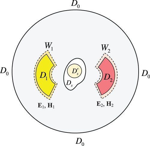
This paper explores the active EM fields manipulation scheme in free space. The problem geometry is sketched in Figure 1. Here we only consider a single source $D_s$, two control regions $D_1$ and $D_2$ for illustrative purposes. Note that the theoretical analysis in [26,28,29,34] indicates that an arbitrary number of source regions and exterior control regions can be considered in the active control scheme. The control regions $D_1$ and $D_2$ are mutually disjoint smooth domains, i.e. $D_1\cap D_2=\mathrm{\varnothing }$. We also make the assumption that the control regions are well-separated from the source region, i.e. $(D_1\cup D_2)\cap D_s=\mathrm{\varnothing }$. Considering the EM wave in a homogeneous isotropic source free medium in ${\mathbb{R}}^3$, the wave propagation is governed by Maxwell's equations, (1) $\mathrm{\nabla }\times \mathbf{E}=i\omega \mu \mathbf{H};\mathrm{\nabla }\times \mathbf{H}=-i\omega ϵ\mathbf{E}.$(1) where ε and μ is the electric permittivity and magnetic permeability of the homogeneous and isotropic medium, yielding ${ϵ}_0$ and ${\mu }_0$ in free space. The time-harmonic factor $e^{-i\omega t}$ is assumed but suppressed in the following demonstration.

Figure 1. Sketch of the problem geometry showing the control regions $D_1$, $D_2$ and the source region $D_s$ in free space.

The inverse source problem addresses the source reconstruction from the knowledge of the field outside the source region. It is often desirable to find the necessary sources that produce the given EM fields in the prescribed exterior regions. Mathematically, the problem is to find the boundary input on the source, either surface electric current $\mathbf{J}\in C^{\mathrm{\infty }}\left(\mathrm{\partial }{D}_s\right)$ or magnetic current $\mathbf{M}\in C^{\mathrm{\infty }}\left(\mathrm{\partial }{D}_s\right)$ such that the solutions $(\mathbf{E},\mathbf{H})$ of (2) $\{\begin{array}{l}\mathrm{\nabla }\times \mathbf{E}=i\omega \mu \mathbf{H},\mathrm{\nabla }\times \mathbf{H}=-i\omega ϵ\mathbf{H}\text{in}{\mathbb{R}}^3\setminus D_s,\\ \mathbf{E}\times \mathbf{n}=\mathbf{M},(\text{or}\mathbf{n}\times \mathbf{H}=\mathbf{J})\text{on}\mathrm{\partial }{D}_s,\\ (\mathbf{E},\mathbf{H})\text{satisfy the Silver-Muller radiation condition at infinity,}\end{array}$(2) satisfy the control constraints (3) $\{\begin{array}{ll}\Vert \mathbf{E}-{\mathbf{E}}_j{\Vert }_{C\left(D_j\right)}\le \delta & \mathrm{f}\mathrm{o}\mathrm{r}j=\overline{1,2},\\ \Vert \mathbf{H}-{\mathbf{H}}_j{\Vert }_{C\left(D_j\right)}\le \delta & \mathrm{f}\mathrm{o}\mathrm{r}j=\overline{1,2},\end{array}$(3) where δ is the desired control accuracy threshold. In (2(2) $\{\begin{array}{l}\mathrm{\nabla }\times \mathbf{E}=i\omega \mu \mathbf{H},\mathrm{\nabla }\times \mathbf{H}=-i\omega ϵ\mathbf{H}\text{in}{\mathbb{R}}^3\setminus D_s,\\ \mathbf{E}\times \mathbf{n}=\mathbf{M},(\text{or}\mathbf{n}\times \mathbf{H}=\mathbf{J})\text{on}\mathrm{\partial }{D}_s,\\ (\mathbf{E},\mathbf{H})\text{satisfy the Silver-Muller radiation condition at infinity,}\end{array}$(2) ), $\mathbf{n}$ denotes the unit exterior normal vector to $D_s$. The Silver-Muller radiation condition in (2(2) $\{\begin{array}{l}\mathrm{\nabla }\times \mathbf{E}=i\omega \mu \mathbf{H},\mathrm{\nabla }\times \mathbf{H}=-i\omega ϵ\mathbf{H}\text{in}{\mathbb{R}}^3\setminus D_s,\\ \mathbf{E}\times \mathbf{n}=\mathbf{M},(\text{or}\mathbf{n}\times \mathbf{H}=\mathbf{J})\text{on}\mathrm{\partial }{D}_s,\\ (\mathbf{E},\mathbf{H})\text{satisfy the Silver-Muller radiation condition at infinity,}\end{array}$(2) ) at infinity is defined as (4) $\{\begin{array}{l}\mathbf{E}\left(\mathbf{x}\right)\times \hat{\mathbf{x}}+\frac{1}{Y}\mathbf{H}\left(\mathbf{x}\right)=O\left(1/|\mathbf{x}{|}^2\right),\\ \mathbf{H}\left(\mathbf{x}\right)\times \hat{\mathbf{x}}-Y\mathbf{E}\left(\mathbf{x}\right)=O\left(1/|\mathbf{x}{|}^2\right),\end{array}$(4) as $|\mathbf{x}|\to \mathrm{\infty }$ uniformly with respect to points $\hat{\mathbf{x}}$ in the unit sphere S. $Y=\sqrt{\frac{ϵ}{\mu }}$ is the admittance in non-conductive media. The radiation conditions can be simply rewritten for all the equivalent forms of the Maxwell system and giving a smooth enough boundary data, they guarantee the uniqueness of solutions for Maxwell exterior problems [35].

2.2. Debye potential representation

We present two approaches for the numerical computation of EM fields from the surface currents in the following subsections. The first one is the Debye potential representation that expresses the vector EM fields in terms of two scalar Debye potentials [36–38]. This approach gives rise to a pair of scalar inverse source problems involving the Helmholtz equation as discussed in [26–29]. Firstly, we rewrite Maxwell's equations in (1(1) $\mathrm{\nabla }\times \mathbf{E}=i\omega \mu \mathbf{H};\mathrm{\nabla }\times \mathbf{H}=-i\omega ϵ\mathbf{E}.$(1) ) as (5) $\mathrm{\nabla }\times \tilde{\mathbf{E}}=ik\tilde{\mathbf{H}},\mathrm{\nabla }\times \tilde{\mathbf{H}}=-ik\tilde{\mathbf{E}},$(5) by introducing the transformation pair $\tilde{\mathbf{E}}=\sqrt{ϵ}\mathbf{E},\tilde{\mathbf{H}}=\sqrt{\mu }\mathbf{H}$. The k in (5(5) $\mathrm{\nabla }\times \tilde{\mathbf{E}}=ik\tilde{\mathbf{H}},\mathrm{\nabla }\times \tilde{\mathbf{H}}=-ik\tilde{\mathbf{E}},$(5) ) is the wavenumber and $k=\omega \sqrt{\mu ϵ}$. Then, we define two vector fields $\mathbf{A}$ and $\mathbf{B}$, where $\mathbf{A}=\sqrt{-iϵ\omega }\mathbf{E},\mathbf{B}=\sqrt{i\omega \mu }\mathbf{H}$, equivalently satisfy (6) $\mathrm{\nabla }\times \mathbf{A}=k\mathbf{B},\mathrm{\nabla }\times \mathbf{B}=k\mathbf{A}.$(6) Equation (6(6) $\mathrm{\nabla }\times \mathbf{A}=k\mathbf{B},\mathrm{\nabla }\times \mathbf{B}=k\mathbf{A}.$(6) ) is called the Wilcox form of the Maxwell's equations [39]. It has been proved in [39] that there exists unique $u_j,v_j$ (with zero average over the unit ball) solutions of Helmholtz equation in $D_j$ for each $j=\overline{1,2}$ given by the following weakly singular integral operators, (7) $\{\begin{array}{l}{u}_j\left(r\hat{\mathbf{r}}\right)=-{\displaystyle \frac{r}{2\pi }{\int }_{B_1}[\log (\sin \frac{\gamma }{2}\left)\right]\hat{\mathbf{r}}\cdot {\mathbf{A}}_j\left(r\widehat{{\mathbf{r}}^{\mathrm{\prime }}}\right)\mathrm{d}S,}\\ v_j\left(r\hat{\mathbf{r}}\right)=-{\displaystyle \frac{r}{2\pi }{\int }_{B_1}[\log (\sin \frac{\gamma }{2}\left)\right]\hat{\mathbf{r}}\cdot {\mathbf{B}}_j\left(r\widehat{{\mathbf{r}}^{\mathrm{\prime }}}\right)\mathrm{d}S,}\end{array}$(7) where $B_x$ denotes the ball centred at the origin and the radius is x, i.e. $B_1$ in (7(7) $\{\begin{array}{l}{u}_j\left(r\hat{\mathbf{r}}\right)=-{\displaystyle \frac{r}{2\pi }{\int }_{B_1}[\log (\sin \frac{\gamma }{2}\left)\right]\hat{\mathbf{r}}\cdot {\mathbf{A}}_j\left(r\widehat{{\mathbf{r}}^{\mathrm{\prime }}}\right)\mathrm{d}S,}\\ v_j\left(r\hat{\mathbf{r}}\right)=-{\displaystyle \frac{r}{2\pi }{\int }_{B_1}[\log (\sin \frac{\gamma }{2}\left)\right]\hat{\mathbf{r}}\cdot {\mathbf{B}}_j\left(r\widehat{{\mathbf{r}}^{\mathrm{\prime }}}\right)\mathrm{d}S,}\end{array}$(7) ) is the unit ball. ${\mathbf{A}}_j=\sqrt{-iϵ\omega }{\mathbf{E}}_j,{\mathbf{B}}_j=\sqrt{i\omega \mu }{\mathbf{H}}_j$, $\hat{\mathbf{r}}$ denotes the unit vector along direction $\mathbf{r}$, $r=|\mathbf{r}|$, $\gamma =|\hat{\mathbf{r}}-{\hat{\mathbf{r}}}^{\mathrm{\prime }}|$ denotes the geodesic distance between $\hat{\mathbf{r}}$ and ${\hat{\mathbf{r}}}^{\mathrm{\prime }}$. $u_j\left(\mathbf{r}\right)$ and $v_j\left(\mathbf{r}\right)$ satisfy (8) ${\mathbf{A}}_j\left(\mathbf{r}\right)=\mathrm{\nabla }\times (\mathrm{\nabla }\times u_j\mathbf{r})+k\mathrm{\nabla }\times v_j\mathbf{r},{\mathbf{B}}_j\left(\mathbf{r}\right)=\mathrm{\nabla }\times (\mathrm{\nabla }\times v_j\mathbf{r})+k\mathrm{\nabla }\times u_j\mathbf{r}\text{in}{D}_j,$(8) for each $j=\overline{1,2}$. The scalar functions $u_j$ and $v_j$ are the Debye potentials. Then the problem yields the source reconstruction from the knowledge of the Debye potentials in the exterior regions. Problem (2(2) $\{\begin{array}{l}\mathrm{\nabla }\times \mathbf{E}=i\omega \mu \mathbf{H},\mathrm{\nabla }\times \mathbf{H}=-i\omega ϵ\mathbf{H}\text{in}{\mathbb{R}}^3\setminus D_s,\\ \mathbf{E}\times \mathbf{n}=\mathbf{M},(\text{or}\mathbf{n}\times \mathbf{H}=\mathbf{J})\text{on}\mathrm{\partial }{D}_s,\\ (\mathbf{E},\mathbf{H})\text{satisfy the Silver-Muller radiation condition at infinity,}\end{array}$(2) ) can be written as (9) $\{\begin{array}{l}{\mathrm{\nabla }}^{2}u+k^{2}u=0,{\mathrm{\nabla }}^{2}v+k^{2}v=0\text{in}{\mathbb{R}}^3\setminus D_s,\\ u,v\text{ satisfy Sommerfeld radiation condition at infinity,}\\ \Vert u-u_j{\Vert }_{C^2\left(D_j\right)}\le \delta ,\Vert v-v_j{\Vert }_{C^2\left(D_j\right)}\le \delta .\end{array}$(9) We can adapt the results in [26–29], where the smooth control results of the Helmholtz equation are discussed. Following the similar procedure in our previous works, we introduce the sub-domains $D_s^{\mathrm{\prime }}$ and $W_j$ with $D_s^{\mathrm{\prime }}⋐D_s$, $D_j⋐W_j$ for $j=\overline{1,2}$. The symbol ⋐ denotes compact inclusion. We make use of the ‘fictitious source’ $D_s^{\mathrm{\prime }}$ and control region $W_j$ with smooth boundary to ease the computation. Then we define the integral operator $\mathcal{K}:L^2\left(\mathrm{\partial }{D}_{s^{\mathrm{\prime }}}\right)\to L^2\left(\mathrm{\partial }{W}_j\right)$ as (10) $\mathcal{K}w\left({\mathbf{x}}_j\right)={\int }_{\mathrm{\partial }{D}_s^{\mathrm{\prime }}}w\left(\mathbf{y}\right)\mathrm{\Phi }({\mathbf{x}}_j,\mathbf{y})\mathrm{d}{S}_{\mathbf{y}},$(10) where for each $j=\overline{1,2}$, ${\mathbf{x}}_j\in \mathrm{\partial }{W}_j$ and $\mathbf{y}\in \mathrm{\partial }{D}_s^{\mathrm{\prime }}$. $\mathrm{\Phi }(\mathbf{x},\mathbf{y})=\frac{1}{4\pi }\frac{e^{ik|\mathbf{x}-\mathbf{y}|}}{|\mathbf{x}-\mathbf{y}|}$ is the fundamental solution for the Helmholtz equation. $\mathcal{K}$ is the forward propagator or mapping function, which accounts for the response of a point source locating at $\mathbf{y}$ to the observation point $\mathbf{x}$. $w\left(\mathbf{y}\right)\in L^2\left(\mathrm{\partial }{D}_s^{\mathrm{\prime }}\right)$ is the unknown density function defined on the fictitious source. w could be determined by discretizing the control regions into a discrete mesh of collocation points and w is then expressed as a linear combination (with unknown coefficients) of truncated series, (11) $\{\begin{array}{l}{w}_u\left(\mathbf{y}\right)={\displaystyle \sum _{l=0}^L\sum _{p=-l}^l{\alpha }_{pl}{Y}_l^p\left(\hat{\mathbf{y}}\right),}\\ w_v\left(\mathbf{y}\right)={\displaystyle \sum _{l=0}^L\sum _{p=-l}^l{\text{β}}_{pl}{Y}_l^p\left(\hat{\mathbf{y}}\right),}\end{array}$(11) where $w_u$ and $w_v$ are the density function corresponding to the Debye potentials u and v, respectively. $Y_l^p$ is the orthonormal family of spherical harmonics discussed in [40]. ${\alpha }_{pl}$ and ${\text{β}}_{pl}$ are unknown discrete coefficients. Then using the addition theorem and the orthogonality of spherical harmonics, u and v can be approximated by the following truncated series of spherical Hankel functions $H_l^{\left(1\right)}$ of the first kind and spherical Bessel functions $J_l$ of order l, (12) $\begin{array}{rl}u(r,\theta ,\varphi )& \approx u_g(r,\theta ,\varphi )=ik{r}_0^2\sum _{l=0}^L\sum _{p=-l}^l{\alpha }_{pl}{J}_l\left(k{r}_0\right)H_l^{\left(1\right)}\left(kr\right)Y_l^p(\theta ,\varphi ),\end{array}$(12) (13) $\begin{array}{rl}v(r,\theta ,\varphi )& \approx v_g(r,\theta ,\varphi )=ik{r}_0^2\sum _{l=0}^L\sum _{p=-l}^l{\text{β}}_{pl}{J}_l\left(k{r}_0\right)H_l^{\left(1\right)}\left(kr\right)Y_l^p(\theta ,\varphi ),\end{array}$(13) where $u_g$ and $v_g$ denote the generated potentials from the given density $w_u$ and $w_v$, respectively. In these expressions, $r_0$ is the radius of the fictitious spherical source. The unknown scalars ${\alpha }_{pl}$ and ${\text{β}}_{pl}$ can be independently computed using the method discussed in [25]. More details will be conveyed in Subsection 2.4. Hence, we can define an overall propagator operator as (14) $\mathcal{D}w\left(\mathbf{y}\right)=\left[\mathcal{K}w\right({\mathbf{x}}_1),\mathcal{K}w({\mathbf{x}}_2\left)\right].$(14) As long as the unknown coefficients ${\alpha }_{pl}$ and ${\text{β}}_{pl}$ are determined, the Debye potentials $u_g$ and $v_g$ can be obtained by (12(12) $\begin{array}{rl}u(r,\theta ,\varphi )& \approx u_g(r,\theta ,\varphi )=ik{r}_0^2\sum _{l=0}^L\sum _{p=-l}^l{\alpha }_{pl}{J}_l\left(k{r}_0\right)H_l^{\left(1\right)}\left(kr\right)Y_l^p(\theta ,\varphi ),\end{array}$(12) ) and (13(13) $\begin{array}{rl}v(r,\theta ,\varphi )& \approx v_g(r,\theta ,\varphi )=ik{r}_0^2\sum _{l=0}^L\sum _{p=-l}^l{\text{β}}_{pl}{J}_l\left(k{r}_0\right)H_l^{\left(1\right)}\left(kr\right)Y_l^p(\theta ,\varphi ),\end{array}$(13) ). Then the generated vector fields ${\mathbf{A}}_g$ and ${\mathbf{B}}_g$ are calculated as (15) $\{\begin{array}{l}{\mathbf{A}}_g\left(\mathbf{r}\right)=\mathrm{\nabla }\times (\mathrm{\nabla }\times u_g\mathbf{r})+k\mathrm{\nabla }\times v_g\mathbf{r},\\ {\mathbf{B}}_g\left(\mathbf{r}\right)=\mathrm{\nabla }\times (\mathrm{\nabla }\times v_g\mathbf{r})+k\mathrm{\nabla }\times u_g\mathbf{r}.\end{array}$(15) The generated electric and magnetic fields ${\mathbf{E}}_g$ and ${\mathbf{H}}_g$ are obtained using an inverse transformation pair ${\mathbf{E}}_g=\frac{{\mathbf{A}}_g}{\sqrt{-iϵ\omega }},{\mathbf{H}}_g=\frac{{\mathbf{B}}_g}{\sqrt{i\omega \mu }}$. The current on $\mathrm{\partial }{D}_s^{\mathrm{\prime }}$, either magnetic current $\mathbf{M}$ or electric current $\mathbf{J}$ depending on the supporting surface is perfect magnetic conductor (PMC) or perfect electric conductor (PEC), can be evaluated by $\mathbf{M}=\mathbf{E}\times \mathbf{n}$ or $\mathbf{J}=\mathbf{n}\times \mathbf{H}$.

Remark 2.1

To ease the numerical computations of integral operations, our method makes use of a ‘fictitious source’ in Figure 1, i.e. a sphere $D_s^{\mathrm{\prime }}$ compactly embedded in the actual source region $D_s$. In general, the physical source $D_s$ can have arbitrary shape as long as it has a Lipschitz boundary, which compactly includes the fictitious source $D_s^{\mathrm{\prime }}$ and is well separated from the control regions. Meanwhile, our scheme uses slightly larger mutually disjoint regions $W_1$ and $W_2$ such that $D_1⋐W_1$, $D_2⋐W_2$, $W_1\cap W_2=\mathrm{\varnothing }$ and $(W_1\cup W_2)\cap D_s=\mathrm{\varnothing }$ because, as shown in [26], an accurate control in the sense of the $L^2$-norm on $\mathrm{\partial }{W}_1$ and $\mathrm{\partial }{W}_2$ implies smooth interior controls on $D_1$ and $D_2$, via regularity and uniqueness results for the solution of the interior Helmholtz equation.

Remark 2.2

Although the expression in (10(10) $\mathcal{K}w\left({\mathbf{x}}_j\right)={\int }_{\mathrm{\partial }{D}_s^{\mathrm{\prime }}}w\left(\mathbf{y}\right)\mathrm{\Phi }({\mathbf{x}}_j,\mathbf{y})\mathrm{d}{S}_{\mathbf{y}},$(10) ) employs the single-layer potential operator, it was noted in [40] that the input density could also be written in terms of the double-layer potential operator and hence, also in terms of linear combinations of the two, named combined-layer potential. In general, if the single-layer potential is considered, the source is modelled as an array of monopoles, while it is modelled as an array of dipoles in the form of a double-layer potential.

2.3. Integral equation representation

The Debye potential representation is applied in the forward modelling in the previous subsection. In what follows, we present another approach that uses the integral equation to express the electric and magnetic fields in terms of the currents. Unlike the first approach, this computation strategy suggests that the source $D_s$ can be arbitrarily shaped instead of just a sphere. Given surface currents $\mathbf{J}$ and $\mathbf{M}$, the induced electric and magnetic fields are (16) $\{\begin{array}{l}\mathbf{E}\left(\mathbf{x}\right)={\displaystyle {\int }_{\mathrm{\partial }{D}_s}\left[{\mathcal{G}}^{EJ}\right(\mathbf{x},\mathbf{y})\cdot \mathbf{J}(\mathbf{y})+{\mathcal{G}}^{EM}(\mathbf{x},\mathbf{y})\cdot \mathbf{M}(\mathbf{y}\left)\right]\mathrm{d}{S}_{\mathbf{y}},}\\ \mathbf{H}\left(\mathbf{x}\right)={\displaystyle {\int }_{\mathrm{\partial }{D}_s}\left[{\mathcal{G}}^{HJ}\right(\mathbf{x},\mathbf{y})\cdot \mathbf{J}(\mathbf{y})+{\mathcal{G}}^{HM}(\mathbf{x},\mathbf{y})\cdot \mathbf{M}(\mathbf{y}\left)\right]\mathrm{d}{S}_{\mathbf{y}},}\end{array}$(16) where $\mathbf{x}$ and $\mathbf{y}$ are the observation and source points, respectively. ${\mathcal{G}}^{EJ}$, ${\mathcal{G}}^{EM}$, ${\mathcal{G}}^{HJ}$ and ${\mathcal{G}}^{HM}$ are dyadic Green's functions that map the response of point source locating at $\mathbf{y}$ to the observation point $\mathbf{x}$. The superscript ‘$\mathbf{E}$’ means the electric field. The subscript indicates the source type, i.e. ‘$\mathbf{J}$’ is the electric current. ${\mathcal{G}}^{EJ}$ means the electric field induced by a electric current source. In free space, the Green's functions have the analytic form, (17) $\{\begin{array}{l}{\mathcal{G}}^{EJ}(\mathbf{x},\mathbf{y})={\displaystyle i\omega \mu \cdot [\overline{\mathbf{I}}+\frac{1}{k^2}\mathrm{\nabla }\mathrm{\nabla }]\cdot \frac{e^{ikR}}{4\pi R},}\\ {\mathcal{G}}^{HJ}(\mathbf{x},\mathbf{y})={\displaystyle -\frac{e^{ikR}}{4\pi R}\cdot \frac{1-ikR}{R^2}\cdot \overline{\mathbf{R}}\times \overline{\mathbf{I}},}\\ {\mathcal{G}}^{HM}(\mathbf{x},\mathbf{y})={\displaystyle i\omega ϵ\cdot [\overline{\mathbf{I}}+\frac{1}{k^2}\mathrm{\nabla }\mathrm{\nabla }]\cdot \frac{e^{ikR}}{4\pi R},}\\ {\mathcal{G}}^{EM}(\mathbf{x},\mathbf{y})={\displaystyle -{\mathcal{G}}^{HJ}(\mathbf{x},\mathbf{y}),}\end{array}$(17) where $\mathbf{R}=\mathbf{x}-\mathbf{y}$ and $R=|\mathbf{R}|$ denotes the distance between the observation point and source point. $\overline{\mathbf{R}}=\left[\begin{array}{ccc}\mathbf{R}& \mathbf{R}& \mathbf{R}\end{array}\right]$ is the distance tensor. $\overline{\mathbf{I}}$ is the unit dyadic tensor. k is the wavenumber in free space. For simplicity, we can express the integrals in (16(16) $\{\begin{array}{l}\mathbf{E}\left(\mathbf{x}\right)={\displaystyle {\int }_{\mathrm{\partial }{D}_s}\left[{\mathcal{G}}^{EJ}\right(\mathbf{x},\mathbf{y})\cdot \mathbf{J}(\mathbf{y})+{\mathcal{G}}^{EM}(\mathbf{x},\mathbf{y})\cdot \mathbf{M}(\mathbf{y}\left)\right]\mathrm{d}{S}_{\mathbf{y}},}\\ \mathbf{H}\left(\mathbf{x}\right)={\displaystyle {\int }_{\mathrm{\partial }{D}_s}\left[{\mathcal{G}}^{HJ}\right(\mathbf{x},\mathbf{y})\cdot \mathbf{J}(\mathbf{y})+{\mathcal{G}}^{HM}(\mathbf{x},\mathbf{y})\cdot \mathbf{M}(\mathbf{y}\left)\right]\mathrm{d}{S}_{\mathbf{y}},}\end{array}$(16) ) in a compact form, (18) $\mathcal{D}w\left(\mathbf{y}\right)=\left[\mathcal{G}w\right({\mathbf{x}}_1),\mathcal{G}w({\mathbf{x}}_2\left)\right].$(18) The integral equation representation applies the method of moments (MoM) to reduce the continuous integral of EM fields to discrete EM moments. This is realized by discretizing the source surface $\mathrm{\partial }{D}_s$ into finite triangle patches such that the surface currents can be expressed as (19) $\{\begin{array}{l}{w}_{\mathbf{J}}\left(\mathbf{y}\right)={\displaystyle \mathbf{J}\left(\mathbf{y}\right)=\sum _{n=1}^N{I}_n^S{\mathbf{\Lambda }}_n\left(\mathbf{y}\right),\mathrm{a}\mathrm{n}\mathrm{d}}\\ w_{\mathbf{M}}\left(\mathbf{y}\right)={\displaystyle \mathbf{M}\left(\mathbf{y}\right)=\sum _{n=1}^N{V}_n^S{\mathbf{\Lambda }}_n\left(\mathbf{y}\right),\mathbf{y}\in \mathrm{\partial }{D}_s,}\end{array}$(19) where ${\mathbf{\Lambda }}_n$ is divergence-conforming RWG basis function [41]. N is the total number of basis functions used to discretize surface current on the source. $I^S=\left[\begin{array}{cccc}{I}_1^S& I_2^S& \cdots & I_N^S\end{array}\right]$ and $V^S=\left[\begin{array}{cccc}{V}_1^S& V_2^S& \cdots & V_N^S\end{array}\right]$ are two vectors and each element is the coefficient of discredited surface currents $\mathbf{J}$ and $\mathbf{M}$.

Remark 2.3

In (7(7) $\{\begin{array}{l}{u}_j\left(r\hat{\mathbf{r}}\right)=-{\displaystyle \frac{r}{2\pi }{\int }_{B_1}[\log (\sin \frac{\gamma }{2}\left)\right]\hat{\mathbf{r}}\cdot {\mathbf{A}}_j\left(r\widehat{{\mathbf{r}}^{\mathrm{\prime }}}\right)\mathrm{d}S,}\\ v_j\left(r\hat{\mathbf{r}}\right)=-{\displaystyle \frac{r}{2\pi }{\int }_{B_1}[\log (\sin \frac{\gamma }{2}\left)\right]\hat{\mathbf{r}}\cdot {\mathbf{B}}_j\left(r\widehat{{\mathbf{r}}^{\mathrm{\prime }}}\right)\mathrm{d}S,}\end{array}$(7) ), the integral operators are only applied to the radial component of vectors $\mathbf{A}$ and $\mathbf{B}$. In other words, the Debye potential method only evaluates the radial component of the EM fields, i.e. ${\mathbf{E}}_r$ and ${\mathbf{H}}_r$. However, the integral equation method uses the full-wave in the forward modelling, i.e. ${\mathbf{E}}_r$, ${\mathbf{E}}_{\theta }$, ${\mathbf{E}}_{\varphi }$, ${\mathbf{H}}_r$, ${\mathbf{H}}_{\theta }$, and ${\mathbf{H}}_{\varphi }$. When we use N and M mesh points to discretize the control region and the source region, respectively, the resulting moment matrix by the Debye potential method is $\mathbf{K}\in {\mathbb{C}}^{N\times M}$. However, the moment matrix attained by the integral equation method will be much larger if we consider the identical mesh scheme, i.e. $\mathbf{K}\in {\mathbb{C}}^{6N\times M}$. When we determine the unknown $\mathbf{x}$ by solving the system $\mathbf{K}\mathbf{x}=\mathbf{b}$, the integral equation method will lead to a more ill-posed system as $\mathbf{K}$ is more ill-conditioned.

2.4. Optimization scheme

In previous subsections, two approaches are presented to define the forward operator. Once the surface currents are given, the forward operator can evaluate the EM fields in exterior regions. We call this procedure forward modelling. In brief, the forward operators in (14(14) $\mathcal{D}w\left(\mathbf{y}\right)=\left[\mathcal{K}w\right({\mathbf{x}}_1),\mathcal{K}w({\mathbf{x}}_2\left)\right].$(14) ) and (18(18) $\mathcal{D}w\left(\mathbf{y}\right)=\left[\mathcal{G}w\right({\mathbf{x}}_1),\mathcal{G}w({\mathbf{x}}_2\left)\right].$(18) ) can be written as $\mathcal{D}w=f$. w is the density function expressed as a linear combination (with unknown coefficients) of bases spanning the set of all $L^2$ functions on the surface of the source, i.e. $\mathrm{\partial }{D}_s$. f is the induced fields or potentials by w. This paper proposes to cast the active field manipulation problem as an electromagnetic inverse source problem. The main goal in electromagnetic inverse source problem is to find an unknown cause from its known effect [42], i.e. find w from f. Following the same strategy in [24–29], the continuous integral operator $\mathcal{D}$ is converted into a matrix form by discretizing the control regions and source region into discrete meshes. Then the forward operator $\mathcal{D}$ yields a linear system, (20) $\mathbf{A}\mathbf{w}{}_d=\mathbf{b},$(20) where $\mathbf{w}{}_d$ is a vector containing the unknown coefficients in discrete forms of w in (11(11) $\{\begin{array}{l}{w}_u\left(\mathbf{y}\right)={\displaystyle \sum _{l=0}^L\sum _{p=-l}^l{\alpha }_{pl}{Y}_l^p\left(\hat{\mathbf{y}}\right),}\\ w_v\left(\mathbf{y}\right)={\displaystyle \sum _{l=0}^L\sum _{p=-l}^l{\text{β}}_{pl}{Y}_l^p\left(\hat{\mathbf{y}}\right),}\end{array}$(11) ) and (19(19) $\{\begin{array}{l}{w}_{\mathbf{J}}\left(\mathbf{y}\right)={\displaystyle \mathbf{J}\left(\mathbf{y}\right)=\sum _{n=1}^N{I}_n^S{\mathbf{\Lambda }}_n\left(\mathbf{y}\right),\mathrm{a}\mathrm{n}\mathrm{d}}\\ w_{\mathbf{M}}\left(\mathbf{y}\right)={\displaystyle \mathbf{M}\left(\mathbf{y}\right)=\sum _{n=1}^N{V}_n^S{\mathbf{\Lambda }}_n\left(\mathbf{y}\right),\mathbf{y}\in \mathrm{\partial }{D}_s,}\end{array}$(19) ), $\mathbf{A}$ represents the matrix of moments computed from the propagator $\mathcal{D}$, and $\mathbf{b}$ is the vector of f in the mesh of evaluation points distributed within the control regions. Intuitively, $\mathbf{w}{}_d$ can be evaluated by $\mathbf{w}{}_d={\mathbf{A}}^{-1}\mathbf{b}$. However, $\mathbf{A}$ is not a square matrix in most cases due to the inconsistent dimensions of $\mathbf{w}{}_d$ and $\mathbf{b}$. Consequently, $\mathbf{A}$ is not invertible. The alternative way is to find an approximate solution ${\mathbf{w}}^{\mathrm{\prime }}{}_d$ that produces the field ${\mathbf{b}}^{\mathrm{\prime }}$ close to $\mathbf{b}$. (Data misfit can determine the proximity). Therefore, we can formulate an optimization problem to find the optimal solution of $\mathbf{w}{}_d$ in (20(20) $\mathbf{A}\mathbf{w}{}_d=\mathbf{b},$(20) ), (21) ${\hat{\mathbf{w}}}_d=\underset{{\mathbf{w}}_d\in \mathrm{\partial }{D}_s}{\mathrm{a}\mathrm{r}\mathrm{g}\mathrm{m}\mathrm{i}\mathrm{n}}[\sum _{j=1}^2{\xi }_j\Vert \mathbf{A}{\mathbf{w}}_d-\mathbf{b}{\Vert }_{L^2\left(\mathrm{\partial }{W}_j\right)}^2],$(21) where ${\xi }_j$ is the weighting factor balancing the importance of the residuals, $j=\overline{1,2}$. Solving the optimization problem (21(21) ${\hat{\mathbf{w}}}_d=\underset{{\mathbf{w}}_d\in \mathrm{\partial }{D}_s}{\mathrm{a}\mathrm{r}\mathrm{g}\mathrm{m}\mathrm{i}\mathrm{n}}[\sum _{j=1}^2{\xi }_j\Vert \mathbf{A}{\mathbf{w}}_d-\mathbf{b}{\Vert }_{L^2\left(\mathrm{\partial }{W}_j\right)}^2],$(21) ) yields a classical least-squares inversion. The minimization of the discrete least-squares cost functional can ultimately result in an ill-posed linear system, i.e. there is no unique solution. Hence, the original problem must be regularized. We can apply two regularization approaches, including, the truncated singular value decomposition (TSVD) and the Tikhonov regularization with the Morozov discrepancy principle [43,44]. The TSVD method is a modification of the SVD method. We know from matrix algebra that any matrix $\mathbf{A}\in {\mathbb{C}}^{m\times n}$ can be written in the form, (22) $\mathbf{A}=\mathbf{U}\mathbf{D}{\mathbf{V}}^{⊺}$(22) where the superscript $\mathbf{T}$ denotes the matrix transpose. $\mathbf{U}\in {\mathbb{C}}^{m\times m}$ and $\mathbf{V}\in {\mathbb{C}}^{n\times n}$ are orthogonal matrices satisfying ${\mathbf{U}}^{⊺}\mathbf{U}=\mathbf{U}{\mathbf{U}}^{⊺}=\mathbf{I}$, and ${\mathbf{V}}^{⊺}\mathbf{V}=\mathbf{V}{\mathbf{V}}^{⊺}=\mathbf{I}$. $\mathbf{I}$ is the identity matrix. $\mathbf{D}\in {\mathbb{C}}^{m\times n}$ is a diagonal matrix and the diagonal elements $d_j$ are the singular values of $\mathbf{A}$. The minimum norm solution of the equation $\mathbf{A}\mathbf{x}=\mathbf{b}$ is given by $\mathbf{V}{\mathbf{D}}^{+}{\mathbf{U}}^{⊺}\mathbf{b}$, where $\mathbf{V}{\mathbf{D}}^{+}{\mathbf{U}}^{⊺}$ is the pseudo-inverse of $\mathbf{A}$. ${\mathbf{D}}^{+}$ is a diagonal matrix and the diagonal elements are ${d_j}^{-1}$. Numerical instability may occur when the rth diagonal element $d_r$ in $\mathbf{D}$ is much smaller than $d_1$, i.e. ${d_r}^{-1}$ appearing in ${\mathbf{D}}^{+}$ is much larger than ${d_1}^{-1}$. The matrix ${\mathbf{D}}^{+}$ is then badly conditioned. To tackle this problem, we need to ignore the small diagonal elements which are below a defined threshold. This is the truncated SVD (TSVD) method. Hence, the TSVD solution is expressed as (23) ${\hat{\mathbf{w}}}_d=\mathbf{V}{\mathbf{D}}_t^{+}{\mathbf{U}}^{⊺}\mathbf{b},$(23) where t denotes the number of diagonal elements in the truncated matrix.

Another typical regularization method is Tikhonov regularization. It provides some smoothing, and generalized Tikhonov regularization provides an opportunity to incorporate known properties of the solution into the solution method [43]. The Tikhonov regularized solution of (20(20) $\mathbf{A}\mathbf{w}{}_d=\mathbf{b},$(20) ) is (24) ${\hat{\mathbf{w}}}_d=\underset{{\mathbf{w}}_d\in \mathrm{\partial }{D}_s}{\mathrm{a}\mathrm{r}\mathrm{g}\mathrm{m}\mathrm{i}\mathrm{n}}[\sum _{j=1}^2{\xi }_j\Vert \mathbf{A}{\mathbf{w}}_d-\mathbf{b}{\Vert }_{L^2\left(\mathrm{\partial }{W}_j\right)}^2+\alpha \Vert {\mathbf{w}}_d{\Vert }_{L^2\left(\mathrm{\partial }{D}_s^{\mathrm{\prime }}\right)}^2],$(24) where $\alpha >0$ is the regularization parameter representing the penalty weight for the power required by the solution. The optimal α is determined by the Morozov discrepancy principle [43,44]. The unknown discrete coefficients in $\mathbf{w}{}_d$ are taken to be the Tikhonov solution, (25) ${\hat{\mathbf{w}}}_d=(\alpha \mathbf{I}+{\mathbf{A}}^{\ast }\mathbf{A}{)}^{-1}{\mathbf{A}}^{\ast }\mathbf{b},$(25) where ${\mathbf{A}}^{\ast }$ is the complex conjugate transpose of $\mathbf{A}$.

In summary, two approaches are demonstrated to perform the forward modelling, i.e. the Debye potential method and the integral equation method. In addition, two regularization methods, including TSVD and Tikhonov regularization, are used to solve the inverse problem. These forward and inverse modelling approaches can be summarized as pseudocodes in the appendices, i.e. Algorithms 1 and 2.

3. Numerical results of benchmark examples

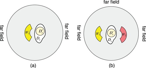
In this section, we present several numerical examples to support the abovementioned theoretical framework. We start from a simple control configuration as shown in Figure 2(a) with one near control region $W_1$. Then, we extend our numerical study into a multiple-region regime with two near field control regions $W_1$ and $W_2$ as sketched in Figure 2(b). The source and control regions are in free space. As we mentioned in Remark 2.1, the actual source $D_s$ can be arbitrarily shaped as long as it is Lipschitz and compactly embeds the fictitious source $D_s^{\mathrm{\prime }}$. In the following simulations, we use a spherical fictitious source $D_s^{\mathrm{\prime }}$, and its radius is 0.31 m centred at the origin. When we apply the Debye potential method, the source is modelled by 200×100 $\theta \varphi$-mesh. The EM fields are approximated using 70 harmonic orders, i.e. L = 70 in (11(11) $\{\begin{array}{l}{w}_u\left(\mathbf{y}\right)={\displaystyle \sum _{l=0}^L\sum _{p=-l}^l{\alpha }_{pl}{Y}_l^p\left(\hat{\mathbf{y}}\right),}\\ w_v\left(\mathbf{y}\right)={\displaystyle \sum _{l=0}^L\sum _{p=-l}^l{\text{β}}_{pl}{Y}_l^p\left(\hat{\mathbf{y}}\right),}\end{array}$(11) ), resulting in a total of 5041 unknown coefficients. While the source is discretized by 2808 triangle patches resulting in 4212 unknowns when the integral equation method. Subsections 3.1 and  3.2 discuss the performance of our strategy in each of the configurations mentioned above.

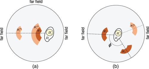
Figure 2. Sketch of the problem geometry showing the near control region(s) $W_1$ and/or $W_2$ and the source region $D_s$. (a) One control region. (b) Two control regions.

Before discussing the numerical examples, we shall introduce some measures to assess the control performance. In the following content, we use the relative or absolute $L^2$-norm error to evaluate the control accuracy of the proposed method. We use the relative error when the prescribed field is non-zero, otherwise we use the absolute error. The $L^2$-norm error, is defined as (26) $\Vert err{\Vert }_{L^2\left(\mathrm{\partial }{W}_j\right)}=\{\begin{array}{ll}{\displaystyle \frac{\Vert \mathbf{G}-\mathbf{P}{\Vert }_{L^2\left(\mathrm{\partial }{W}_j\right)}}{\Vert \mathbf{P}{\Vert }_{L^2\left(\mathrm{\partial }{W}_j\right)}}}& \mathrm{i}\mathrm{f}\Vert \mathbf{P}{\Vert }_{L^2\left(\mathrm{\partial }{W}_j\right)}\ne 0,\\ \Vert \mathbf{G}-\mathbf{P}{\Vert }_{L^2\left(\mathrm{\partial }{W}_j\right)}& \mathrm{i}\mathrm{f}\Vert \mathbf{P}{\Vert }_{L^2\left(\mathrm{\partial }{W}_j\right)}=0,\end{array}$(26) for each $j=\overline{1,2}$. $\mathbf{G}=\mathbf{A}{\mathbf{w}}_{\mathbf{d}}$ denotes the generated field, and $\mathbf{P}$ is prescribed field. $\mathbf{G}$ and $\mathbf{P}$ can be either $\mathbf{E}$ or $\mathbf{H}$. Such a $L^2$-norm error is an overall quantitative measure of control performance. Additionally, we define another measure to show the control accuracy in each mesh point, i.e. the pointwise error, (27) $er{r}_i=\{\begin{array}{ll}{\displaystyle \frac{|G_i-P_i|}{|P_i|}}& \mathrm{i}\mathrm{f}{P}_i\ne 0,\\ |G_i-P_i|& \mathrm{i}\mathrm{f}{P}_i=0,\end{array}$(27) where $er{r}_i$ is the relative or absolute error in the $i^{th}$ evaluation point.

Moreover, we define the radiated power and stored energy to determine the feasibility of the source. We can calculate the radiated power and stored energy via (28) $\begin{array}{r}{P}_{\mathrm{r}\mathrm{a}\mathrm{d}}=\mathfrak{R}\mathfrak{e}[{\int }_S\hat{\mathbf{n}}\cdot (\mathbf{E}\times {\mathbf{H}}^{\ast }\left)\mathrm{d}S\right],\end{array}$(28) (29) $\begin{array}{r}{P}_{\mathrm{s}\mathrm{t}\mathrm{o}\mathrm{r}}=\mathfrak{I}\mathfrak{m}[{\int }_S\hat{\mathbf{n}}\cdot (\mathbf{E}\times {\mathbf{H}}^{\ast }\left)\mathrm{d}S\right],\end{array}$(29) where $\hat{\mathbf{n}}$ is the unit vector normal to the source surface $\mathrm{\partial }{D}_s$, the power is defined by Poynting's theorem [45]. $\mathfrak{R}\mathfrak{e}$ and $\mathfrak{I}\mathfrak{m}$ respectively denotes the real and imaginary operator. The quality factor (Q) is a dimensionless parameter that describes the resonance behaviour of a harmonic source. It is defined by the radiated power and stored energy, as (30) $Q=\frac{2\pi \cdot P_{\mathrm{s}\mathrm{t}\mathrm{o}\mathrm{r}}}{P_{\mathrm{r}\mathrm{a}\mathrm{d}}}.$(30)

3.1. One near control region

Firstly, we consider a simple geometry with only one control region, as shown in Figure 2(a). The prescribed field in $W_1$ is a plane wave and the electric field is defined by $\mathbf{E}\left(\mathbf{r}\right)={\mathbf{E}}_{\mathbf{0}}{e}^{i\mathbf{k}\cdot \mathbf{r}}$, where ${\mathbf{E}}_{\mathbf{0}}=[0,1,0]$ and $\mathbf{k}=[-1,0,0]k$. The wavenumber k is 1, equivalently, $f=$ 47.75 MHz. The magnetic field can be attained by $\mathbf{H}\left(\mathbf{r}\right)=\frac{1}{\omega \mu }\mathbf{k}\times \mathbf{E}\left(\mathbf{r}\right)$. Note that the defined electric field in Cartesian coordinates indicates the EM wave propagates along $-\hat{\mathbf{x}}$ direction and electric field is polarized in $\hat{\mathbf{y}}$ direction. To ease the computation of spherical harmonics, we shall transform the EM fields from Cartesian coordinates into spherical coordinates via a rotation matrix [46] (see Appendix). The control region is an annular sector, and it is defined in the spherical coordinates (with respect to the origin) by (31) $W_1=\left\{\right(r,\theta ,\varphi ):r\in [0.5,0.55],\theta \in [\frac{\pi }{4},\frac{3\pi }{4}],\varphi \in [\frac{3\pi }{4},\frac{5\pi }{4}]\},$(31) where $W_1$ is discretized into 8000 collocation points on the surface. The $\mathbf{E}$ and $\mathbf{H}$ are evaluated at the discrete mesh points.

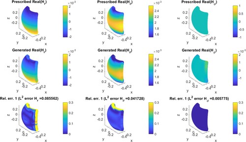
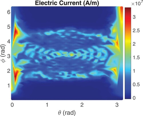
As we discussed in Section 2, two approaches are used in the forward modelling, and two regularization methods are applied to solve the inverse problem. Therefore, there are four available combinations in total to address the inverse source problem, i.e. ‘Debye potential with TSVD’, ‘Debye potential with Tikhonov’, ‘integral equation with TSVD’, and ‘integral equation with Tikhonov’. We shall test the performance of these possible methods. In the following, we present EM field control simulation results in one region. We show the results obtained by the ‘integral equation with TSVD’ method for an illustrative purpose. The prescribed and generated fields in the control region $W_1$ are shown in Figure 3 for electric field and Figure 4 for magnetic fields. The first row shows the three components of prescribed fields in each figure. The second row is the generated field by the inverted source. The third row is the relative pointwise error. Note that only the real part of the fields is considered here since the imaginary part exhibits similar results. We notice that the generated fields, either electric or magnetic, almost show the same pattern as the prescribed fields. The $L^2$-norm error of the electric field is of order ${10}^{-4}$, and it is ${10}^{-2}$ for the magnetic field. The less accuracy of the magnetic field is due to the unbalanced vector $\mathbf{b}$ in (20(20) $\mathbf{A}\mathbf{w}{}_d=\mathbf{b},$(20) ) that contains both $\mathbf{E}$ and $\mathbf{H}$ ($\mathbf{H}$ is about 377 times less than $\mathbf{E}$.)

Figure 3. Electric field ($\mathbf{E}$) synthesis in an exterior control region using the ‘integral equation with TSVD’.

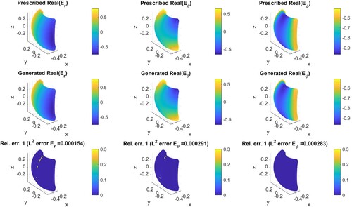
Figure 4. Magnetic field ($\mathbf{H}$) synthesis in an exterior control region using the ‘integral equation with TSVD’.

Furthermore, we also test the same control geometry using the other three methods. The pointwise errors are shown in Figure 5 for electric fields and Figure 6 for magnetic fields. Similarly, the three columns exhibit the three components of the electric or magnetic fields. Each row corresponds to one method.If we compare the first row with the third row and the second row with the fourth row, we can observe that the integral equation method generally outperforms the Debye potential method for both regularization methods. The lower accuracy of the Debye potential method is due to the imprecise calculation of the curl operator ($\mathrm{\nabla }\times$) in (15(15) $\{\begin{array}{l}{\mathbf{A}}_g\left(\mathbf{r}\right)=\mathrm{\nabla }\times (\mathrm{\nabla }\times u_g\mathbf{r})+k\mathrm{\nabla }\times v_g\mathbf{r},\\ {\mathbf{B}}_g\left(\mathbf{r}\right)=\mathrm{\nabla }\times (\mathrm{\nabla }\times v_g\mathbf{r})+k\mathrm{\nabla }\times u_g\mathbf{r}.\end{array}$(15) ). The Debye potential method uses the potentials u and v inversion to obtain the densities. Then we calculate the $\mathbf{E}$ and $\mathbf{H}$ fields from u and v in (15(15) $\{\begin{array}{l}{\mathbf{A}}_g\left(\mathbf{r}\right)=\mathrm{\nabla }\times (\mathrm{\nabla }\times u_g\mathbf{r})+k\mathrm{\nabla }\times v_g\mathbf{r},\\ {\mathbf{B}}_g\left(\mathbf{r}\right)=\mathrm{\nabla }\times (\mathrm{\nabla }\times v_g\mathbf{r})+k\mathrm{\nabla }\times u_g\mathbf{r}.\end{array}$(15) ). To avoid instabilities in the numerical calculation of the curl of the potentials, the addition theorem and the orthogonality of spherical harmonics were used in [29] to come up with a finite-sum approximation for u and v. This approximation was then used to calculate the curl and curl-curls necessary to get the $\mathbf{E}$ and $\mathbf{H}$ fields. However, the tiny numerical artifacts from the finite-sum approximation of the potentials got propagated in the supposed exact calculation of the curls since equation (4.10) of [29] requires the derivatives of the potentials. The loss of some orders of accuracy signals that more spherical harmonics and a significantly denser mesh are needed to make the Debye potential method more accurate. Regarding the selection of the regularization method, we shall compare the third row with the fourth row. We notice that the $L^2$-norm error of the TSVD method is about one order less than that of the Tikhonov regularization. This can be explained by the selection of an appropriate regularization parameter α in (24(24) ${\hat{\mathbf{w}}}_d=\underset{{\mathbf{w}}_d\in \mathrm{\partial }{D}_s}{\mathrm{a}\mathrm{r}\mathrm{g}\mathrm{m}\mathrm{i}\mathrm{n}}[\sum _{j=1}^2{\xi }_j\Vert \mathbf{A}{\mathbf{w}}_d-\mathbf{b}{\Vert }_{L^2\left(\mathrm{\partial }{W}_j\right)}^2+\alpha \Vert {\mathbf{w}}_d{\Vert }_{L^2\left(\mathrm{\partial }{D}_s^{\mathrm{\prime }}\right)}^2],$(24) ). Essentially, the Tikhonov regularized solution is the same as the solution obtained by the SVD if the regularization parameter α is sufficiently small (smaller than the smallest singular value) [43]. However, we truncate the SVD to remove the effects of minimal singular values that help to reduce oscillations in the solution [47]. In Tikhonov regularized solution, we notice the parameter α is about ${10}^{-19}$. The minimal value may cause fast oscillations in the solution. The inverted current on the source $\mathrm{\partial }{D}_s$ is shown in Figure 7 to demonstrate this phenomenon. The current is displayed in a 2D $(\varphi ,\theta )$-plane for a better perspective. Here, we only consider one current type, i.e. the electric current $\mathbf{J}$. In Figure 7, the first row shows the current computed by Debye potential method with two regularization methods. The second row displays the results of the integral equation method. We observe that the TSVD regularized solution is more stable. The ‘integral equation with TSVD’ method can produce the best solution among the four approaches regarding the control accuracy.

Figure 5. Pointwise relative error of electric field ($\mathbf{E}$) using four control strategies.

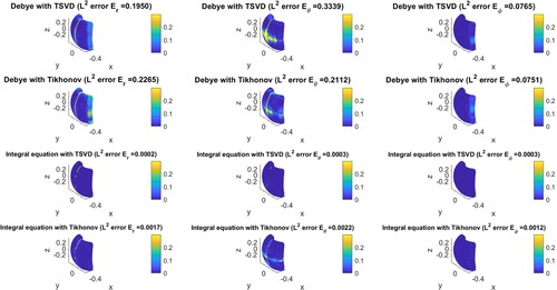
Figure 6. Pointwise relative error of magnetic field ($\mathbf{H}$) using four control strategies.

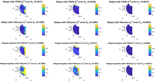
Figure 7. Inverted surface electric current ($\mathbf{J}$) on the source $\mathrm{\partial }{D}_s$. (a) ‘Debye potential with TSVD’ method. (b) ‘Debye potential with Tikhonov’ method. (c) ‘Integral equation with TSVD’ method. (d) ‘Integral equation with Tikhonov’ method.

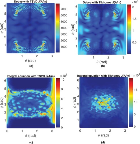
Furthermore, we also compare the power budget as well as the quality factor (Q) to determine the feasibility of the source. Table 1 lists the results of four approaches. It is worth noting that the Debye potential method can produce a source with remarkably low Q, indicating the source is almost non-oscillating. This unique feature is conducive to implementing the actual source. Besides, the integral equation method's radiated power is much higher than the Debye potential method, especially the ‘integral equation with TSVD’ method.

Table 1. Comparison of the power budget and Q among four approaches.

Method	Radiated power (dB)	Stored energy (dB)	Q
Debye with TSVD	95.56	93.01	3.5
Debye with Tikhonov	100.80	96.63	2.4
Integral equation with TSVD	143.9	175.2	8.5$\times {10}^3$
Integral equation with Tikhonov	104.9	130.0	2.1$\times {10}^3$

3.2. Two near control region

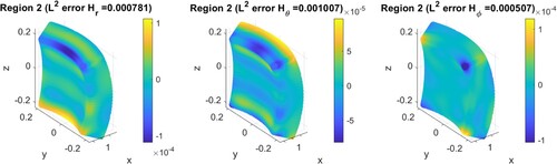
This subsection demonstrates the control strategy in a two-region regime. We show the performance of our scheme in creating the same plane EM wave given in 3.1 in $W_1$ and null field in $W_2$. The definition of $W_1$ is same as Subsection 3.1. $W_2$ is also an annular sector, and it is defined in spherical coordinate as (32) $W_2=\left\{\right(r,\theta ,\varphi ):r\in [0.5,0.6],\theta \in [\frac{3\pi }{8},\frac{5\pi }{8}],\varphi \in [-\frac{\pi }{8},\frac{\pi }{8}]\}+[0.5,0,0].$(32) Both $W_1$ and $W_2$ are discretized into 8000 collocation points. As the prescribed field in $W_2$ is zero; we shall only show the generated field for simplicity. Note that the generated field can also be regarded as the pointwise absolute error. The simulation results using the ‘integral equation with TSVD’ are shown in Figures 8–11. Compared with the one region control in Subsection 3.1, the generated fields $\mathbf{E}$ in Figure 8 and $\mathbf{H}$ in Figure 9 are almost the same, i.e. the same level of relative error. The $L^2$-norm error is ${10}^{-4}$ of electric field and ${10}^{-2}$ of the magnetic field, which indicates a good control in $W_1$. Regarding the second region $W_2$, the maximum amplitude of the generated field is of order ${10}^{-4}$, as shown in Figures 10 and 11. The $L^2$-norm errors are low with order ${10}^{-3}$ in $W_2$. In this simulation, good controls are observed in both $W_1$ and $W_2$. This suggests that our method can maintain a quiet region while producing a plane wave in the other region. This is known as the ‘contrast control’.

Figure 8. Electric field ($\mathbf{E}$) synthesis in an $W_1$ using the ‘integral equation with TSVD’.

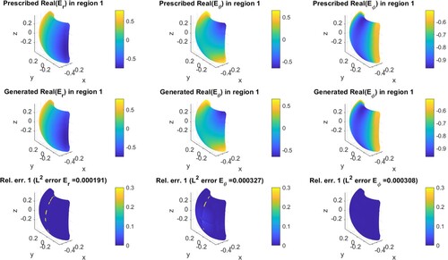
Figure 9. Magnetic field ($\mathbf{H}$) synthesis in an $W_1$ using the ‘integral equation with TSVD’.

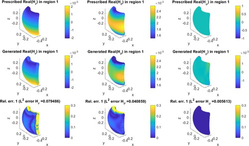
Figure 10. Generated electric field ($\mathbf{E}$) in an $W_2$ using the ‘integral equation with TSVD’.

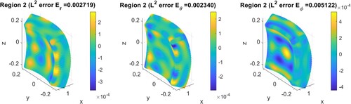
Figure 11. Generated magnetic field ($\mathbf{H}$) in an $W_2$ using the ‘integral equation with TSVD’.

The surface current $\mathbf{J}$ is also displayed in a 2D $(\varphi ,\theta )$-plane, in Figure 12. We find the distribution is similar to that in Figure 7(c). The magnitude of $\mathbf{J}$ is slightly larger, revealing that more control efforts are required to maintain the null region while producing a plane wave in the other region.

Figure 12. Inverted surface electric current ($\mathbf{J}$) on the source $\mathrm{\partial }{D}_s$.

4. Sensitivity analysis in free space

The previous section presents the EM field manipulation simulation results in one and two exterior regions. A plane wave is prescribed in the one-region control. The contrast control, i.e. one plane wave region and one null field region is implemented in the two-region regime. The $L^2$-norm error evaluates the control performance. The presented results back up the analysis of  [29] and show that our strategy works for each of the two configurations depicted in Figure 2. This section presents the sensitivity study for both ‘integral equation with TSVD’ and ‘Debye potential with TSVD’ methods. Based on the observations in Subsection 3.1, the ‘integral equation with TSVD’ method allows more accurate control. However, it requires high power and oscillates. The source obtained by the ‘Debye potential with TSVD’ method is more feasible than the integral equation method, i.e. less oscillating, but it sacrifices the control accuracy. In the following simulations, we aim to study the sensitivity of our strategy concerning variations in several physically relevant parameters, such as wavenumber k, the distance between the control region and the source, the control region size and, the mutual distance between the control regions (in the case of two control regions Figure 2(b)). The sensitivity study gives insight into the feasibility of implementing the physical source.

The geometry in the sensitivity analysis is depicted in Figure 13. To distinguish the original region (dark), the regions with modified parameters are shown in a light colour. For instance, $W_1^{\ast 2}$ denotes the near control, which is shifted away from the source, in which the superscript ‘2’ corresponds to the experiment number in Section 4.2.

Figure 13. Sketch of the geometry in sensitivity analysis. $W_1$ and $W_2$ are original near controls and they are shown in dark colour. The light-coloured regions with $W_1^{\ast n}$, where n = 2, 3 and 4, are corresponding to the experiments in Sections 4.2–4.4.

Remark 4.1

As noted in Subsection 3.1, for the Debye potential approach to yield accurate results, a very dense discretization of the control regions and more spherical harmonics are required. In [29], the authors were able to get very accurate results for a smaller geometry, a source that has radius 0.0105 m and control regions with thickness 0.04 m. They used 70 harmonic orders and 37800 collocation points on each control region. As this study aims to look at the feasibility of the proposed schemes, the dimensions of the source and control regions were chosen to represent practically relevant scenarios. Hence, the larger geometry: a source of radius 0.31 m and control regions of thickness 0.05 m and 0.1 m. In this study, we were constrained to limit the collocation points to N = 8000 on each control region as the integral equation approach will require a system with $6N$ (or $12N$ for the case of two control regions) equations, compared to the Debye potential approach which will result to two independent systems with just N (or $2N$) equations each. Proportionally choosing N to match the Debye potential results in [29] is computationally expensive. We will see in the results below that the Debye potential approach produced some results with low accuracy. However, the mathematical analysis in [29] guarantees that such results will be improved by using more collocation points and harmonic orders.

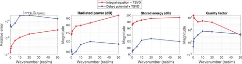
4.1. Varying the wavenumber k

We start by a simple geometry in Figure 2(a), where only one control region $W_1$ is considered. The region size is defined in (31(31) $W_1=\left\{\right(r,\theta ,\varphi ):r\in [0.5,0.55],\theta \in [\frac{\pi }{4},\frac{3\pi }{4}],\varphi \in [\frac{3\pi }{4},\frac{5\pi }{4}]\},$(31) ). The prescribed field in $W_1$ is the plane wave $\mathbf{E}\left(\mathbf{r}\right)=\hat{\mathbf{y}}{e}^{-ikx}$. In this simulation, we let the wavenumber vary from 0.1 rad m${}^{-1}$ to 50 rad m${}^{-1}$. The corresponding frequency varies from 4.775 MHz to 2.387 GHz. Only the wavenumber is changed in each simulation, and other parameters are fixed. The simulation results are shown in Figure 14. From left to right, four subplots respectively show the $L^2$-norm error of the radial component of electric field (${\mathbf{E}}_r$), radiated power by $D_s$, stored energy in $D_s$, and quality factor for both ‘integral equation with TSVD’ and ‘Debye potential with TSVD’ methods. For ‘integral equation with TSVD’ method, the $L^2$-norm error increases from ${10}^{-4}$ to ${10}^{-1}$ as the wavenumber increases. However, the $L^2$-norm error evaluating the ‘Debye potential with TSVD’ method is much worse, which exceeds 0.5 as long as the wavenumber is larger than 5. The radiated power and stored energy for both methods change similarly as the wavenumber increases, except for the opposite trend after 20 rad m${}^{-1}$. This suggests that the source obtained by the ‘integral equation with TSVD’ method is more energy-intensive at high frequencies. The ‘Debye potential with TSVD’ method can work at higher frequencies. The quality factor obtained from the ‘integral equation with TSVD’ method decrease along with the wavenumber increase, resulting in a less oscillating source. However, the ‘Debye potential with TSVD’ method produces the exact opposite change, indicating the source is more oscillating than the integral equation method. But the quality factor is in general much less than that produced by the ‘integral equation with TSVD’ method.

Figure 14. Results showing the control accuracy and the power budget varying with k. From left to right, (1) $L^2$-norm error of ${\mathbf{E}}_r$. (2) Radiated power by $D_s$. (3) Stored energy in $D_s$. (4) Quality factor.

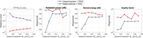
4.2. Varying the distance between the near control region and the source

The following results show the effect of variations in the distance between the near control region and the source. We still use the initial model in Figure 2(a). The near control $W_1$ is shifted further away from the source ($W_1^{\ast 2}$ in Figure 13(a)) while all other parameters are fixed. Note that the prescribed plane wave in $W_1$ is the same as that in Subsection 3.1. We define the distance as the spacing between the inner boundary of the annular sector and the boundary of the source. The investigated range of the distance is from 0.1 m to 0.7 m. The results are depicted in Figure 15. We notice that the control accuracy changes reversely for the two methods. In the ‘integral equation with TSVD’ method, the relative error in the near region increases when the control region moves further away from the source. In contrast, the relative error keeps on descending for the ‘Debye potential with TSVD’ method. In the entire range of distance, the integral equation method maintains the relative error within an order of ${10}^{-3}$. Though the Debye potential method realizes a high-accurate control at a more considerable distance, the relative error is still larger than ${10}^{-2}$. The power budget (radiated power and stored energy) and quality factor given by the Debye potential method shows a significant jump when the control region is pushed far away until the distance exceeds a threshold, 0.3 m. After the threshold, the power budget is comparable to the integral equation method. These changes suggest that the ‘integral equation with TSVD’ method can manipulate the EM fields in an exterior region that is well-separated from the source, even though more control effort is required to achieve good accuracy in control regions further from the source. However, the ‘Debye potential with TSVD’ method has the limitation to control the far region as the power budget and the quality factor changes significantly.

Figure 15. Results showing the control accuracy and the power budget varying with mutual distance between the control region and the source. From left to right, (1) $L^2$-norm error of ${\mathbf{E}}_r$. (2) Radiated power by $D_s$. (3) Stored energy in $D_s$. (4) Quality factor.

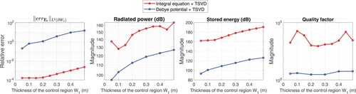
4.3. Varying the near control region size

In this subsection, we consider the behaviour of the control accuracy and the power budget concerning incremental increase in the outer radius of the near control region $W_1$ ($W_1^{\ast 3}$ in Figure 13(a)) with all the other parameters fixed. The increase of the outer radius is equivalent to enlarging the size of the control region. We shall use the thickness of the control region as the size indicator. The thickness is the difference between the outer radius and the inner radius of the annular sector. Following the same procedure in the previous study, the prescribed plane wave in $W_1$ is the same as that in Subsection 3.1. In this simulation, the inner radius of the control region is 0.5 m. The outer radius varies from 0.55 m to 1 m, i.e. the thickness varies from 0.05 m to 0.5 m. The maximum thickness of the control region is close to the diameter of the source. The results are shown in Figure 16. We notice that both the integral equation method and the Debye potential method change in the same way, i.e. the control accuracy and power budget keep worsening as the control region becomes large. This indicates it is difficult to control a large region, especially larger than the source. The quality factor does not change significantly in the entire range of the thickness.

Figure 16. Results showing the control accuracy and the power budget varying with the size of the control region. From left to right, (1) $L^2$-norm error of ${\mathbf{E}}_r$. (2) Radiated power by $D_s$. (3) Stored energy in $D_s$. (4) Quality factor.

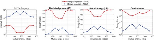
4.4. Varying the mutual distance between the near control regions

This sensitivity test considers two near control regions and varies the mutual distance. The first control region $W_1$ is prescribed as a plane wave, and the second region $W_2$ is null. In Figure 13(b), $W_1$ is fixed and we rotate $W_2$ around $D_s$ to obtain a new secondary control region $W_2^{\ast 4}$. The mutual angle ϕ determines the mutual distance between the two near controls as shown in Figure 13(b). The control accuracy and power budget are calculated as the angle ϕ varies from 0${}^{\circ }$ to 360${}^{\circ }$. If $\varphi =0^{\circ }$, the second control region $W_2$ is situated exactly behind the first control region, then it is rotated counterclockwise as ϕ increases, and finally, it is back to the starting point when $\varphi ={360}^{\circ }$. In this study, the prescribed plane wave in $W_1$ and null field in $W_2$ are the same as that in Subsection 3.2. The results are shown in Figure 17. We notice the curves for both methods are symmetric due to the symmetry of the relative position between the control region and the source. In the first subplot, the $L^2$-norm relative error of the integral equation method is less than ${10}^{-3}$ when ϕ is in the range of $[{90}^{\circ },{270}^{\circ }]$. If ϕ is out of this range, i.e. the near controls are too close to each other, the relative error, as well as the source power, becomes excessive. However, the Debye potential method shows opposite variations with respect to the mutual angle, e.g. the relative error is large in the range of $[{90}^{\circ },{270}^{\circ }]$. This is due to the relative distance being larger when the angle increases, and then the distance is shorter when the angle exceeds ${180}^{\circ }$. This indicates that the Debye potential method is limited to controlling the region far from the source. This phenomenon is investigated in Subsection 4.2. On the other hand, the Debye potential method gives a much worse $L^2$-norm error (even larger than 1). However, the power budget is much less than the integral equation method. This is observed in Subsection 3.1, i.e. the Debye potential method gives a low-power and less-oscillating source but loses the control accuracy. In this simulation, the control regions cannot be too close; otherwise, the accurate control effects are degraded using the integral equation method. However, the mutual distance between two control regions must be within a threshold when the Debye potential method is considered.

Figure 17. Results showing the control accuracy and the power budget varying with the mutual distance between two control regions. From left to right, (1) $L^2$-norm error of ${\mathbf{E}}_r$. (2) Radiated power by $D_s$. (3) Stored energy in $D_s$. (4) Quality factor.

5. Conclusions

This paper presents the sensitivity of the active manipulation of electromagnetic fields in free space. We demonstrate the existence of a current source (modeled as surface electric and/or magnetic current) such that it is capable of approximating a priori given field in some near control regions. We build upon our previous works and illustrate two approaches for forward modelling and two regularization methods for inversion. In other words, four combined approaches are demonstrated to solve the electromagnetic inverse source problem. We compare the performance of these four approaches using a baseline model where only one control region is considered. The simulation results suggest that the ‘integral equation with TSVD’ method can realize the best control accuracy but gives a high-power and oscillating source. The ‘Debye potential with TSVD’ method can achieve low-power source reconstruction whereas with the price paid for low control accuracy. Hence, we apply the ‘Debye potential with TSVD’ method and the ‘integral equation with TSVD’ method to perform the sensitivity study. We explored the behaviour of physically relevant parameters (power budget, control accuracy, and quality factor) concerning variations in the frequency, outward shift, the near control's outer radius, and the mutual distance between near controls.

In our simulations, we consider two initial models as shown in Figure 2. The first one contains one near control and the second one has two near control regions. In this paper, the prescribed field is a plane wave with only one control region. The plane wave is prescribed in one region in the two-region regime, and a null field is maintained in the other region. This is as known as ‘EM contrast control’. The simulation results in both of two control regimes show the $L^2$-norm error is within ${10}^{-3}$, which indicates a good accuracy level.

In addition, we performed the sensitivity study based on our initial model. In the geometry shown in Figure 2(a), the operating frequency first varies while all other parameters are fixed. The frequency is swept from 4.775 MHz to 2.387 GHz (k is from 0.1 to 50). We observe the fast and significant increase of the $L^2$-norm error and power budget for both methods. The quality factor changes reversely for the two methods. These changes indicate that the integral equation method is limited to manipulating the high-frequency EM fields using a relatively large source (Its diameter is five times as large as the wavelength). However, this limitation is not obvious for Debye potential method.

In the second simulation, the near control region is moved outward. We noticed that the ‘integral equation with TSVD’ method can manipulate the EM fields in an exterior region that is well-separated from the source, even though more power is required to achieve good accuracy in control regions further from the source. However, the ‘Debye potential with TSVD’ method cannot control the far region as the power budget and the quality factor increase fast, suggesting the source is power-intensive and oscillating when controlling the EM fields in the outlying area.

Next, we vary the outer radius of the near control region to explore the effect of the near region's size on the control accuracy and power budget. The relative error and power budget change in the same way for both approaches. The control accuracy worsens as the control region enlarges. The quality factor does not change significantly. The simulation results show that the active control scheme requires more effort to achieve accurate EM field control on a bigger region. We also considered the geometry in Figure 2(b). We rotate the second near control region around the source in the simulation. We arrive at the opposite conclusion using the integral equation and Debye potential methods. The integral equation method can realize good control accuracy within $3\times {10}^{-3}$ as long as the two near control regions are separated by an angle $\varphi \in [{90}^{\circ },{270}^{\circ }]$. However, outside this range, the control performance is gradually degrading. This means two regions have to be well-separated. On the contrary, the Debye potential method is limited to controlling the region that should not be far away from the source. When $W_1$ is rotated by an angle, the control accuracy degrades. Nevertheless, the control accuracy of the Debye potential method is generally worse than the integral equation method.

Disclosure statement

The authors claim that there is no potential conflict of interest.

Additional information

Funding

J. Chen and C. Qi would like to acknowledge the National Science Foundation (NSF), USA for funding their work [award number 1801925]. D. Onofrei and N. J. A. Egarguin would like to acknowledge the Army Research Office, USA for funding their work [award number W911NF-17-1-0478].

Appendices

Appendix 1. Debye potential method

Appendix 2. Integral equation method

References

- Chen A, Monticone F. Active scattering-cancellation cloaking: broadband invisibility and stability constraints. IEEE Trans Antennas Propag. 2019;68:1655–1664.
- Bisht MS, Srivastava KV. Controlling electromagnetic scattering of a cylindrical obstacle using concentric array of current sources. IEEE Trans Antennas Propag. 2020;68:8044–8052.
- Mitri F. Active electromagnetic invisibility cloaking and radiation force cancellation. J Quant Spectrosc Radiat Transf. 2018;207:48–53.
- Norris AN, Amirkulova FA, Parnell WJ. Source amplitudes for active exterior cloaking. Inverse Probl. 2012;28:105002.
- Kwon DH. Lossless tensor surface electromagnetic cloaking for large objects in free space. Phys Rev B. 2018;98:125137.
- Selvanayagam M, Eleftheriades GV. An active electromagnetic cloak using the equivalence principle. IEEE Antennas Wirel Propag Lett. 2012;11:1226–1229.
- Sengupta S, Council H, Jackson DR, et al. Active radar cross section reduction of an object using microstrip antennas. Radio Sci. 2020;55:1–20.
- Onofrei D. On the active manipulation of fields and applications: I. the quasistatic case. Inverse Probl. 2012;28:105009.
- Brown T, Narendra C, Vahabzadeh Y, et al. On the use of electromagnetic inversion for metasurface design. IEEE Trans Antennas Propag. 2019;68:1812–1824.
- Pang Y, Mo M, Li Y, et al. Dynamically controlling electromagnetic reflection using reconfigurable water-based metasurfaces. Smart Mater Struct. 2020;29:115018.
- Luo XY, Guo WL, Chen K, et al. Active cylindrical metasurface with spatial reconfigurability for tunable backward scattering reduction. IEEE Trans Antennas Propag. 2020;69:3332–3340.
- Zhu BO, Chen K, Jia N, et al. Dynamic control of electromagnetic wave propagation with the equivalent principle inspired tunable metasurface. Sci Rep. 2014;4:1–7.
- Huang C, Zhang C, Yang J, et al. Reconfigurable metasurface for multifunctional control of electromagnetic waves. Adv Opt Mater. 2017;5:1700485.
- Ma Q, Hong QR, Bai GD, et al. Editing arbitrarily linear polarizations using programmable metasurface. Phys Rev Appl. 2020;13:021003.
- Ayestarán RG, León G, Pino MR, et al. Wireless power transfer through simultaneous near-field focusing and far-field synthesis. IEEE Trans Antennas Propag. 2019;67:5623–5633.
- Clauzier S, Mikki SM, Antar YM. Design of near-field synthesis arrays through global optimization. IEEE Trans Antennas Propag. 2014;63:151–165.
- Xiao JJ, Nehorai A. Optimal polarized beampattern synthesis using a vector antenna array. IEEE Trans Signal Process. 2008;57:576–587.
- Wu JW, Wu RY, Bo XC, et al. Synthesis algorithm for near-field power pattern control and its experimental verification via metasurfaces. IEEE Trans Antennas Propag. 2018;67:1073–1083.
- Gao F, Zhang F, Wakatsuchi H, et al. Synthesis and design of programmable subwavelength coil array for near-field manipulation. IEEE Trans Microw Theory Tech. 2015;63:2971–2982.
- Lopéz YA, Andrés FLH, Pino MR, et al. An improved super-resolution source reconstruction method. IEEE Trans Instrum Meas. 2009;58:3855–3866.
- Quijano JLA, Vecchi G. Improved-accuracy source reconstruction on arbitrary 3-d surfaces. IEEE Antennas Wirel Propag Lett. 2009;8:1046–1049.
- Álvarez Y, Las-Heras F, Pino MR. Reconstruction of equivalent currents distribution over arbitrary three-dimensional surfaces based on integral equation algorithms. IEEE Trans Antennas Propag. 2007;55:3460–3468.
- Angell TS, Kirsch A. Optimization methods in electromagnetic radiation. New York: Springer Science & Business Media; 2004.
- Egarguin NJA, Onofrei D, Platt E. Sensitivity analysis for the active manipulation of helmholtz fields in 3d. Inverse Probl Sci Eng. 2020;28:314–339.
- Onofrei D, Platt E. On the synthesis of acoustic sources with controllable near fields. Wave Motion. 2018;77:12–27.
- Onofrei D. Active manipulation of fields modeled by the helmholtz equation. J Int Equ Appl. 2014;26:553–572.
- Qi C, Egarguin NJA, Onofrei D, et al. Feasibility analysis for active near/far field acoustic pattern synthesis in free space and shallow water environments. Acta Acust. 2021;5:39.
- Egarguin NJA, Onofrei D, Qi C, et al. Active manipulation of helmholtz scalar fields in an ocean of two homogeneous layers of constant depth. Inverse Probl Sci Eng. 2021;29(13):1–25.
- Onofrei D, Platt E, Egarguin NJA. Active manipulation of exterior electromagnetic fields by using surface sources. Q Appl Math. 2020;78:641–670.
- Marengo EA, Devaney AJ. The inverse source problem of electromagnetics: linear inversion formulation and minimum energy solution. IEEE Trans Antennas Propag. 1999;47:410–412.
- Marengo EA, Ziolkowski RW. Nonradiating and minimum energy sources and their fields: generalized source inversion theory and applications. IEEE Trans Antennas Propag. 2000;48:1553–1562.
- Mohajer M, Safavi-Naeini S, Chaudhuri SK. Surface current source reconstruction for given radiated electromagnetic fields. IEEE Trans Antennas Propag. 2009;58:432–439.
- Qi C, Chen J, Egarguin NJA, et al. Feasibility analysis for active manipulation of electromagnetic fields in free space. IEEE International Symposium on Antennas and Propagation and USNC-URSI Radio Science Meeting (APS/URSI). Singapore: IEEE; 2021, p. 1841–1842.
- Egarguin NJA, Zeng S, Onofrei D, et al. Active control of helmholtz fields in 3d using an array of sources. Wave Motion. 2020;94:102523.
- Colton D, Kress R. Integral equation methods in scattering theory. Philadelphia: SIAM; 2013.
- Smyshlyaev VP. The high-frequency diffraction of electromagnetic waves by cones of arbitrary cross sections. SIAM J Appl Math. 1993;53:670–688.
- Rowe E. Decomposition of vector fields by scalar potentials. J Phys A Math Gen. 1979;12:145.
- O'Neil M. A generalized debye source approach to electromagnetic scattering in layered media. J Math Phys. 2014;55:012901.
- Wilcox CH. Debye potentials. J Math Mech. 1957;6:167–201.
- Colton DL, Kress R, Kress R. Inverse acoustic and electromagnetic scattering theory. Vol. 93. New York: Springer; 1998.
- Rao S, Wilton D, Glisson A. Electromagnetic scattering by surfaces of arbitrary shape. IEEE Trans Antennas Propag. 1982;30:409–418.
- Nikolova NK. Introduction to microwave imaging. Cambridge: Cambridge University Press; 2017.
- Mueller JL, Siltanen S. Linear and nonlinear inverse problems with practical applications. Philadelphia: SIAM; 2012.
- Bonesky T. Morozov's discrepancy principle and tikhonov-type functionals. Inverse Probl. 2008;25:015015.
- Pozar DM. Microwave engineering. New York: John Wiley & Sons; 2011.
- Balanis CA. Antenna theory: analysis and design. New York: John Wiley & Sons; 2015.
- Rodriguez JAO Regularization methods for inverse problems. Minneapolis: University of Minnesota; 2011.