Solving Lane–Emden equations with boundary conditions of various types using high-order compact finite differences

Abstract

In this study, a high-order compact finite difference method is used to solve Lane–Emden equations with various boundary conditions. The norm is to use a first-order finite difference scheme to approximate Neumann and Robin boundary conditions, but that compromises the accuracy of the entire scheme. As a result, new higher-order finite difference schemes for approximating Robin boundary conditions are developed in this work. We test the applicability and performance of the method using different examples of Lane–Emden equations. Convergence analysis is provided, and it is consistent with the numerical results. The results are compared with the exact solutions and published results from other methods. The method produces highly accurate results, which are displayed in tables and graphs.

Keywords:

• Lane–Emden equations
• boundary value problems
• compact finite differences
• quasilinearization

Mathematics Subject Classifications (2010):

• 65L10
• 65L12
• 34B15

1. Introduction

Lane–Emden equations model a wide range of problems in physics and astrophysics, with applications including stellar structure, thermal explosions, isothermal gas spheres, radiative cooling, thermionic currents, and the thermal behaviour of a spherical cloud of gas [1–8]. They are singular ordinary differential equations first studied by astrophysicist Jonathan Homer Lane [9]. He later collaborated with Robert Emden to investigate them further. They considered the thermal behaviour of a spherical cloud of gas acting under the mutual attraction of its molecules and subject to the classical laws of thermodynamics. Due to these important applications, the Lane–Emden equation is among the most numerically investigated differential equations. One of the challenges with solving them is dealing with the singularity at x = 0. The Lane–Emden equations have been solved using various analytical and numerical methods, such as Adomian decomposition method [10–13], variational iterational method [14–17], Taylor series method [18], differential transformation method [19], modified Homotopy analysis method [20], finite difference method [21–23], spline method [24–27], the optimal iteration method [28], Adomaian decomposition method with Green's function [29,30], Chebyshev economization method [31], optimal homotopy analysis method [32], Haar wavelet collocation method [33], Sin-Galerkin method [34], differential transform method [35], homotopy perturbation method [36], asymptotic method [37], Bernstein polynomials method [38], to name a few.

Compact finite difference schemes (CFDS) have gained popularity in numerical approximations in recent years. Lele [39] gave an in-depth description of CFDS for various applications such as interpolation, filtering, and evaluating derivatives. The CFDS has been applied to solve differential equations such as Poisson's equation [40], Burger's equation [41,42], American option pricing problems [43], Navier–Stokes equation [44], integro-differential equation [45,46], Korteweg–de Vries equation [47], Black–Scholes equation [48,49], dynamical systems [50,51], and many more [52–56]. Their main advantage is that, with few grid points, they attain very high order accuracy.

In this paper, we use higher-order compact finite difference schemes to solve Lane–Emden equations of the form: (1) $y^{\mathrm{\prime }\mathrm{\prime }}(x)+\frac{\alpha }{x}{y}^{\mathrm{\prime }}(x)=f(x,y)\mathrm{for}0\le x\le 1,$(1) subject to the boundary conditions $\begin{array}{rl}y(0)& ={\alpha }_1,y(1)={\beta }_1,\\ y^{\mathrm{\prime }}(0)& ={\alpha }_2,y^{\mathrm{\prime }}(1)={\beta }_2,\\ y^{\mathrm{\prime }}(0)& ={\gamma }_1,{\alpha }_{3}y(1)+{\beta }_3{y}^{\mathrm{\prime }}(1)={\gamma }_2,\end{array}$where $\alpha ,{\alpha }_1,{\alpha }_2,{\alpha }_3,{\beta }_1,{\beta }_2,{\beta }_3,{\gamma }_1,{\gamma }_2$ are constants. We assume the following conditions on $f(x,y)$:

• $f(x,y),f_y(x,y)\in C(\mathrm{\Omega })$,

• $f_y(x,y)\ge 0$ on Ω, where $\mathrm{\Omega }:=\{(0,1]\times \mathbb{R}\}$.

To maintain the same level of accuracy at the boundary points as in the interior points, the compact finite schemes are adjusted at the boundaries. In this work, we develop new compact schemes for Robin boundary conditions. In most cases, Neumann or Robin boundary conditions are approximated using first-order schemes, even if a higher-order method is used to solve the equation. The disadvantage is that the accuracy of the whole method is affected. To deal with the singularity at x = 0, we apply L‘Hospital‘s rule [27] to Equation (1(1) $y^{\mathrm{\prime }\mathrm{\prime }}(x)+\frac{\alpha }{x}{y}^{\mathrm{\prime }}(x)=f(x,y)\mathrm{for}0\le x\le 1,$(1) ). Thus, Equation (1(1) $y^{\mathrm{\prime }\mathrm{\prime }}(x)+\frac{\alpha }{x}{y}^{\mathrm{\prime }}(x)=f(x,y)\mathrm{for}0\le x\le 1,$(1) ) reduces to (2) $y^{\mathrm{\prime }\mathrm{\prime }}+U(x)y^{\mathrm{\prime }}=G(x,y),$(2) where $G(x,y)=\{\begin{array}{ll}f(x,y),& \text{if }x\ne 0,\\ \frac{1}{\alpha +1}f(x,y),& \text{if }x=0,\end{array}$and $U(x)=\{\begin{array}{ll}\frac{\alpha }{x},& \text{if }x\ne 0,\\ 0,& \text{if }x=0.\end{array}$The rest of the paper is laid out as follows. In Section 2, we discuss the quasilinearization technique. In Section 3, we present the derivations of the sixth-order compact finite difference schemes. In Section 4, we discuss the development of compact finite difference schemes with various boundary conditions. We discuss the convergence of the method in Section 5. The results and discussion are presented in Section 6, followed by the conclusions in Section 7.

2. Quasilinearization

Before applying the CFDS, we must first linearize Equation (2(2) $y^{\mathrm{\prime }\mathrm{\prime }}+U(x)y^{\mathrm{\prime }}=G(x,y),$(2) ). To this end, we use the quasilinearization (QLM) technique that Bellman and Kalaba introduced [57]. The QLM reduces the nonlinear Lane–Emden equations into a sequence of linear Lane–Emden equations, which we solve iteratively until a set tolerance level is reached. One of the key factors motivating many academics to employ the quasilinearization method is its quadratic convergence and numerical stability [58]. In [59], Keller discusses the method's stability and convergence properties.

We expand the nonlinear function $G(x,y)$ in Equation (2(2) $y^{\mathrm{\prime }\mathrm{\prime }}+U(x)y^{\mathrm{\prime }}=G(x,y),$(2) ) using Taylor's series up to the first-order terms to get (3) $\begin{array}{rl}& y_{r+1}^{″}+U(x)y_{r+1}^{\prime }=G(x,y_r)+(y_{r+1}-y_r)\frac{\mathrm{\partial }G(x,y_r)}{\mathrm{\partial }{y}_r}\end{array}$(3) (4) $\begin{array}{rl}& y_{r+1}^{\mathrm{\prime }\mathrm{\prime }}+a_1{y}_{r+1}^{\mathrm{\prime }}+a_0{y}_{r+1}=R(x,y_r)\end{array}$(4) where $\begin{array}{rl}{a}_0& =-\frac{\mathrm{\partial }G(x,y_r)}{\mathrm{\partial }{y}_r}\\ a_1& =U(x)\\ R(x,y_r)& =G(x,y_r)+a_0{y}_r\end{array}$

3. Compact finite difference schemes at interior nodes

In this section, we present the derivations of the sixth-order CFDS for approximating first and second derivatives. We consider a function $f(x)$ defined on $x\in [a,b]$, where a and b are arbitrary constants. We discretize the domain into N number of nodes with a uniform step size $h=(b-a)/(N-1)$ and nodes $x_i=a+ih,0\le i\le N-1.$

3.1. First derivative approximation

The general formula for approximating the first derivatives is given by (5) $A{f}_{i-1}^{\mathrm{\prime }}+f_i^{\mathrm{\prime }}+A{f}_{i+1}^{\mathrm{\prime }}=a_1{f}_{i-2}+a_2{f}_{i-1}+a_3{f}_i+a_4{f}_{i+1}+a_5{f}_{i+2}+T_1,$(5) where $f_i=f(x_i)$ and $T_1$ is the truncation error. $A,a_i(i=1,\dots 5)$ are constants to be determined. The values of these constants are obtained by expanding both sides of Equation (5(5) $A{f}_{i-1}^{\mathrm{\prime }}+f_i^{\mathrm{\prime }}+A{f}_{i+1}^{\mathrm{\prime }}=a_1{f}_{i-2}+a_2{f}_{i-1}+a_3{f}_i+a_4{f}_{i+1}+a_5{f}_{i+2}+T_1,$(5) ) using the Taylor series expansion about $x_i$ and matching the coefficients of $f_i^{(n)}$, with $n=1,2,\dots ,6$ for a sixth-order accurate scheme. That results in six algebraic equations that are solved to obtain the following constants: $A=\frac{1}{3},a_1=-\frac{1}{36h},a_2=-\frac{7}{9h},a_3=0,a_4=\frac{7}{9h},a_5=\frac{1}{36h}.$Therefore, the scheme for approximating the first derivative is given by (6) $\frac{1}{3}{f}_{i-1}^{\prime }+f_i^{\prime }+\frac{1}{3}{f}_{i+1}^{\prime }=-\frac{1}{36h}{f}_{i-2}-\frac{7}{9h}{f}_{i-1}+\frac{7}{9h}{f}_{i+1}+\frac{1}{36h}{f}_{i+2}+T_1^{(i)}.$(6) The first unmatched coefficients of Taylor series expansion are used to determine the truncation error, which is given by $T_1^{(i)}=\frac{h^7}{5040}(128a_1{f}^{(7)}(x)+a_2{f}^{(7)}(x)-a_4{f}^{(7)}(x)-128a_5{f}^{(7)}(x))=-\frac{h^6}{1260}{f}^{(7)}(x).$

3.2. Second derivative approximation

The general formula for approximating second derivatives is given by (7) $A{f}_{i-1}^{\mathrm{\prime }\mathrm{\prime }}+f_i^{\mathrm{\prime }\mathrm{\prime }}+A{f}_{i+1}^{\mathrm{\prime }\mathrm{\prime }}=a_1{f}_{i-2}+a_2{f}_{i-1}+a_3{f}_i+a_4{f}_{i+1}+a_5{f}_{i+2}+T_2,$(7) with $T_2$ being the truncation error. Similarly, the values of these constants are obtained by expanding both sides of Equation (7(7) $A{f}_{i-1}^{\mathrm{\prime }\mathrm{\prime }}+f_i^{\mathrm{\prime }\mathrm{\prime }}+A{f}_{i+1}^{\mathrm{\prime }\mathrm{\prime }}=a_1{f}_{i-2}+a_2{f}_{i-1}+a_3{f}_i+a_4{f}_{i+1}+a_5{f}_{i+2}+T_2,$(7) ) using the Taylor series expansion about $x_i$ and matching the coefficients of $f_i^{(n)}$, with $n=1,2,\dots ,6$ for a sixth-order accurate scheme. That results in six algebraic equations that are solved to obtain the following constants. $A=\frac{2}{11},a_1=\frac{3}{44h^2},a_2=\frac{12}{11h^2},a_3=-\frac{51}{22h^2},a_4=\frac{12}{11h^2},a_5=\frac{3}{44h^2}.$Therefore, the scheme for approximating the second derivative is given by (8) $\begin{array}{r}\frac{2}{11}{f}_{i-1}^{″}+f_i^{″}+\frac{2}{11}{f}_{i+1}^{″}=\frac{3}{44h^2}{f}_{i-2}+\frac{12}{11h^2}{f}_{i-1}-\frac{51}{22h^2}{f}_i+\frac{12}{11h^2}{f}_{i+1}+\frac{3}{44h^2}{f}_{i+2}+T_2^{(i)}.\end{array}$(8) Similarly, the first unmatched coefficients of Taylor series expansion are used to determine the truncation error, which is given by $T_2=\frac{h^8}{40320}(-256a_1{f}^{(8)}(x)-a_2{f}^{(8)}(x)-a_4{f}^{(8)}(x)-256a_5{f}^{(8)}(x))=-\frac{23h^6}{55440}{f}^{(8)}(x).$

4. Compact finite difference schemes at boundary points

In this section, we develop sixth-order CFDS for approximating first and second derivatives for arbitrary functions with Dirchlet, Neumaan, and Robin boundary conditions. To accommodate the boundary conditions and maintain a sixth-order accuracy at the boundaries, the schemes are adjusted appropriately. To that end, we use one-sided compact finite difference schemes, specifically for the points $x_0,x_1,x_{N-1}$ and $x_N$. The procedure of deriving the schemes at the boundary is similar to the previous section. The derivatives at the interior points $x_2,x_3,\dots ,x_{N-2}$ are approximated using Equations (6(6) $\frac{1}{3}{f}_{i-1}^{\prime }+f_i^{\prime }+\frac{1}{3}{f}_{i+1}^{\prime }=-\frac{1}{36h}{f}_{i-2}-\frac{7}{9h}{f}_{i-1}+\frac{7}{9h}{f}_{i+1}+\frac{1}{36h}{f}_{i+2}+T_1^{(i)}.$(6) ) and (8(8) $\begin{array}{r}\frac{2}{11}{f}_{i-1}^{″}+f_i^{″}+\frac{2}{11}{f}_{i+1}^{″}=\frac{3}{44h^2}{f}_{i-2}+\frac{12}{11h^2}{f}_{i-1}-\frac{51}{22h^2}{f}_i+\frac{12}{11h^2}{f}_{i+1}+\frac{3}{44h^2}{f}_{i+2}+T_2^{(i)}.\end{array}$(8) ) described in Section 2.

4.1. Dirichlet boundary conditions

In this subsection, we develop sixth-order compact finite difference schemes for approximating first and second derivatives for arbitrary functions with Dirichlet boundary conditions.

4.1.1. First derivative approximation

The one-sided schemes for the first derivative at the boundary points are given as follows:

At i = 1, we use (9) $f_1^{\prime }+\frac{1}{3}{f}_2^{\prime }=-\frac{451}{180h}{f}_1+\frac{1003}{180h}{f}_2-\frac{20}{3h}{f}_3+\frac{55}{9h}{f}_4-\frac{125}{36h}{f}_5+\frac{67}{60h}{f}_6-\frac{7}{45h}{f}_7.$(9) At i = 2, we use (10) $\frac{1}{3}{f}_1^{\prime }+f_2^{\prime }+\frac{1}{3}{f}_3^{\prime }=-\frac{35}{36h}{f}_1+\frac{7}{12h}{f}_2-\frac{7}{36h}{f}_3+\frac{1}{h}{f}_4-\frac{7}{12h}{f}_5+\frac{7}{36h}{f}_6-\frac{1}{36h}{f}_7.$(10) At i = N−1, we use (11) $\begin{array}{rl}\frac{1}{3}{f}_N^{\prime }+f_{N-1}^{\prime }+\frac{1}{3}{f}_{N-2}^{\prime }& =\frac{35}{36h}{f}_N-\frac{7}{12h}{f}_{N-1}+\frac{7}{36h}{f}_{N-2}-\frac{1}{h}{f}_{N-3}+\frac{7}{12h}{f}_{N-4}-\frac{7}{36h}{f}_{N-5}\\ & +\frac{1}{36h}{f}_{N-6}.\end{array}$(11) Finally, at i = N, we use (12) $\begin{array}{rl}{f}_N^{\prime }+\frac{1}{3}{f}_{N-1}^{\prime }& =\frac{451}{180h}{f}_N-\frac{1003}{180h}{f}_{N-1}+\frac{20}{3h}{f}_{N-2}-\frac{55}{9h}{f}_{N-3}+\frac{125}{36h}{f}_{N-4}\\ & -\frac{67}{60h}{f}_{N-5}+\frac{7}{45h}{f}_{N-6}.\end{array}$(12) The sixth-order accurate compact finite difference approximation matrix for approximating the first derivative of an arbitrary function with Dirichlet boundary condition is obtained by combining Equation (6(6) $\frac{1}{3}{f}_{i-1}^{\prime }+f_i^{\prime }+\frac{1}{3}{f}_{i+1}^{\prime }=-\frac{1}{36h}{f}_{i-2}-\frac{7}{9h}{f}_{i-1}+\frac{7}{9h}{f}_{i+1}+\frac{1}{36h}{f}_{i+2}+T_1^{(i)}.$(6) ) with Equations (9(9) $f_1^{\prime }+\frac{1}{3}{f}_2^{\prime }=-\frac{451}{180h}{f}_1+\frac{1003}{180h}{f}_2-\frac{20}{3h}{f}_3+\frac{55}{9h}{f}_4-\frac{125}{36h}{f}_5+\frac{67}{60h}{f}_6-\frac{7}{45h}{f}_7.$(9) –12(12) $\begin{array}{rl}{f}_N^{\prime }+\frac{1}{3}{f}_{N-1}^{\prime }& =\frac{451}{180h}{f}_N-\frac{1003}{180h}{f}_{N-1}+\frac{20}{3h}{f}_{N-2}-\frac{55}{9h}{f}_{N-3}+\frac{125}{36h}{f}_{N-4}\\ & -\frac{67}{60h}{f}_{N-5}+\frac{7}{45h}{f}_{N-6}.\end{array}$(12) ).

4.1.2. Second derivative approximation

The one-sided schemes for the second derivative at the boundary points are given as follows: At i = 1, we have (13) $\begin{array}{rl}{f}_1^{″}+\frac{2}{11}{f}_2^{″}& =\frac{1057}{198h^2}{f}_1-\frac{22147}{990h^2}{f}_2+\frac{9561}{220h^2}{f}_3-\frac{5134}{99h^2}{f}_4+\frac{3992}{99h^2}{f}_5-\frac{435}{22h^2}{f}_6\\ & +\frac{11029}{198h^2}{f}_7-\frac{31}{45h^2}{f}_8.\end{array}$(13) At i = 2, we have (14) $\begin{array}{rl}\frac{2}{11}{f}_1^{″}+f_2^{″}+\frac{2}{11}{f}_3^{″}& =\frac{18}{11h^2}{f}_1-\frac{93}{22h^2}{f}_2+\frac{54}{11h^2}{f}_3-\frac{207}{44h^2}{f}_4+\frac{42}{11h^2}{f}_5-\frac{21}{11h^2}{f}_6\\ & +\frac{6}{118h^2}{f}_7-\frac{3}{44h^2}{f}_8.\end{array}$(14) At i = N−1, we have (15) $\begin{array}{rl}\frac{2}{11}{f}_N^{″}+f_{N-1}^{″}+\frac{2}{11}{f}_{N-2}^{″}& =\frac{18}{11h^2}{f}_N-\frac{93}{22h^2}{f}_{N-1}+\frac{54}{11h^2}{f}_{N-2}-\frac{207}{44h^2}{f}_{N-3}\\ & +\frac{42}{11h^2}{f}_{N-4}-\frac{21}{11h^2}{f}_{N-5}+\frac{6}{118h^2}{f}_{N-6}-\frac{3}{44}{f}_{N-7}.\end{array}$(15) Lastly, at i = N, we have (16) $\begin{array}{rl}{f}_N^{″}+\frac{2}{11}{f}_{N-1}^{″}& =\frac{1057}{198h^2}{f}_N-\frac{22147}{990h^2}{f}_{N-1}+\frac{9561}{220h^2}{f}_{N-2}-\frac{5134}{99h^2}{f}_{N-3}+\frac{3992}{99h^2}{f}_{N-4}\\ & -\frac{435}{22h^2}{f}_{N-5}+\frac{11029}{198h^2}{f}_{N-6}-\frac{31}{45h^2}{f}_{N-7}.\end{array}$(16) The sixth-order accurate differentiation matrix for approximating the second derivative of an arbitrary function with Dirichlet boundary condition is obtained by combining Equation (8(8) $\begin{array}{r}\frac{2}{11}{f}_{i-1}^{″}+f_i^{″}+\frac{2}{11}{f}_{i+1}^{″}=\frac{3}{44h^2}{f}_{i-2}+\frac{12}{11h^2}{f}_{i-1}-\frac{51}{22h^2}{f}_i+\frac{12}{11h^2}{f}_{i+1}+\frac{3}{44h^2}{f}_{i+2}+T_2^{(i)}.\end{array}$(8) ) with Equations (13(13) $\begin{array}{rl}{f}_1^{″}+\frac{2}{11}{f}_2^{″}& =\frac{1057}{198h^2}{f}_1-\frac{22147}{990h^2}{f}_2+\frac{9561}{220h^2}{f}_3-\frac{5134}{99h^2}{f}_4+\frac{3992}{99h^2}{f}_5-\frac{435}{22h^2}{f}_6\\ & +\frac{11029}{198h^2}{f}_7-\frac{31}{45h^2}{f}_8.\end{array}$(13) –16(16) $\begin{array}{rl}{f}_N^{″}+\frac{2}{11}{f}_{N-1}^{″}& =\frac{1057}{198h^2}{f}_N-\frac{22147}{990h^2}{f}_{N-1}+\frac{9561}{220h^2}{f}_{N-2}-\frac{5134}{99h^2}{f}_{N-3}+\frac{3992}{99h^2}{f}_{N-4}\\ & -\frac{435}{22h^2}{f}_{N-5}+\frac{11029}{198h^2}{f}_{N-6}-\frac{31}{45h^2}{f}_{N-7}.\end{array}$(16) ).

4.2. Neumaan boundary conditions

4.2.1. First derivative approximation

The one-sided schemes for the first derivative at the boundary points are given as follows: At i = 2, we use (17) $f_2^{\prime }+\frac{1}{3}{f}_3^{\prime }=\frac{4}{63}{f}_1^{\mathrm{\prime }}-\frac{151}{84h}{f}_2+\frac{701}{252h}{f}_3-\frac{311}{189h}{f}_4+\frac{19}{21h}{f}_5-\frac{71}{252h}{f}_6+\frac{29}{756h}{f}_7.$(17) At i = 3, we use (18) $\frac{1}{3}{f}_2^{\prime }+f_3^{\prime }+\frac{1}{3}{f}_4^{\prime }=\frac{5}{441}{f}_1^{\mathrm{\prime }}-\frac{373}{441h}{f}_2+\frac{25}{29h}{f}_3+\frac{92}{1323h}{f}_4+\frac{31}{441h}{f}_5-\frac{2}{147h}{f}_6+\frac{5}{264h}{f}_7.$(18) At i = N−2, we use (19) $\begin{array}{rl}\frac{1}{3}{f}_{N-1}^{\prime }+f_{N-2}^{\prime }+\frac{1}{3}{f}_{N-3}^{\prime }& =\frac{5}{441}{f}_N^{\mathrm{\prime }}+\frac{373}{441h}{f}_{N-1}-\frac{25}{29h}{f}_{N-2}-\frac{92}{1323h}{f}_{N-3}-\frac{31}{441h}{f}_{N-4}\\ & +\frac{2}{147h}{f}_{N-5}-\frac{5}{264h}{f}_{N-6},\end{array}$(19) and at i = N−1, we have (20) $\begin{array}{rl}{f}_{N-1}^{\prime }+\frac{1}{3}{f}_{N-2}^{\prime }& =\frac{4}{63}{f}_N^{\mathrm{\prime }}+\frac{151}{84h}{f}_{N-1}-\frac{701}{252h}{f}_{N-2}+\frac{311}{189h}{f}_{N-3}-\frac{19}{21h}{f}_{N-4}+\frac{71}{252h}{f}_{N-5}\\ & -\frac{29}{756h}{f}_{N-6}.\end{array}$(20)

4.2.2. Second derivative approximation

The one-sided schemes for the second derivative at the boundary points are given as follows:

At i = 2, we have (21) $\begin{array}{rl}{f}_2^{″}+\frac{2}{11}{f}_3^{″}& =-\frac{868}{3267h}{f}_1^{\prime }[phone]\frac{\mathrm{}}{\mathrm{}{h}^2}{f}_2-\frac{63941}{10890h^2}{f}_3+\frac{312887}{39204h^2}{f}_4-\frac{19475}{3267h^2}{f}_5\\ & +\frac{3116}{1089h^2}{f}_6-\frac{77801}{98010h^2}{f}_7+\frac{6341}{65340h^2}{f}_8.\end{array}$(21) At i = 3, we have (22) $\begin{array}{rl}\frac{2}{11}{f}_2^{″}+f_3^{″}+\frac{2}{11}{f}_4^{″}& =-\frac{35}{1331h}{f}_1^{\prime }[phone]\frac{\mathrm{}}{\mathrm{}{h}^2}{f}_2-\frac{3453}{1331h^2}{f}_3+\frac{5581}{3993h^2}{f}_4-\frac{431}{2662h^2}{f}_5\\ & +\frac{147}{1331h^2}{f}_6-\frac{245}{786h^2}{f}_7+\frac{5}{1331h^2}{f}_8.\end{array}$(22) At i = N−2, we have (23) $\begin{array}{rl}\frac{2}{11}{f}_{N-1}^{″}+f_{N-2}^{″}+\frac{2}{11}{f}_{N-3}^{″}& =\frac{35}{1331h}{f}_N^{\prime }[phone]\frac{\mathrm{}}{\mathrm{}{h}^2}{f}_{N-1}-\frac{3453}{1331h^2}{f}_{N-2}+\frac{5581}{3993h^2}{f}_{N-3}\\ & -\frac{431}{2662h^2}{f}_{N-4}+\frac{147}{1331h^2}{f}_{N-5}-\frac{245}{786h^2}{f}_{N-6}+\frac{5}{1331h^2}{f}_{N-7}.\end{array}$(23) At i = N−1, we have (24) $\begin{array}{rl}{f}_{N-1}^{″}+\frac{2}{11}{f}_{N-2}^{″}& =\frac{868}{3267h}{f}_N^{\prime }[phone]\frac{\mathrm{}}{\mathrm{}{h}^2}{f}_{N-1}-\frac{63941}{10890h^2}{f}_{N-2}+\frac{312887}{39204h^2}{f}_{N-3}\\ & -\frac{19475}{3267h^2}{f}_{N-4}+\frac{3116}{1089h^2}{f}_{N-5}-\frac{77801}{98010h^2}{f}_{N-6}+\frac{6341}{65340h^2}{f}_{N-7}.\end{array}$(24)

4.3. Robin boundary conditions

This subsection presents novel formulations of the sixth-order compact finite difference schemes that incorporate Robin boundary conditions. We include the truncation errors as well.

4.3.1. First derivative approximation

We illustrate how the sixth-order compact schemes are formulated for first-derivative approximations at the boundaries. The one-sided schemes for the first derivative at the boundary points are given as follows:

At i = 1, we have (25) $f_1^{\prime }+\frac{1}{3}{f}_2^{\prime }=a_0({\alpha }_a{f}_1+{\beta }_a{f}_1^{\prime })+a_1{f}_1+a_2{f}_2+a_3{f}_3+a_4{f}_4+a_5{f}_5+a_6{f}_6+T_1^{(1)}.$(25) The constants $a_i(i=1,\dots 6)$ are obtained similarly as in the previous section, and they are $\begin{array}{rl}{a}_0& =\frac{14}{15{\beta }_a},a_1=-\frac{197{\beta }_a+840{\alpha }_{a}h}{900{\beta }_{a}h},a_2=-\frac{1}{36h},a_3=\frac{1}{3h},a_4=-\frac{1}{9h},\\ a_5& =\frac{1}{36h},a_6=-\frac{1}{300h}.\end{array}$The truncation error is $T_1^{(1)}=\frac{h^6}{630}{f}^{(7)}(x).$At i = 2, we have (26) $\begin{array}{r}\frac{1}{3}{f}_1^{\prime }+f_2^{\prime }+\frac{1}{3}{f}_3^{\prime }=b_0({\alpha }_a{f}_1+{\beta }_a{f}_1^{\prime })+b_1{f}_0+b_2{f}_1+b_3{f}_2+b_4{f}_3+b_5{f}_4+b_6{f}_5+T_1^{(2)},\end{array}$(26) with the constants obtained as $\begin{array}{rl}{b}_0& =\frac{1}{6{\beta }_a},b_1=-\frac{203{\beta }_a+60{\alpha }_{a}h}{360{\beta }_{a}h},b_2=-\frac{5}{12h},b_3=\frac{19}{18h},b_4=-\frac{1}{9h},\\ b_5& =\frac{1}{24h},b_6=-\frac{1}{180h},\end{array}$and $T_1^{(2)}=\frac{h^6}{315}{f}^{(7)}(x).$At i = N−1, we have (27) $\begin{array}{rl}\frac{1}{3}{f}_N^{\prime }+f_{N-1}^{\prime }+\frac{1}{3}{f}_{N-2}^{\prime }& =c_0({\alpha }_b{f}_N+{\beta }_b{f}_N^{\prime })+c_1{f}_N+c_2{f}_{N-1}+c_3{f}_{N-2}+c_4{f}_{N-3}\\ & +c_5{f}_{N-4}+c_6{f}_{N-5},\end{array}$(27) where $\begin{array}{rl}{c}_0& =\frac{1}{6{\beta }_b},c_1=-\frac{203{\beta }_b+60{\alpha }_{b}h}{360{\beta }_{b}h},c_2=-\frac{5}{12h},c_3=\frac{19}{18h},c_4=-\frac{1}{9h},\\ c_5& =\frac{1}{24h},c_6=-\frac{1}{180h}.\end{array}$and $T_1^{(N-1)}=\frac{h^6}{315}{f}^{(7)}(x)$Finally, at i = N, we have (28) $\begin{array}{rl}{f}_N^{\prime }+\frac{1}{3}{f}_{N-1}^{\prime }& =d_0({\alpha }_b{f}_N+{\beta }_b{f}_N^{\prime })+d_1{f}_N+d_2{f}_{N-1}+d_3{f}_{N-2}+d_4{f}_{N-3}\\ & +d_5{f}_{N-4}+d_6{f}_{N-5}+T_1^{(N)}.\end{array}$(28) Here, the constants are $\begin{array}{rl}{d}_0& =\frac{14}{15{\beta }_b},d_1=-\frac{-197{\beta }_b+840{\alpha }_{b}h}{900{\beta }_{b}h},d_2=\frac{1}{36h},d_3=-\frac{1}{3h},d_4=\frac{1}{9h},\\ d_5& =-\frac{1}{36h},d_6=\frac{1}{300h}.\end{array}$and $T_1^{(N)}=\frac{h^6}{630}{f}^{(7)}(x).$The sixth-order accurate compact finite difference approximation for approximating the first derivative of an arbitrary function with Robin boundary condition is obtained by combining Equation (6(6) $\frac{1}{3}{f}_{i-1}^{\prime }+f_i^{\prime }+\frac{1}{3}{f}_{i+1}^{\prime }=-\frac{1}{36h}{f}_{i-2}-\frac{7}{9h}{f}_{i-1}+\frac{7}{9h}{f}_{i+1}+\frac{1}{36h}{f}_{i+2}+T_1^{(i)}.$(6) ) with Equations (25(25) $f_1^{\prime }+\frac{1}{3}{f}_2^{\prime }=a_0({\alpha }_a{f}_1+{\beta }_a{f}_1^{\prime })+a_1{f}_1+a_2{f}_2+a_3{f}_3+a_4{f}_4+a_5{f}_5+a_6{f}_6+T_1^{(1)}.$(25) –28(28) $\begin{array}{rl}{f}_N^{\prime }+\frac{1}{3}{f}_{N-1}^{\prime }& =d_0({\alpha }_b{f}_N+{\beta }_b{f}_N^{\prime })+d_1{f}_N+d_2{f}_{N-1}+d_3{f}_{N-2}+d_4{f}_{N-3}\\ & +d_5{f}_{N-4}+d_6{f}_{N-5}+T_1^{(N)}.\end{array}$(28) ), and is given by (29) $A_1{f}^{\prime }=B_{1}f+K_1+T_1,$(29) where $\begin{array}{rl}{A}_1& ={\left(\begin{array}{ccccccccc}{\displaystyle 1}& \frac{1}{3}& 0& 0& \cdots & 0& 0& 0& 0\\ {\displaystyle \frac{1}{3}}& 1& \frac{1}{3}& 0& \cdots & 0& 0& 0& 0\\ {\displaystyle 0}& \frac{1}{3}& 1& \frac{1}{3}& \cdots & 0& 0& 0& 0\\ & \ddots & \ddots & \ddots & \ddots & & & & \\ & & & & \ddots & \ddots & \ddots & \ddots & \\ {\displaystyle 0}& 0& 0& 0& \cdots & \frac{1}{3}& 1& \frac{1}{3}& 0\\ {\displaystyle 0}& 0& 0& 0& \cdots & 0& \frac{1}{3}& 1& \frac{1}{3}\\ {\displaystyle 0}& 0& 0& 0& \cdots & 0& 0& \frac{1}{3}& 1\end{array}\right)}_{N\times N},K_1={\left(\begin{array}{c}\frac{14}{15{\beta }_a}{\gamma }_a\\ \frac{1}{6{\beta }_a}{\gamma }_a\\ 0\\ ⋮\\ 0\\ \frac{1}{6{\beta }_b}{\gamma }_b\\ \frac{14}{15{\beta }_b}{\gamma }_b\end{array}\right)}_{N\times 1}\\ B_1& =\frac{1}{h}{\left(\begin{array}{ccccccccccccccc}{\displaystyle -\frac{840{\alpha }_{a}h+197{\beta }_a}{900{\beta }_a}}& -\frac{1}{36}& \frac{1}{3}& -\frac{1}{9}& \frac{1}{36}& -\frac{1}{300}& 0& \cdots & 0& 0& 0& 0& 0& 0& 0\\ {\displaystyle -\frac{60{\alpha }_{a}h+203{\beta }_a}{360{\beta }_a}}& -\frac{5}{12}& \frac{19}{18}& -\frac{1}{9}& \frac{1}{24}& -\frac{1}{180}& 0& \cdots & 0& 0& 0& 0& 0& 0& 0\\ {\displaystyle -\frac{1}{36}}& -\frac{7}{9}& 0& \frac{7}{9}& \frac{1}{36}& 0& 0& \cdots & 0& 0& 0& 0& 0& 0& 0\\ & \ddots & \ddots & \ddots & \ddots & \ddots & & & & & & & & & \\ & & & & & & & & & & & & & & \\ & & & & & & & & & \ddots & \ddots & \ddots & \ddots & \ddots & \\ {\displaystyle 0}& 0& 0& 0& 0& 0& 0& \cdots & 0& 0& -\frac{1}{36}& -\frac{7}{9}& 0& \frac{7}{9}& \frac{1}{36}\\ {\displaystyle 0}& 0& 0& 0& 0& 0& 0& \cdots & 0& \frac{1}{180}& -\frac{1}{24}& \frac{1}{9}& -\frac{19}{18}& \frac{5}{12}& -\frac{60{\alpha }_{b}h-203{\beta }_b}{360{\beta }_b}\\ {\displaystyle 0}& 0& 0& 0& 0& 0& 0& \cdots & 0& \frac{1}{300}& -\frac{1}{36}& \frac{1}{9}& -\frac{1}{3}& \frac{1}{36}& -\frac{840{\alpha }_{b}h-197{\beta }_b}{900{\beta }_b}\end{array}\right)}_{N\times N},\end{array}$and $T_1=\{\begin{array}{ll}{\displaystyle \frac{h^6}{630}{f}^{(7)}(x),}& \text{if }i=1,\\ {\displaystyle \frac{h^6}{315}{f}^{(7)}(x),}& \text{if }i=2,\\ {\displaystyle \frac{-h^6}{1260}{f}^{(7)}(x),}& \text{if }3\le i\le N-2,\\ {\displaystyle \frac{h^6}{315}{f}^{(7)}(x),}& \text{if }i=N-1,\\ {\displaystyle \frac{h^6}{630}{f}^{(7)}(x),}& \text{if }i=N.\end{array}$The first derivative $f^{\prime }$ is therefore approximated by (30) $f^{\prime }=D_{1}f+H_1,$(30) where $D_1=A_1^{-1}{B}_1$ and $H_1=A_1^{-1}{K}_1.$

4.3.2. Second derivative approximation

The one-sided schemes for the second derivative at the boundary points are given as follows:

At i = 1, we have (31) $\begin{array}{r}{f}_1^{″}+\frac{2}{11}{f}_2^{″}=a_0({\alpha }_a{f}_1+{\beta }_a{f}_1^{\prime })+a_1{f}_1+a_2{f}_2+a_3{f}_3+a_4{f}_4+a_5{f}_5+a_6{f}_6+a_7{f}_7+T_2^{(1)}.\end{array}$(31) The constants $a_i(i=1,\dots 6)$ are obtained similarly as in the previous section, and they are given as $\begin{array}{rl}{a}_0& =-\frac{217}{45h{\beta }_a},a_1=\frac{-70933{\beta }_a+4740h{\alpha }_a}{9900\beta h^2},a_2=\frac{3757}{330h^2},a_3=-\frac{947}{132h^2},\\ a_4& =\frac{1307}{297h^2},a_5=-\frac{247}{13h^2},a_6=\frac{793}{1650h^2},a_7=-\frac{331}{5940h^2}\end{array}$and $T_2^{(1)}=\frac{1997h^6}{55440}{f}^{(8)}(x).$At i = 2, we have (32) $\begin{array}{rl}\frac{2}{11}{f}_1^{″}+f_2^{″}+\frac{2}{11}{f}_3^{″}& =b_0({\alpha }_a{f}_1+{\beta }_a{f}_1^{\prime })+b_1{f}_1+b_2{f}_2+b_3{f}_3+b_4{f}_4+b_5{f}_5\\ & +b_6{f}_6+b_7{f}_7+T_2^{(2)},\end{array}$(32) where the constants are $\begin{array}{rl}{b}_0& =-\frac{21}{44h{\beta }_a},b_1=\frac{351{\beta }_a+420{\alpha }_{a}h}{880{\beta }_a{h}^2},b_2=-\frac{39}{44h^2},b_3=-\frac{9}{88h^2},b_4=\frac{19}{22h^2},\\ b_5& =-\frac{63}{176h^2},b_6=\frac{21}{220h^2},b_7=-\frac{1}{88},\end{array}$and $T_2^{(2)}=\frac{899h^6}{110880}{f}^{(8)}(x).$At i = N−1, we have (33) $\begin{array}{rl}\frac{2}{11}{f}_N^{″}+f_{N-1}^{″}+\frac{2}{11}{f}_{N-2}^{″}& =c_0({\alpha }_b{f}_N+{\beta }_b{f}_N^{\prime })+c_1{f}_N+c_2{f}_{N-1}+c_3{f}_{N-2}+c_4{f}_{N-3}\\ & +c_5{f}_{N-4}+c_6{f}_{N-5}+c_7{f}_{N-6}+T_2^{(N-1)},\end{array}$(33) and the constants are $\begin{array}{rl}{c}_0& =\frac{21}{44h{\beta }_b},c_1=\frac{351{\beta }_b+420{\alpha }_{b}h}{880{\beta }_b{h}^2},c_2=-\frac{39}{44h^2},c_3=-\frac{9}{88h^2},c_4=\frac{19}{22h^2},\\ c_5& =-\frac{63}{176h^2},c_6=\frac{21}{220h^2},c_7=-\frac{1}{88h^2},\end{array}$and $T_2^{(N-1)}=\frac{899h^6}{110880}{f}^{(8)}(x).$Lastly, at i = N, we have (34) $\begin{array}{rl}{f}_N^{″}+\frac{2}{11}{f}_{N-1}^{″}& =d_0({\alpha }_b{f}_N+{\beta }_b{f}_N^{\prime })+d_1{f}_N+d_2{f}_{N-1}+d_3{f}_{N-2}+d_4{f}_{N-3}+d_5{f}_{N-4}\end{array}$(34) (35) $\begin{array}{rl}& +d_6{f}_{N-5}+d_7{f}_{N-6}+T_2^{(N)}.\end{array}$(35) The constants are $\begin{array}{rl}{d}_0& =\frac{217}{45h{\beta }_b},d_1=\frac{70933{\beta }_b-4740h{\alpha }_{b}h}{9900\beta h^2},d_2=\frac{3757}{330h^2},d_3=-\frac{947}{132h^2},\\ d_4& =\frac{1307}{297h^2},d_5=-\frac{247}{13h^2},d_6=\frac{793}{1650h^2},d_7=-\frac{331}{5940h^2},\end{array}$and $T_2^{(N)}=\frac{1997h^6}{55440}{f}^{(8)}(x).$The sixth-order accurate compact finite difference approximation for approximating the second derivative of an arbitrary function with Robin boundary condition is obtained by combining Equation (8(8) $\begin{array}{r}\frac{2}{11}{f}_{i-1}^{″}+f_i^{″}+\frac{2}{11}{f}_{i+1}^{″}=\frac{3}{44h^2}{f}_{i-2}+\frac{12}{11h^2}{f}_{i-1}-\frac{51}{22h^2}{f}_i+\frac{12}{11h^2}{f}_{i+1}+\frac{3}{44h^2}{f}_{i+2}+T_2^{(i)}.\end{array}$(8) ) with Equations (31(31) $\begin{array}{r}{f}_1^{″}+\frac{2}{11}{f}_2^{″}=a_0({\alpha }_a{f}_1+{\beta }_a{f}_1^{\prime })+a_1{f}_1+a_2{f}_2+a_3{f}_3+a_4{f}_4+a_5{f}_5+a_6{f}_6+a_7{f}_7+T_2^{(1)}.\end{array}$(31) –33(33) $\begin{array}{rl}\frac{2}{11}{f}_N^{″}+f_{N-1}^{″}+\frac{2}{11}{f}_{N-2}^{″}& =c_0({\alpha }_b{f}_N+{\beta }_b{f}_N^{\prime })+c_1{f}_N+c_2{f}_{N-1}+c_3{f}_{N-2}+c_4{f}_{N-3}\\ & +c_5{f}_{N-4}+c_6{f}_{N-5}+c_7{f}_{N-6}+T_2^{(N-1)},\end{array}$(33) ), and is given by (36) $A_2{f}^{″}=B_{2}f+K_2+T_2,$(36) where $\begin{array}{rl}{A}_2& ={\left(\begin{array}{ccccccccc}{\displaystyle 1}& {\displaystyle \frac{2}{11}}& 0& 0& \cdots & 0& 0& 0& 0\\ {\displaystyle {\displaystyle \frac{2}{11}}}& 1& {\displaystyle \frac{2}{11}}& 0& \cdots & 0& 0& 0& 0\\ {\displaystyle 0}& {\displaystyle \frac{2}{11}}& 1& {\displaystyle \frac{2}{11}}& \cdots & 0& 0& 0& 0\\ & \ddots & \ddots & \ddots & \ddots & & & & \\ & & & & \ddots & \ddots & \ddots & \ddots & \\ {\displaystyle 0}& 0& 0& 0& \cdots & {\displaystyle \frac{2}{11}}& 1& {\displaystyle \frac{2}{11}}& 0\\ {\displaystyle 0}& 0& 0& 0& \cdots & 0& {\displaystyle \frac{2}{11}}& 1& {\displaystyle \frac{2}{11}}\\ {\displaystyle 0}& 0& 0& 0& \cdots & 0& 0& {\displaystyle \frac{2}{11}}& 1\end{array}\right)}_{N\times N},\\ K_2& ={\displaystyle \frac{1}{h}}{\left(\begin{array}{c}{\displaystyle {\displaystyle \frac{217}{415{\beta }_a}}{\gamma }_a}\\ {\displaystyle {\displaystyle \frac{21}{44{\beta }_a}}{\gamma }_a}\\ 0\\ ⋮\\ 0\\ {\displaystyle {\displaystyle \frac{21}{44{\beta }_b}}{\gamma }_b}\\ {\displaystyle {\displaystyle \frac{217}{415{\beta }_b}}{\gamma }_b}\end{array}\right)}_{N\times 1},\\ B_2& ={\displaystyle \frac{1}{h^2}}(\begin{array}{cccccccc}{\displaystyle {\displaystyle \frac{47740{\alpha }_{a}h-70933{\beta }_a}{9900{\beta }_a}}}& {\displaystyle \frac{3757}{330}}& -{\displaystyle \frac{947}{132}}& {\displaystyle \frac{1307}{297}}& -{\displaystyle \frac{247}{132}}& {\displaystyle \frac{793}{1650}}& -{\displaystyle \frac{331}{5940}}& \cdots \\ {\displaystyle {\displaystyle \frac{420{\alpha }_{a}h+351{\beta }_a}{880{\beta }_a}}}& -{\displaystyle \frac{39}{44}}& -{\displaystyle \frac{9}{88}}& -{\displaystyle \frac{19}{22}}& -{\displaystyle \frac{63}{176}}& {\displaystyle \frac{21}{220}}& {\displaystyle \frac{1}{88}}& \cdots \\ {\displaystyle {\displaystyle \frac{3}{44}}}& {\displaystyle \frac{12}{11}}& -{\displaystyle \frac{51}{22}}& {\displaystyle \frac{12}{11}}& {\displaystyle \frac{3}{44}}& 0& 0& \cdots \\ & \ddots & \ddots & \ddots & \ddots & \ddots & & \\ & & & & & & & \\ {\displaystyle 0}& 0& 0& 0& 0& 0& 0& \cdots \\ 0& 0& 0& 0& 0& 0& 0& \cdots \\ {\displaystyle 0}& 0& 0& 0& 0& 0& 0& \cdots \end{array}\\ & {\begin{array}{ccccccc}0& 0& 0& 0& 0& 0& 0\\ 0& 0& 0& 0& 0& 0& 0\\ 0& 0& 0& 0& 0& 0& 0\\ & & & & & & \\ & \ddots & \ddots & \ddots & \ddots & \ddots & \\ 0& 0& {\displaystyle \frac{3}{44}}& {\displaystyle \frac{12}{11}}& -{\displaystyle \frac{51}{22}}& {\displaystyle \frac{12}{11}}& {\displaystyle \frac{3}{44}}\\ -{\displaystyle \frac{1}{88}}& {\displaystyle \frac{21}{220}}& -{\displaystyle \frac{63}{176}}& {\displaystyle \frac{19}{22}}& -{\displaystyle \frac{9}{88}}& -{\displaystyle \frac{39}{44}}& -{\displaystyle \frac{420{\alpha }_{b}h+351{\beta }_b}{880{\beta }_b}}\\ -{\displaystyle \frac{331}{5940}}& {\displaystyle \frac{793}{1650}}& -{\displaystyle \frac{247}{132}}& {\displaystyle \frac{3071}{247}}& -{\displaystyle \frac{947}{132}}& {\displaystyle \frac{3757}{330}}& -{\displaystyle \frac{47740{\alpha }_{b}h+70933{\beta }_b}{9900{\beta }_b}}\end{array})}_{N\times N},\\ T_2& =\{\begin{array}{ll}{\displaystyle {\displaystyle \frac{1997h^6}{55440}}{f}^{(8)}(x),}& \text{if }i=1,\\ {\displaystyle {\displaystyle \frac{899h^6}{110880}}{f}^{(8)}(x),}& \text{if }i=2,\\ {\displaystyle {\displaystyle \frac{-23h^6}{55440}}f(8)(x),}& \text{if }3\le i\le N-2,\\ {\displaystyle {\displaystyle \frac{899h^6}{110880}}{f}^{(8)}(x),}& \text{if }i=N-1,\\ {\displaystyle {\displaystyle \frac{1997h^6}{55440}}{f}^{(8)}(x),}& \text{if }i=N.\end{array}\end{array}$The second derivative $f^{″}$ is therefore approximated by (37) $f^{″}=D_{2}f+H_2,$(37) where $D_2=A_2^{-1}{B}_2$ and $H_2=A_2^{-1}{K}_2.$

Therefore, to solve Equation (4(4) $\begin{array}{rl}& y_{r+1}^{\mathrm{\prime }\mathrm{\prime }}+a_1{y}_{r+1}^{\mathrm{\prime }}+a_0{y}_{r+1}=R(x,y_r)\end{array}$(4) ), we use Equations (30(30) $f^{\prime }=D_{1}f+H_1,$(30) ) and (37(37) $f^{″}=D_{2}f+H_2,$(37) ) to approximate the derivatives, and so we have (38) $\begin{array}{rl}& D_{2}Y+H_2+{\tilde{a}}_1(D_{1}Y+H_1)+{\tilde{a}}_{0}Y=G(x)\\ & (D_2+{\tilde{a}}_1{D}_1+{\tilde{a}}_0)Y=G(x)-H_2-{\tilde{a}}_1{H}_1,\end{array}$(38) where $\begin{array}{rl}Y& ={[y_1(x),y_2(x),\dots ,y_N(x)]}^T,\\ {\tilde{a}}_1& =diag\{a_1\}\mathrm{and}{\tilde{a}}_0=diag\{a_0\}.\end{array}$

5. Convergence

In this section, we discuss the convergence of the proposed method described in the previous sections to solve Equation (4(4) $\begin{array}{rl}& y_{r+1}^{\mathrm{\prime }\mathrm{\prime }}+a_1{y}_{r+1}^{\mathrm{\prime }}+a_0{y}_{r+1}=R(x,y_r)\end{array}$(4) ). We only provide proof of convergence for the ordinary differential equation with Robin boundary conditions.

Theorem 5.1

Let $Y=[y_1(x),y_2(x),\dots ,y_N(x)]$ and $\overline{Y}=[{\overline{y}}_1(x),{\overline{y}}_2(x),\dots ,{\overline{y}}_N(x)]$ be vectors of the numerical solution and exact solution obtained by solving the linear system (4(4) $\begin{array}{rl}& y_{r+1}^{\mathrm{\prime }\mathrm{\prime }}+a_1{y}_{r+1}^{\mathrm{\prime }}+a_0{y}_{r+1}=R(x,y_r)\end{array}$(4) ), respectively. Then, provided $\Vert h{A}_2{C}_2^{-1}(A_2^{-1}{E}_2+{\tilde{a}}_1{A}_1^{-1}{C}_1)-h^2{A}_2{C}_2^{-1}({\tilde{a}}_1{A}_1^{-1}{E}_1+{\tilde{a}}_0)\Vert <1$, we have (39) $\Vert E\Vert \equiv O\left(h^7\right),$(39) where ${\tilde{a}}_1=diag\{a_1\}\mathrm{and}{\tilde{a}}_0=diag\{a_0\}.$

Proof.

Applying the sixth-order compact schemes (29(29) $A_1{f}^{\prime }=B_{1}f+K_1+T_1,$(29) ) and (36(36) $A_2{f}^{″}=B_{2}f+K_2+T_2,$(36) ) to Equation (4(4) $\begin{array}{rl}& y_{r+1}^{\mathrm{\prime }\mathrm{\prime }}+a_1{y}_{r+1}^{\mathrm{\prime }}+a_0{y}_{r+1}=R(x,y_r)\end{array}$(4) ), we obtain $A_2^{-1}{B}_{2}Y+A_2^{-1}{K}_2+A_2^{-1}{T}_2+a_1(A_1^{-1}{B}_{1}Y+A_1^{-1}{K}_1+A_1^{-1}{T}_1)+a_{0}Y=G(x).$The exact solution, $\overline{Y}$, of Equation (4(4) $\begin{array}{rl}& y_{r+1}^{\mathrm{\prime }\mathrm{\prime }}+a_1{y}_{r+1}^{\mathrm{\prime }}+a_0{y}_{r+1}=R(x,y_r)\end{array}$(4) ) is given by (40) $(A_2^{-1}{B}_2+{\tilde{a}}_1(A_1^{-1}{B}_1)+{\tilde{a}}_0)\overline{Y}=-A_2^{-1}{k}_2-a_1{A}_1^{-1}{k}_1+G+T,$(40) where $T=-A_2^{-1}{T}_2-A_1^{-1}{T}_1$, ${\tilde{a}}_1=diag(a_1)\mathrm{and}{\tilde{a}}_0=diag(a_0)$. The approximate solution, Y, of Equation (4(4) $\begin{array}{rl}& y_{r+1}^{\mathrm{\prime }\mathrm{\prime }}+a_1{y}_{r+1}^{\mathrm{\prime }}+a_0{y}_{r+1}=R(x,y_r)\end{array}$(4) ) is given by (41) $(A_2^{-1}{B}_2+{\tilde{a}}_1{A}_1^{-1}{B}_1+{\tilde{a}}_0)Y=-A_2^{-1}{k}_2-a_1{A}_1^{-1}{k}_1+G,$(41) Subtracting Equation (41(41) $(A_2^{-1}{B}_2+{\tilde{a}}_1{A}_1^{-1}{B}_1+{\tilde{a}}_0)Y=-A_2^{-1}{k}_2-a_1{A}_1^{-1}{k}_1+G,$(41) ) from Equation (40(40) $(A_2^{-1}{B}_2+{\tilde{a}}_1(A_1^{-1}{B}_1)+{\tilde{a}}_0)\overline{Y}=-A_2^{-1}{k}_2-a_1{A}_1^{-1}{k}_1+G+T,$(40) ), we obtain (42) $(A_2^{-1}{B}_2+{\tilde{a}}_1{A}_1^{-1}{B}_1+{\tilde{a}}_0)E=T,$(42) where E is given by $E=\Vert \overline{Y}-Y\Vert .$We can write $B_1$ and $B_2$ as (43) $\begin{array}{rl}{B}_1& =\frac{1}{h}{C}_1+Q_1,\\ B_2& =\frac{1}{h^2}{C}_2+\frac{1}{h}{Q}_2,\end{array}$(43) where $\begin{array}{rl}{C}_1& ={\left(\begin{array}{ccccccccccccccc}{\displaystyle -{\displaystyle \frac{197}{900}}}& -{\displaystyle \frac{1}{36}}& {\displaystyle \frac{1}{3}}& -{\displaystyle \frac{1}{9}}& {\displaystyle \frac{1}{36}}& -{\displaystyle \frac{1}{300}}& 0& \cdots & 0& 0& 0& 0& 0& 0& 0\\ {\displaystyle -{\displaystyle \frac{203}{360}}}& -{\displaystyle \frac{5}{12}}& {\displaystyle \frac{19}{18}}& -{\displaystyle \frac{1}{9}}& {\displaystyle \frac{1}{24}}& -{\displaystyle \frac{1}{180}}& 0& \cdots & 0& 0& 0& 0& 0& 0& 0\\ {\displaystyle -{\displaystyle \frac{1}{36}}}& -{\displaystyle \frac{7}{9}}& 0& {\displaystyle \frac{7}{9}}& {\displaystyle \frac{1}{36}}& 0& 0& \cdots & 0& 0& 0& 0& 0& 0& 0\\ & \ddots & \ddots & \ddots & \ddots & \ddots & & & & & & & & & \\ & & & & & & & & & & & & & & \\ & & & & & & & & & \ddots & \ddots & \ddots & \ddots & \ddots & \\ {\displaystyle 0}& 0& 0& 0& 0& 0& 0& \cdots & 0& 0& -{\displaystyle \frac{1}{36}}& -{\displaystyle \frac{7}{9}}& 0& {\displaystyle \frac{7}{9}}& {\displaystyle \frac{1}{36}}\\ {\displaystyle 0}& 0& 0& 0& 0& 0& 0& \cdots & 0& {\displaystyle \frac{1}{180}}& -{\displaystyle \frac{1}{24}}& {\displaystyle \frac{1}{9}}& -{\displaystyle \frac{19}{18}}& {\displaystyle \frac{5}{12}}& {\displaystyle \frac{203}{360}}\\ {\displaystyle 0}& 0& 0& 0& 0& 0& 0& \cdots & 0& {\displaystyle \frac{1}{300}}& -{\displaystyle \frac{1}{36}}& {\displaystyle \frac{1}{9}}& -{\displaystyle \frac{1}{3}}& {\displaystyle \frac{1}{36}}& {\displaystyle \frac{197}{900}}\end{array}\right)}_{N\times N},\\ Q_1& ={\left(\begin{array}{cccc}{\displaystyle -{\displaystyle \frac{840{\alpha }_a}{900{\beta }_a}}}& 0& \cdots & 0\\ {\displaystyle -{\displaystyle \frac{60{\alpha }_a}{360{\beta }_a}}}& 0& \cdots & ⋮\\ 0& 0& \cdots & 0\\ & \ddots & \ddots & \\ & & & \\ & \ddots & \ddots & \\ {\displaystyle ⋮}& \cdots & 0& -{\displaystyle \frac{60{\alpha }_b}{360{\beta }_b}}\\ {\displaystyle 0}& \cdots & 0& -{\displaystyle \frac{840{\alpha }_b}{900{\beta }_b}}\end{array}\right)}_{N\times N},\\ C_2& =(\begin{array}{cccccccccc}{\displaystyle {\displaystyle \frac{-70933}{9900}}}& {\displaystyle \frac{3757}{330}}& -{\displaystyle \frac{947}{132}}& {\displaystyle \frac{1307}{297}}& -{\displaystyle \frac{247}{132}}& {\displaystyle \frac{793}{1650}}& -{\displaystyle \frac{331}{5940}}& \cdots & 0& 0\\ {\displaystyle {\displaystyle \frac{351}{880}}}& -{\displaystyle \frac{39}{44}}& -{\displaystyle \frac{9}{88}}& -{\displaystyle \frac{19}{22}}& -{\displaystyle \frac{63}{176}}& {\displaystyle \frac{21}{220}}& {\displaystyle \frac{1}{88}}& \cdots & 0& 0\\ {\displaystyle \frac{3}{44}}& {\displaystyle \frac{12}{11}}& -{\displaystyle \frac{51}{22}}& {\displaystyle \frac{12}{11}}& {\displaystyle \frac{3}{44}}& 0& 0& \cdots & 0& 0\\ & \ddots & \ddots & \ddots & \ddots & \ddots & & & & \\ & & & & & & & & & \\ & & & & & & & & & \ddots \\ {\displaystyle 0}& 0& 0& 0& 0& 0& 0& \cdots & 0& 0\\ 0& 0& 0& 0& 0& 0& 0& \cdots & -{\displaystyle \frac{1}{88}}& {\displaystyle \frac{21}{220}}\\ 0& 0& 0& 0& 0& 0& 0& \cdots & -{\displaystyle \frac{331}{5940}}& {\displaystyle \frac{793}{1650}}\end{array}\\ & {\begin{array}{ccccc}0& 0& 0& 0& 0\\ 0& 0& 0& 0& 0\\ 0& 0& 0& 0& 0\\ & & & & \\ & & & & \\ \ddots & \ddots & \ddots & \ddots & \\ {\displaystyle \frac{3}{44}}& {\displaystyle \frac{12}{11}}& -{\displaystyle \frac{51}{22}}& {\displaystyle \frac{12}{11}}& {\displaystyle \frac{3}{44}}\\ -{\displaystyle \frac{63}{176}}& {\displaystyle \frac{19}{22}}& -{\displaystyle \frac{9}{88}}& -{\displaystyle \frac{39}{44}}& -{\displaystyle \frac{351}{880}}\\ -{\displaystyle \frac{247}{132}}& {\displaystyle \frac{3071}{247}}& -{\displaystyle \frac{947}{132}}& {\displaystyle \frac{3757}{330}}& -{\displaystyle \frac{70933}{9900}}\end{array})}_{N\times N},\\ Q_2& ={\left(\begin{array}{cccc}{\displaystyle {\displaystyle \frac{47740{\alpha }_a}{9900{\beta }_a}}}& 0& \cdots & 0\\ {\displaystyle {\displaystyle \frac{420{\alpha }_a}{880{\beta }_a}}}& 0& \cdots & ⋮\\ ⋮& 0& \cdots & 0\\ & \ddots & \ddots & \\ & & & \\ & \ddots & \ddots & \\ {\displaystyle ⋮}& \cdots & 0& -{\displaystyle \frac{420{\alpha }_b}{351{\beta }_b}}\\ {\displaystyle 0}& \cdots & 0& -{\displaystyle \frac{-47740{\alpha }_b}{9900{\beta }_b}}\end{array}\right)}_{N\times N}.\end{array}$

Substituting Equation (43(43) $\begin{array}{rl}{B}_1& =\frac{1}{h}{C}_1+Q_1,\\ B_2& =\frac{1}{h^2}{C}_2+\frac{1}{h}{Q}_2,\end{array}$(43) ) into Equation (42(42) $(A_2^{-1}{B}_2+{\tilde{a}}_1{A}_1^{-1}{B}_1+{\tilde{a}}_0)E=T,$(42) ), we obtain (44) $(A_2^{-1}(\frac{1}{h^2}{C}_2+\frac{1}{h}{Q}_2)+{\tilde{a}}_1{A}_1^{-1}(\frac{1}{h}{C}_1+Q_1)+{\tilde{a}}_0)E=T$(44) Multiplying Equation (44(44) $(A_2^{-1}(\frac{1}{h^2}{C}_2+\frac{1}{h}{Q}_2)+{\tilde{a}}_1{A}_1^{-1}(\frac{1}{h}{C}_1+Q_1)+{\tilde{a}}_0)E=T$(44) ) by $h^2$, we obtain (45) $(A_2^{-1}{C}_2+h(A_2^{-1}{Q}_2+{\tilde{a}}_1{A}_1^{-1}{C}_1)+h^2({\tilde{a}}_1{A}_1^{-1}{Q}_1+{\tilde{a}}_0))E=h^{2}T.$(45) We then multiply Equation (45(45) $(A_2^{-1}{C}_2+h(A_2^{-1}{Q}_2+{\tilde{a}}_1{A}_1^{-1}{C}_1)+h^2({\tilde{a}}_1{A}_1^{-1}{Q}_1+{\tilde{a}}_0))E=h^{2}T.$(45) ) by $A_2{C}_2^{-1}$ to get (46) $(I+h{A}_2{C}_2^{-1}(A_2^{-1}{Q}_2+{\tilde{a}}_1{A}_1^{-1}{C}_1)+h^2{A}_2{C}_2^{-1}({\tilde{a}}_1{A}_1^{-1}{Q}_1+{\tilde{a}}_0))E=h^2{A}_2{C}_2^{-1}T.$(46) Solving for E in Equation (46(46) $(I+h{A}_2{C}_2^{-1}(A_2^{-1}{Q}_2+{\tilde{a}}_1{A}_1^{-1}{C}_1)+h^2{A}_2{C}_2^{-1}({\tilde{a}}_1{A}_1^{-1}{Q}_1+{\tilde{a}}_0))E=h^2{A}_2{C}_2^{-1}T.$(46) ), we obtain (47) $\begin{array}{r}E={(I+h{A}_2{C}_2^{-1}(A_2^{-1}{Q}_2+{\tilde{a}}_1{A}_1^{-1}{C}_1)+h^2{A}_2{C}_2^{-1}({\tilde{a}}_1{A}_1^{-1}{Q}_1+{\tilde{a}}_0))}^{-1}{h}^2{A}_2{C}_2^{-1}T.\end{array}$(47) Recall that if $\Vert \cdot \Vert$ is a subordinate matrix norm and B is any matrix such that $\Vert B\Vert <1$, then the matrix I + B is invertible and (48) $\Vert {(I+B)}^{-1}\Vert \le {\displaystyle \frac{1}{1-\Vert B\Vert }}.$(48) Now, if $\Vert h{A}_2{C}_2^{-1}(A_2^{-1}{Q}_2+{\tilde{a}}_1{A}_1^{-1}{C}_1)-h^2{A}_2{C}_2^{-1}({\tilde{a}}_1{A}_1^{-1}{Q}_1+{\tilde{a}}_0)\Vert <1$, then $I+h{A}_2{C}_2^{-1}(A_2^{-1}{Q}_2+{\tilde{a}}_1{A}_1^{-1}{C}_1)+h^2{A}_2{C}_2^{-1}({\tilde{a}}_1{A}_1^{-1}{Q}_1+{\tilde{a}}_0)$ is invertible and it follows that the norm of E is $\begin{array}{rl}\Vert E\Vert & \le \frac{h^2\Vert A_2\Vert \Vert C_2^{-1}\Vert \Vert T\Vert }{1-h\Vert A_2{C}_2^{-1}(A_2^{-1}{Q}_2+{\tilde{a}}_1{A}_1^{-1}{C}_1)\Vert -h^2\Vert A_2{C}_2^{-1}({\tilde{a}}_1{A}_1^{-1}{Q}_1+{\tilde{a}}_0)\Vert }\\ & \equiv \frac{O(h^8)}{O(h)}\equiv O(h^7)\end{array}$

6. Numerical results

In this section, we consider numerous examples, including real-life problems. To check the accuracy, we compute the maximum absolute error ($L_{\mathrm{\infty }}$) between the exact and numerical solutions, that is $L_{\mathrm{\infty }}=\underset{0\le i\le m}{max}|\overline{y}\left(x_i\right)-y\left(x_i\right)|,$where $y(x_i)$ and $\overline{y}(x_i)$ represent the 6th-order compact finite difference method (CFDM) solution and exact solution at the grid point $x_i$, respectively. In addition, we compute the numerical rate of convergence, which is defined as $\text{ROC}=\frac{\log \left(\frac{E_1}{E_2}\right)}{\log \left(\frac{h_1}{h_2}\right)}.$where $E_1$ and $E_2$ are absolute errors corresponding to grids with a step size $h_1$ and $h_2$, respectively. We compare the results with published results obtained using other methods.

Example 6.1

Consider the Lane–Emden equation with Dirichlet-type boundary conditions $y^{\mathrm{\prime }\mathrm{\prime }}\left(x\right)+\frac{0.5}{x}{y}^{\mathrm{\prime }}\left(x\right)+e^{2y\left(x\right)}-0.5e^{y\left(x\right)}=0,$with boundary conditions: $\begin{array}{rl}& y(0)=\ln (2)\mathrm{and}y(1)=0,\\ & \mathrm{Exact}\mathrm{solution}:y(x)=\ln \left(\frac{2}{x^2+1}\right).\end{array}$

We present the results of Example 6.1 in Table 1. We display the maximum absolute error computed using different values of grid points N. Table 1 also compares the error obtained by the present method with that obtained by the Haar wavelet collation method [33] and Adomian decomposition method and Green‘s function [29]. Table 1 shows that our method produces more accurate results than those in [29,33]. For instance, the error in CFDM solution for N = 64 is about ${10}^{-12}$, whereas the error by the Haar wavelet collocation method [33] for N = 1024 is about ${10}^{-08}$. 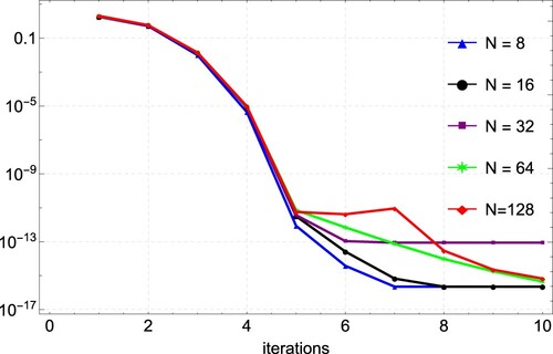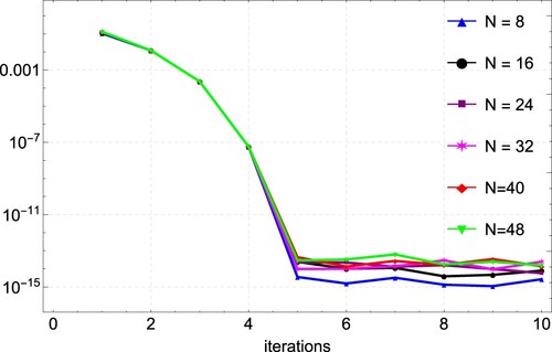Our results are also better compared to the results of [29] obtained by Green‘s function. The agreement between the exact and numerical solutions is depicted in Figure 1, with the errors from the different values of N again shown in Figure 2. In Figure 3, we present the convergence plots of the quasilinearization technique. The method reaches full convergence after only 6 iterations.

Figure 1. Comparison of the exact and approximate solution plots for Example 6.1, showing a good agreement between the two.

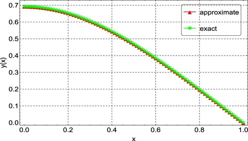
Figure 2. Error plots for the approximation of Example 6.1 for varying values of N.

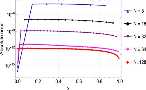
Figure 3. Convergence plots for the approximation of Example 6.1 for varying values of N, showing convergence after 6 iterations.

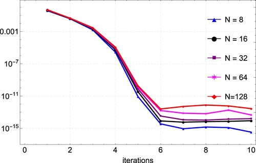
Table 1. Maximum absolute error ($L_{\mathrm{\infty }}$) for Example 6.1.

Present method (CFDM)			Singh et al. [29]		Singh et al. [33]
N	Error norm ($L_{\mathrm{\infty }}$)	ROC	N	Error norm ($L_{\mathrm{\infty }}$)	N	Error norm ($L_{\mathrm{\infty }}$)
8	5.627e−05		4	4.69144e−02	8	7.80e−04
16	1.45823e−07	8.16582	6	6.92128e−03	16	1.94e−04
32	1.37249e−09	6.42723	8	8.25260e−04	32	4.84e−05
64	5.62594e−12	7.75156	10	1.08089e−04	64	1.21e−06
					128	3.02e−06
					256	7.55e−07
					512	1.89e−07
					1024	4.72e−08

Example 6.2

Consider the Lane–Emden equation with Dirichlet-type boundary conditions $y^{\mathrm{\prime }\mathrm{\prime }}\left(x\right)+\frac{0.5}{x}{y}^{\mathrm{\prime }}\left(x\right)+x^2{e}^{y(x)}(14-16x^4{e}^{y(x)})=0,$with boundary conditions: $\begin{array}{rl}& y(0)=\ln \left(\frac{1}{4}\right)\mathrm{and}y(1)=\ln \left(\frac{1}{5}\right),\\ & \mathrm{Exact}\mathrm{solution}:y(x)=\ln \left(\frac{1}{x^4+4}\right).\end{array}$

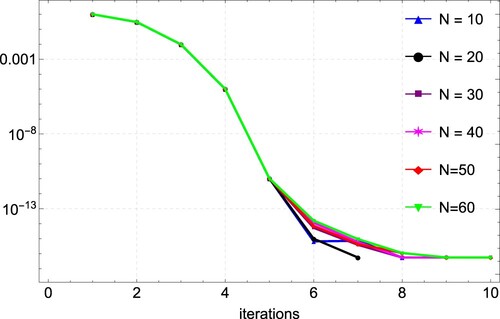
The maximum absolute errors ($L_{\mathrm{\infty }}$) of Example 6.2 are presented in Table 2 along with the results obtained in [33]. Table 2 shows that the proposed method gives accurate results with fewer grid points compared to the results in [33]. Figure 4 depicts the solution of Example 6.2. The errors are also shown in Figure 5 for the different values of N. Figure 6 shows that 5 iterations of the quasilinearization are required to reach full convergence.

Table 2. Maximum absolute error ($L_{\mathrm{\infty }}$) for Example 6.2.

Present method (CFDM)				Singh et al. [33]
N	h	Error norm ($L_{\mathrm{\infty }}$)	Time(s)	N	Error norm ($L_{\mathrm{\infty }}$)
8	0.125	5.17898e−05	0.0081017	8	3.96e−04
16	0.0625	3.97123e−08	0.0103628	16	5.71e−05
32	0.03125	5.65056e−10	0.0245085	32	1.44e−06
64	0.015625	2.79043e−12	0.0813154	64	3.61e−06
			0.279279	128	9.04e−07
				256	2.26e−07
				512	5.65e−08
				1024	1.41e−08

Figure 4. Comparison of the exact and approximate solution plots for Example 6.2, showing a good agreement between the two.

Figure 5. Error plots for the approximation of Example 6.2 for varying values of N.

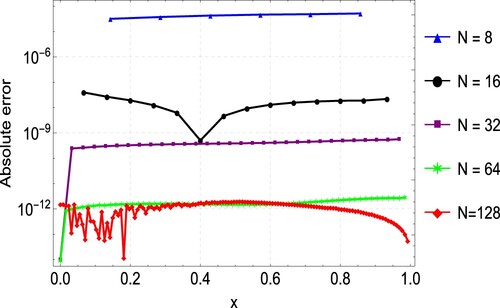
Figure 6. Convergence plots for the approximation of Example 6.2 for varying values of N.

Example 6.3

Consider the Lane–Emden equation with Neumaan-type boundary conditions $y^{\mathrm{\prime }\mathrm{\prime }}\left(x\right)+\frac{2}{x}{y}^{\mathrm{\prime }}(x)+e^{y(x)}(6-4x^2{e}^{y(x)})=0,$with boundary conditions: $\begin{array}{rl}& y^{\mathrm{\prime }}(0)=0\mathrm{and}{y}^{\mathrm{\prime }}(1)=-\frac{2}{5},\\ & \mathrm{Exact}\mathrm{solution}:y(x)=\ln \left(\frac{1}{x^2+4}\right).\end{array}$

The results of Example 6.3 are similar to those of the previous examples. Figure 7 shows the plots of the exact and numerical solution, which are in good agreement. The maximum absolute error and rates of convergence (ROC) are presented in Table 3, with results from Singh et al. [33] included. As shown in the table, the proposed method gives accurate results with fewer grid points compared to the results in [33]. Plots of the maximum absolute errors for various values of N are shown in Figure 8. Finally, Figure 9 shows the convergence plots for the various N values. It can be seen from the plot that the method reaches full convergence after 5 iterations.

Figure 7. Comparison of the exact and approximate solution plots for Example 6.3 showing a good agreement between the two.

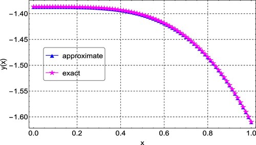
Table 3. Maximum absolute error ($L_{\mathrm{\infty }}$) for Example 6.3.

Present method (CFDM)				Singh et al. [33]
N	h	Error norm ($L_{\mathrm{\infty }}$)	ROC	N	Error norm ($L_{\mathrm{\infty }}$)
10	0.125	2.8657e−06		8	1.95e−03
20	0.05	2.16368e−08	6.53918	16	4.89e−04
40	0.025	1.30177e−10	7.11041	32	1.22e−04
80	0.0125	4.01679e−13	8.1897	64	3.06e−05
				128	7.65e−06
				256	1.91e−06
				512	4.78e−07
				1024	1.20e−07

Figure 8. Error plots for the approximation of Example 6.3 for varying values of N.

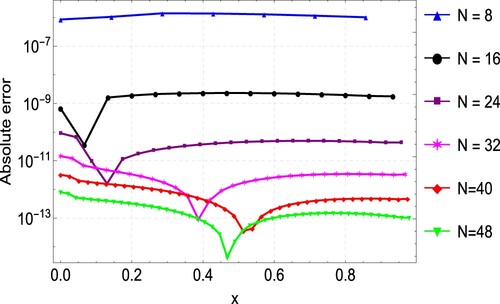
Figure 9. Convergence plots for the approximation of Example 6.3 for varying values of N showing convergence after 5 iterations.

Example 6.4

Consider the Lane–Emden equation describing the equilibrium of the isothermal gas sphere $y^{\mathrm{\prime }\mathrm{\prime }}(x)+\frac{2}{x}{y}^{\mathrm{\prime }}(x)+y^5(x)=0,$with boundary conditions: $\begin{array}{rl}& y^{\mathrm{\prime }}(0)=0\mathrm{and}y(1)=\sqrt{\frac{3}{4}},\\ & \mathrm{Exact}\mathrm{solution}:y=\sqrt{\frac{3}{3+3x^2}}.\end{array}$

For Example 6.4, we also compute the approximate solution using the proposed CFDM for various values of N. Likewise, the error norm and rates of convergence are presented in Table 4. Table 4 presents the comparison of results obtained by CFDM, Taylor wavelet method [60], variation iteration method [17], and finite difference method [21]. It can be seen from the table that CFDM produces better results. A graphical comparison of the CFDM results and the exact solution is shown in Figure 10. Plots of the absolute errors for various N values is shown in Figure 11. Lastly, Figure 12 shows the convergence plots for the various N values. The plot indicates the method reaches full convergences after 5 iterations.

Figure 10. Comparison of the exact and approximate solution plots for Example 6.4, showing a good agreement between the two.

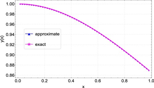
Figure 11. Error plots for the approximation of Example 6.4 for varying values of N.

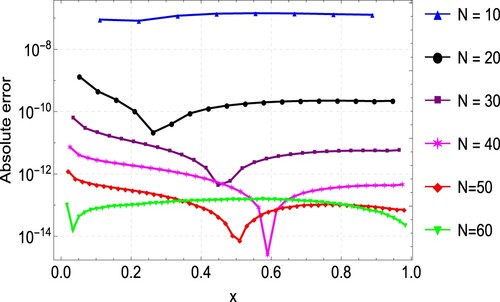
Figure 12. Convergence plots for the approximation of Example 6.4 for varying values of N, showing convergence after 5 iterations.

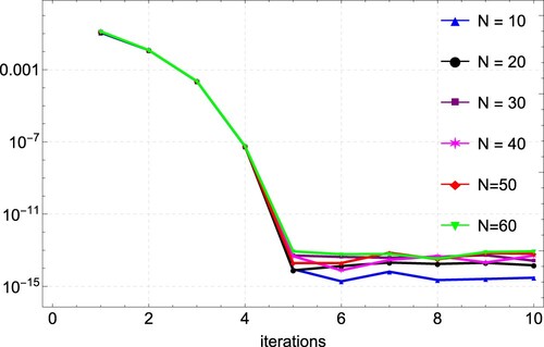
Table 4. Maximum absolute error ($L_{\mathrm{\infty }}$) and $\text{ROC}$ for Example 6.4.

Present method (CFDM)			Gümgüm [60]	Kanth et al. [17]	Chawla et al. [21]
N	Error norm ($L_{\mathrm{\infty }}$)	ROC	Error norm ($L_{\mathrm{\infty }}$)	Error norm ($L_{\mathrm{\infty }}$)	N	Error norm ($L_{\mathrm{\infty }}$)
10	2.79012e−07		3.24e−06	3.92e−04	16	3.64e−04
20	6.79228e−09	5.91062			32	2.49e−05
30	3.39322e−10	7.01049			64	1.6e−06
40	3.87994e−11	7.26498			128	1.01e−07
50	7.28173e−12	7.28756

Example 6.5

Consider the Lane–Emden equation with boundary conditions that arise in a thermal explosion in a cylindrical vessel. $y^{\mathrm{\prime }\mathrm{\prime }}(x)+\frac{1}{x}{y}^{\mathrm{\prime }}(x)+e^{y(x)}=0,$with boundary conditions: $\begin{array}{rl}& y^{\mathrm{\prime }}(0)=0\mathrm{and}y(1)=0,\\ & \mathrm{Exact}\mathrm{solution}:y=2\ln \left(\frac{4-2\sqrt{2}}{(3-2\sqrt{2})x^2+1}\right).\end{array}$

As we did before, in Example 6.5, we also compute the approximate solution using the proposed CFDM for various values of N. Likewise, the error norms and convergence rates are presented in Table 5. Table 5 presents the comparison of results obtained by CFDM, quartic trigonometric B-spline collocation method [27] and finite difference method [21]. It can be seen from the table that CFDM produces better results. A graphical comparison of the CFDM results and the exact solution is shown in Figure 13. Plots of the absolute errors for various N values is shown in Figure 14. Lastly, Figure 15 shows the convergence plots for the various N values. The plot indicates the method reaches full convergences after 6 iterations.

Table 5. Maximum absolute error ($L_{\mathrm{\infty }}$) and $\text{ROC}$ for Example 6.5.

Present method (CFDM)			Chawla et al. [21]		Alam et al. [27]
N	Error norm ($L_{\mathrm{\infty }}$)	ROC	N	Error norm ($L_{\mathrm{\infty }}$)	N	Error norm ($L_{\mathrm{\infty }}$)
10	1.62155e−07		16	2.52e−03	16	1.34663e−08
20	8.15177e−10	7.08351	32	1.83e−04	32	7.86881e−10
30	3.50054e−11	7.44437	64	1.28e−05	64	4.7697e−11
40	3.81284e−12	7.48358	128	8.33e−07	128	2.94776e−12
50	6.66689e−13	7.6396			256	1.67977e−13

Figure 13. Comparison of the exact and approximate solution plots for Example 6.5, showing good agreement between the two.

Figure 14. Error plots for the approximation of Example 6.5 for varying values of N.

Figure 15. Convergence plots for the approximation of Example 6.5 for varying values of N, showing convergence after 6 iterations.

Example 6.6

Consider the Lane–Emden equation with Neumann-Robin type boundary conditions $y^{\mathrm{\prime }\mathrm{\prime }}\left(x\right)+\frac{2}{x}{y}^{\mathrm{\prime }}\left(x\right)+e^{-y(x)}=0,$subject to $y^{\mathrm{\prime }}(0)=0\mathrm{and}2y(1)+y^{\mathrm{\prime }}(1)=0.$

The analytic solution of Example 6.6 is unknown. We have solved the above example using the proposed CFDM for different values of N. Table 6 presents the approximate solutions and compared with the solution acquired by B-spline collocation [27] and Haar wavelet collocation method [33,61]. Table 6 shows that our results agree with results in [27,33,61]. Figure 16 shows the approximate solution of Example 6.6.

Figure 16. Approximate solution plots for Example 6.6 for N = 20.

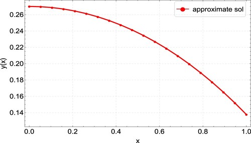
Table 6. Maximum absolute error ($L_{\mathrm{\infty }}$) for Example 6.6.

Present method (CFDM)
x	N = 10	N = 20	Alam et al. [27]	Singh et al. [61]	Singh et al. [33]
0.1	0.268756901799	0.268756900638	0.2697159	0.26349926	0.268755437
0.2	0.264932818575	0.264932817546	0.2687104	0.25965525	0.264931354
0.3	.2585397904233	0.258539789390	0.2649118	0.25322880	0.258538326
0.4	0.249548181308	0.249548180263	0.2585270	0.24418997	0.249546718
0.5	0.237915888665	0.237915887598	0.2495394	0.23249622	0.237914425
0.6	0.223587708284	0.223587707191	0.2440578	0.21809176	0.223586244
0.7	0.206494484164	0.206494483034	0.2310872	0.20090669	0.206493019
0.8	0.186552015349	0.186552014177	0.2153874	0.18085589	0.186550548
0.9	0.163659682834	0.163659681592	0.1968819	0.15783764	0.163658211
1.0	0.137698747815	0.137698746625	0.1754788	0.13173190	0.137697271

Example 6.7

Consider the Lane–Emden equation with Dirichlet-type boundary conditions $y^{\mathrm{\prime }\mathrm{\prime }}\left(x\right)+\frac{2}{x}{y}^{\mathrm{\prime }}\left(x\right)+-\frac{ny(x)}{y(x)+k}=00\le x\le 1$subject to $y^{\mathrm{\prime }}(0)=ln(2)\mathrm{and}5y(1)+y^{\mathrm{\prime }}(1)=5$

Like the previous example, the analytic solution of Example 6.7 is unknown. We have solved the above example using the proposed CFDM for different values of N. Table 7 presents the approximate solutions with comparisons with solutions acquired by Taylor wavelet method [60] and Haar wavelet collocation method [33]. Table 7 shows that our results agree with results in [33,60]. Figure 17 shows the approximate solution of Example 6.7.

Figure 17. Approximate solution plots for Example 6.7 for N = 20.

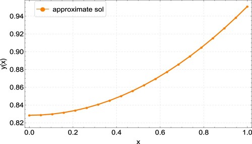
Table 7. Maximum absolute error ($L_{\mathrm{\infty }}$) for Example 6.7.

Present method (CFDM)
x	N = 10	N = 20	Gümgüm [60]	Singh [33]
0.1	0.829706092436	0.829706092434	0.8297063594	0.829706118
0.2	0.833374733596	0.833374733591	0.8333750006	0.833374759
0.3	0.839489913959	0.839489913954	0.8394901811	0.839489939
0.4	0.848052785001	0.848052784996	0.8480530523	0.848052810
0.5	0.859064927173	0.859064927169	0.8590651943	0.859064951
0.6	0.872528319962	0.872528319958	0.8725285872	0.872528343
0.7	0.888445305626	0.888445305623	0.8884455738	0.888445328
0.8	0.906818548069	0.906818548067	0.9068188164	0.906818569
0.9	0.927650988367	0.927650988366	0.9276512446	0.927651008
1.0	0.950945798498	0.950945798497	0.9509459977	0.950945816

7. Conclusion

In this paper, we presented a highly accurate compact finite difference method (CFDM) to solve Lane–Emden equations with various types of boundary conditions. Convergence of the CFDM was established by using properties of the standard matrix norm. By computing the absolute error norm and rates of convergence, the high accuracy of CFDM is confirmed by comparing its numerical results against the numerical results of the Haar wavelet collation method [33,61] and Adomian decomposition method and Green‘s function [29], Taylor wavelet method [60], variation iteration method [17], finite difference method [21] and B-spline collocation method [27]. We also observe that the CFDM approximate solution is in excellent agreement with the exact solution in all of the considered examples. Numerical results further confirm that the rate of convergence of the presented CFDM is seven, consistent with the theoretical approximation.

Disclosure statement

The authors declare that they have no conflict of interest.

References

- Chandrasekhar S. An introduction to study of stellar structure. New York: Dover; 1967.
- Lima PM, Morgado L. Numerical modeling of oxygen diffusion in cells with Michaelis–Menten uptake kinetics. J Math Chem. 2010;48(1):145–158.
- Dz̆urina J, Grace SR, Jadlovská I, et al. Oscillation criteria for second-order Emden–Fowler delay differential equations with a sublinear neutral term. Math Nachr. 2020;293:910–922.
- Li T, Rogovchenko YV. Oscillation of second-order neutral differential equations. Math Nachr. 2015;288(10):1150–1162.
- Li T, Rogovchenko YV. Oscillation criteria for second-order superlinear Emden–Fowler neutral differential equations. Monatsh Math. 2017;184:489–500.
- Li T, Rogovchenko YV. On asymptotic behavior of solutions to higher-order sublinear Emden–Fowler delay differential equations. Appl Math Lett. 2017;67:53–59.
- Frassu S, Li T, Viglialoro G. Improvements and generalizations of results concerning attraction-repulsion chemotaxis models. Math Methods Appl Sci.. 2022;45(17):11067–11078. doi:10.1002/mma.843711078.
- Frassu S, Viglialoro G. Boundedness criteria for a class of indirect (and direct) chemotaxis-consumption models in high dimensions. Appl Math Lett. 2022;132:108108.
- Lane JH. ARR.X–On the law of electric conduction in metals. Am J Sci Arts (1820–1879). 1846;1(2):230.
- Hosseini SG, Abbasbandy S. Solution of Lane–Emden type equations by combination of the spectral method and Adomian decomposition method. Math Probl Eng. 2015;2015:1–10. doi:10.1155/2015/534754.
- Liao S. A new analytic algorithm of Lane–Emden type equations. Appl Math Comput. 2003;142(1):1–16. doi:10.1016/S0096-3003(02)00943-8.
- Wazwaz AM. A new algorithm for solving differential equations of Lane–Emden type. Appl Math Comput. 2001;118(2–3):287–310. doi:10.1016/S0096-3003(99)00223-4.
- Mittal RC, Nigam R. Solution of a class of singular boundary value problems. Numer Algorithms. 2008;47(2):169–179.
- Ghorbani A, Bakherad M. A variational iteration method for solving nonlinear Lane–Emden problems. New Astron. 2017;54:1–6. doi:10.1016/j.newast.2016.12.004.
- Wazwaz AM, Rach R. Comparison of the Adomian decomposition method and the variational iteration method for solving the Lane–Emden equations of the first and second kinds. Kybernetes. 2011;40(9/10):1305–1318.
- Wazwaz AM. Variational iteration method for solving nonlinear singular boundary value problems arising in various physical models. Commun Nonlinear Sci Numer Simul. 2011;16(10):3881–3886. doi:10.1016/j.cnsns.2011.02.026.
- Kanth AR, Aruna K. He's variational iteration method for treating nonlinear singular boundary value problems. Comput Math Appl. 2010;60(3):821–829. doi:10.1016/j.camwa.2010.05.029.
- Sharma P, Gupta VG. Solving singular initial value problems of Emden–Fowler and Lane–Emden type. Int J Appl Math Comput. 2009;1(4):206–212.
- Khan Y, Svoboda Z, Šmarda Z. Solving certain classes of Lane–Emden type equations using the differential transformation method. Adv Differ Equ. 2012;2012(1):1–11.
- Singh OP, Pandey RK, Singh VK. An analytic algorithm of Lane–Emden type equations arising in astrophysics using modified homotopy analysis method. Comput Phys Commun. 2009;180(7):1116–1124. doi:10.1016/j.cpc.2009.01.012.
- Chawla MM, Subramanian R, Sathi HL. A fourth order method for a singular two-point boundary value problem. BIT Numer Math. 1988;28(1):88–97.
- Pandey RK, Singh AK. On the convergence of fourth-order finite difference method for weakly regular singular boundary value problems. Int J Comput Math. 2004;81(2):227–238. doi:10.1080/00207160310001650116.
- Jamet P. On the convergence of finite-difference approximations to one-dimensional singular boundary-value problems. Numer Math. 1970;14(4):355–378.
- Kadalbajoo MK, Kumar V. B-spline method for a class of singular two-point boundary value problems using optimal grid. Appl Math Comput. 2007;188(2):1856–1869. doi:10.1016/j.amc.2006.11.050.
- Çağlar H, Çağlar N, Özer M. B-spline solution of non-linear singular boundary value problems arising in physiology. Chaos Solitons Fract. 2009;39(3):1232–1237. doi:10.1016/j.chaos.2007.06.007.
- Alam MP, Begum T, Khan A. A new spline algorithm for solving non-isothermal reaction diffusion model equations in a spherical catalyst and spherical biocatalyst. Chem Phys Lett. 2020;754:137651. doi:10.1016/j.cplett.2020.137651.
- Alam MP, Begum T, Khan A. A high-order numerical algorithm for solving Lane–Emden equations with various types of boundary conditions. Comput Appl Math. 2021;40(6):1–28. doi:10.1007/s40314-021-01591-7.
- Singh R, Das N, Kumar J. The optimal modified variational iteration method for the Lane–Emden equations with Neumann and Robin boundary conditions. Eur Phys J Plus. 2017;132(6):1–11. doi:10.1140/epjp/i2017-11521-x.
- Singh R, Kumar J, Nelakanti G. Numerical solution of singular boundary value problems using Green's function and improved decomposition method. J Appl Math Comput. 2013;43:409–425. doi:10.1007/s12190-013-0670-4.
- Singh R, Kumar J. An efficient numerical technique for the solution of nonlinear singular boundary value problems. Comput Phys Commun. 2014;185(4):1282–1289. doi:10.1016/j.cpc.2014.01.002.
- Kanth AR, Reddy YN. A numerical method for singular two point boundary value problems via Chebyshev economizition. Appl Math Comput. 2003;146(2–3):691–700. doi:10.1016/S0096-3003(02)00613-6.
- Danish M, Kumar S, Kumar S. A note on the solution of singular boundary value problems arising in engineering and applied sciences: use of OHAM. Comput Chem Eng. 2012;36:57–67. doi:10.1016/j.compchemeng.2011.08.008.
- Singh R, Garg H, Guleria V. Haar wavelet collocation method for Lane–Emden equations with Dirichlet, Neumann and Neumann–Robin boundary conditions. J Comput Appl Math. 2019;346:150–161. doi:10.1016/j.cam.2018.07.004.
- Al-Khaled K. Theory and computation in singular boundary value problems. Chaos Solitons Fract. 2007;33(2):678–684. doi:10.1016/j.chaos.2006.01.047.
- Kanth AR, Aruna K. Solution of singular two-point boundary value problems using differential transformation method. Phys Lett A. 2008;372(26):4671-4673. doi:10.1016/j.physleta.2008.05.019.
- Yildirim A, Agirseven D. The homotopy perturbation method for solving singular initial value problems. Int J Nonlinear Sci Numer Simul. 2009;10(2):235–238. doi:10.1515/IJNSNS.2009.10.2.235.
- Iqbal S, Javed A. Application of optimal homotopy asymptotic method for the analytic solution of singular Lane–Emden type equation. Appl Math Comput. 2011;217(19):7753–7761. doi:10.1016/j.amc.2011.02.083.
- Isik OR, Sezer M. Bernstein series solution of a class of Lane–Emden type equations. Math Probl Eng. 2013;2013:1–9. doi:10.1155/2013/423797.
- Lele SK. Compact finite difference schemes with spectral-like resolution. J Comput Phys. 1992;103(1):16–42.
- Gupta MM, Kouatchou J, Zhang J. Comparison of second-and fourth-order discretizations for multigrid Poisson solvers. J Comput Phys. 1997;132(2):226–232.
- Sari M, Gürarslan G. A sixth-order compact finite difference scheme to the numerical solutions of Burgers’ equation. Appl Math Comput. 2009;208(2):475–483.
- Liao W. An implicit fourth-order compact finite difference scheme for one-dimensional Burgers’ equation. Appl Math Comput. 2008;206(2):755–764.
- Zhao J, Davison M, Corless RM. Compact finite difference method for American option pricing. J Comput Appl Math. 2007;206(1):306–321. doi:10.1016/j.cam.2006.07.006.
- Shah A, Yuan L, Khan A. Upwind compact finite difference scheme for time-accurate solution of the incompressible Navier–Stokes equations. Appl Math Comput. 2010;214(9):320–3213.
- Zhao J, Corless RM. Compact finite difference method for integro-differential equations. Appl Math Comput. 2006;177(1):271–288. doi:10.1016/j.amc.2005.11.007.
- Zhao J. Compact finite difference methods for high order integro-differential equations. Appl Math Comput. 2013;221:66–78. doi:10.1016/j.amc.2013.06.030.
- Li J, Visbal MR. High-order compact schemes for nonlinear dispersive waves. J Sci Comput. 2006;26(1):1–23.
- Düring B, Fournié M, Jüngel A. High order compact finite difference schemes for a nonlinear Black–Scholes equation. Int J Theor Appl Finance. 2003;6(07):767–789.
- Fournie M. High order compact finite difference schemes for a nonlinear Black–Scholes equation. University of Konstanz Center of Finance and Econometrics Discussion Paper (01/07); 2001.
- Mathale D, Dlamini PG, Khumalo M. Compact finite difference relaxation method for chaotic and hyperchaotic initial value systems. Comput Appl Math. 2018;37(4):5187–5202.
- Kouagou JN, Dlamini PG, Simelane SM. On the multi-domain compact finite difference relaxation method for high dimensional chaos: the nine-dimensional Lorenz system. Alex Eng J. 2020;59(4):2617–2625. doi:10.1016/J.AEJ.2020.04.025.
- Dlamini PG, Khumalo M. A new compact finite difference quasilinearization method for nonlinear evolution partial differential equations. Open Math. 2017;15(1):1450–1462.
- Zhao J. Highly accurate compact mixed methods for two point boundary value problems. Appl Math Comput. 2007;188(2):1402–1418. doi:10.1016/j.amc.2006.11.006.
- Zhao J, Zhang T, Corless RM. Convergence of the compact finite difference method for second-order elliptic equations. Appl Math Comput. 2006;182(2):1454–1469. doi:10.1016/j.amc.2006.05.033.
- Pettigrew MF, Rasmussen HA. Compact method for second-order boundary value problems on nonuniform grids. Comput Math Appl. 1996;31(9):1–16. doi:10.1016/0898-1221(96)00037-5.
- Holsapple R, Venkataraman R, Doman D. New, fast numerical method for solving two-point boundary-value problems. J Guid Control Dyn. 2004;27(2):301–304. doi:10.2514/1.1329.
- Bellman RE, Kalaba RE. Quasilinearization and nonlinear boundary-value problems. New York: Elsevier; 1965.
- Mandelzweig VB, Tabakin F. Quasilinearization approach to nonlinear problems in physics with application to nonlinear ODEs. Comput Phys Commun. 2001;141(2):268–281.
- Keller HB. Numerical solution of two point boundary value problems. Philadelphia; Society for Industrial and Applied Mathematics: 1976. (CBMS regional conference series in applied mathematics; vol. 24).
- Gümgüm S. Taylor wavelet solution of linear and nonlinear Lane–Emden equations. Appl Numer Math. 2020;158:44–53. doi:10.1016/j.apnum.2020.07.019.
- Singh R, Shahni J, Garg H, et al. Haar wavelet collocation approach for Lane–Emden equations arising in mathematical physics and astrophysics. Eur Phys J Plus. 2019;134(11):548. doi:10.1140/epjp/i2019-12889-1.