Parameter uniform hybrid numerical method for time-dependent singularly perturbed parabolic differential equations with large delay

ABSTRACT

In this study, to solve the singularly perturbed delay convection–diffusion–reaction problem, we proposed a hybrid numerical scheme that converges uniformly. Parabolic right boundary layer outcomes from the presence of the small perturbation parameter. To grip this layer behaviour, the problem is solved by Bakhvalov–Shishkin mesh for spatial domain discretization and uniform mesh for temporal domain discretization. A hybrid scheme consisting of a non-polynomial spline scheme for fine mesh and a midpoint upwind scheme for coarse mesh is used to discretize the spatial derivative, while an implicit Euler scheme is used to discretize the time derivative. To make computed solutions more accurate and increase rate of convergence of the scheme, we applied Richardson extrapolation technique. The stability and convergence of the scheme are established. The scheme has a second order of convergence in the discrete supreme norm and is parametric uniformly convergent. The scheme's application is demonstrated through two test problems.

KEYWORDS:

• Non-polynomial spline
• Bakhvalov–Shishkin mesh
• hybrid numerical scheme
• parametric convergent
• Richardson extrapolation

MATHEMATICS SUBJECT CLASSIFICATIONS:

• 65N12
• 65N06
• 65N15

1. Introduction

Differential equations that have their highest-order derivatives multiplied by a perturbation parameter ε are said to be singularly perturbed equations. The perturbation parameter takes an arbitrary value in $(0,1]$ which forms interior and/or boundary layers, that is, narrow subdomains on which the solution has a steep gradient. In these subdomains, when ε approaches zero, the derivatives of the solution increase rapidly. Singularly perturbed delay partial differential equations are singularly perturbed problems that involve one or more delay terms. The modelling of many real-world phenomena, including physical, chemical, and biological systems, which are characterized by variables that are both temporal and spatial, uses these equations [1–4]. Particularly, in a better way to comprehend how singularly perturbed delay parabolic differential equations are applied, one can see the example given in [3] , which is being used to model a furnace that processes metal sheet. In the example,the controller's finite speed is the cause of the delay.

Because of the boundary layer's existence in the singularly perturbed problem solution, the classical finite difference methods provide an unsatisfactory numerical result. So various numerical approaches have been developed for solving these problems, which need the so-called uniformly convergent method regardless of the perturbation parameter's value [5,6]. Fitted mesh and fitted operator are the two main numerical methods for constructing a uniformly convergent scheme. Fitted mesh methods use layer-adapted non-uniform mesh, which is dense in the layer(s), while the fitted operator uses an exponentially fitted scheme. There are also other parameter-uniform numerical approximations approaches for singularly perturbed problems, such as domain decomposition [7,8] and grid equidistribution [9]. One can read literature on singularly perturbed delay problems in [10–15]. Richardson extrapolation technique is a numerical method used to improve the accuracy of numerical solutions of differential equations. In the context of singularly perturbed problems, the Richardson extrapolation technique has been used to improve the accuracy of numerical schemes. The reader can get an exposition of this approach in [16–19].

Using spline approximation methods, many authors developed uniformly convergent numerical methods for singularly perturbed delay convection–diffusion–reaction boundary value problems with Dirichlet boundary conditions. To name a few, a second-order exponentially fitted spline and B-spline collocation non-standard method on uniform mesh by a Negero [20,21], a second-order exponentially fitted tension spline on a uniform mesh, a reaction–diffusion version by Megiso et al. [22], and essentially second-order tension spline on shishkin mesh but a reaction-diffusion version by Murali [23]. A singularly perturbed problem with a large delay is one where the delay parameter exceeds the perturbation parameter; otherwise, it is said to be a singularly perturbed problem with small delay [24,25].To the best of our knowledge, the problem under consideration has not been solved using hybrid finite difference, which comprises midpoint upwind and the non-polynomial spline method on the Bakhvalov–Shishkin (B-S) mesh, till date. Motivated by articles [23,26], we developed a uniformly convergent numerical method for solving singularly perturbed parabolic convection–diffusion boundary value problem with a large time delay. The present work has novelties in terms of the existing work. The proposed method is free from convergency spoiled by a logarithmic factor, unlike using the method on Shishkin method. Additionally, the integration of Bakhvalov mesh and the non-polynomial spline method in the layer region potentially provide stability and an accurate numerical solution for singularly perturbed delay parabolic differential equations and allow for more flexibility in choosing the basis function used to approximate the function.

The rest of the paper is structured as follows: In Section 2 continuous problem formulation is described. Section 3 describes bounds on the continuous solution and its derivatives. In Section 4, the numerical scheme is implemented. Section 5 discusses the method's uniform convergence analysis. In Section 6, The technique of Richardson extrapolation has been explained. In Section 7, numerical experiments are illustrated in order to verify the theoretical result. The main conclusions are summarized in the last section.

Throughout the paper, C,$C_1$, and $C_2$, have been taken as generic positive constants that are independent of mesh size, mesh point, and perturbation parameter.

In the following sections $\Vert g\Vert$ denote standard supremum norm and defined as $\Vert g\Vert =\underset{(x,t)\in D}{sup}|g(x,t)|$ defined on domain D.

2. Statement of the problem

The class of singularly perturbed delay parabolic convection–diffusion problems that we examine is as follows. (1) $(\frac{\mathrm{\partial }}{\mathrm{\partial }t}+{\mathcal{L}}_{\epsilon })z(x,t)+c(x,t)z(x,t-\tau )=f(x,t),(x,t)\in D,$(1) with the subsequent interval and boundary conditions: (2) $\begin{array}{rl}z(x,t)& ={\psi }_b(x,t),(x,t)\in {\mathrm{\Gamma }}_b=[0,1]\times [-\tau ,0],\\ z(0,t)& ={\psi }_l(t),(0,t)\in {\mathrm{\Gamma }}_l=\{(0,t),0\le t\le T\},\\ z(1,t)& ={\psi }_r(t),(1,t)\in {\mathrm{\Gamma }}_r=\{(1,t),0\le t\le T\},\end{array}$(2) where, ${\mathcal{L}}_{\epsilon }=-\epsilon \frac{{\mathrm{\partial }}^2}{\mathrm{\partial }{x}^2}+a(x)\frac{\mathrm{\partial }}{\mathrm{\partial }x}+b(x,t).$Here $D=\mathrm{\Omega }\times \mathrm{\Lambda },\mathrm{\Lambda }=(0,T],\mathrm{\Omega }=(0,1)$ and $\mathrm{\Gamma }={\mathrm{\Gamma }}_r\cup {\mathrm{\Gamma }}_b\cup {\mathrm{\Gamma }}_l.$ Also $0<\epsilon \ll 1$ and $\tau >0$ are respectively, perturbation and delay parameters. The functions $f(x,t),c(x,t)$, and $b(x,t)$ in $\overline{D}$, $a(x)$ in $\overline{\mathrm{\Omega }}$, and ${\psi }_l(t),{\psi }_b(x,t),$ and ${\psi }_r(t)$ in Γ are assumed to be sufficiently smooth, bounded and independent of ε, that satisfy $a(x)\ge \alpha >0,c(x,t)\ge \gamma >0,b(x,t)\ge \beta >0,(x,t)\in \overline{D}.$It is assumed that the terminal time T satisfies the condition $T=\mathrm{k\tau }$, where k is positive integer. Under the aforementioned circumstances, the boundary layer of width $\mathcal{O}(\epsilon )$ along x = 1 is displayed in the boundary value problem Equations (1(1) $(\frac{\mathrm{\partial }}{\mathrm{\partial }t}+{\mathcal{L}}_{\epsilon })z(x,t)+c(x,t)z(x,t-\tau )=f(x,t),(x,t)\in D,$(1) )–(2(2) $\begin{array}{rl}z(x,t)& ={\psi }_b(x,t),(x,t)\in {\mathrm{\Gamma }}_b=[0,1]\times [-\tau ,0],\\ z(0,t)& ={\psi }_l(t),(0,t)\in {\mathrm{\Gamma }}_l=\{(0,t),0\le t\le T\},\\ z(1,t)& ={\psi }_r(t),(1,t)\in {\mathrm{\Gamma }}_r=\{(1,t),0\le t\le T\},\end{array}$(2) ) solution. The problem under consideration occurs in fluid dynamics. In this engineering field, the coefficient of the convective term represents the f mass transfer rate [27]. If this transfer rate is influenced by external factors such as temperature gradient or fluid velocity variation, the convective flow is more spatially dependent, i.e. it is time-invariant $a(x)$. However, it is important to note that there are situations where there is both significant temporal and spatial variation occurs, so the coefficient of the convection term is $a(x,t).$ In such cases, the convergence analysis is general and is covered in [28,29].

3. Bounds on the solution and its derivatives

If the data are sufficiently smooth in their domain of definition and meet the following compatibility conditions at the corner points $(0,-\tau )$,$(1,-\tau )$,$(0,0)$, and $(1,0)$, then the existence and uniqueness of the Equations (1(1) $(\frac{\mathrm{\partial }}{\mathrm{\partial }t}+{\mathcal{L}}_{\epsilon })z(x,t)+c(x,t)z(x,t-\tau )=f(x,t),(x,t)\in D,$(1) )–(2(2) $\begin{array}{rl}z(x,t)& ={\psi }_b(x,t),(x,t)\in {\mathrm{\Gamma }}_b=[0,1]\times [-\tau ,0],\\ z(0,t)& ={\psi }_l(t),(0,t)\in {\mathrm{\Gamma }}_l=\{(0,t),0\le t\le T\},\\ z(1,t)& ={\psi }_r(t),(1,t)\in {\mathrm{\Gamma }}_r=\{(1,t),0\le t\le T\},\end{array}$(2) ) solution can be guaranteed. (3) $\begin{array}{rl}& {\psi }_b(0,0)={\psi }_l(0),\\ & {\psi }_b(1,0)={\psi }_r(0),\\ & {\frac{\mathrm{d}{\psi }_l}{\mathrm{d}t}|}_{t=0}-\epsilon {\frac{{\mathrm{\partial }}^2{\psi }_b}{\mathrm{\partial }{x}^2}|}_{(0,0)}+a(0){\frac{\mathrm{\partial }{\psi }_b}{\mathrm{\partial }x}|}_{(0,0)}+b(0,0){\psi }_b(0,0)+c(0,0){\psi }_b(0,-\tau )=f(0,0),\\ & {\frac{\mathrm{d}{\psi }_r}{\mathrm{d}t}|}_{t=0}-\epsilon {\frac{{\mathrm{\partial }}^2{\psi }_b}{\mathrm{\partial }{x}^2}|}_{(1,0)}+a(1){\frac{\mathrm{\partial }{\psi }_b}{\mathrm{\partial }x}|}_{(1,0)}+b(1,0){\psi }_b(1,0)+c(1,0){\psi }_b(1,-\tau )=f(1,0).\end{array}$(3)

Lemma 3.1

Maximum Principle

Assume $\eta (x,t)\in C^{2,1}(\overline{D})$, such that $\eta (x,t)\ge 0$, for all $(x,t)\in \mathrm{\Gamma }$ and $(\frac{\mathrm{\partial }}{\mathrm{\partial }t}+{\mathcal{L}}_{\epsilon })\eta (x,t)\ge 0$ for all $(x,t)\in D.$ Then $\eta (x,t)\ge 0$, for all $(x,t)\in \overline{D}.$

Proof.

Let $(x_{\ast },t_{\ast })\in \overline{D}$ such that $\eta (x_{\ast },t_{\ast })=\underset{(x,t)\in \overline{D}}{min}\eta (x,t)$, assume $\eta (x_{\ast },t_{\ast })<0$, clearly $(x_{\ast },t_{\ast })\notin \mathrm{\Gamma }$ and $(x_{\ast },t_{\ast })\in D.$

From Calculus we have,$\frac{\mathrm{\partial }\eta (x_{\ast },t_{\ast })}{\mathrm{\partial }x}=0=\frac{\mathrm{\partial }\eta (x_{\ast },t_{\ast })}{\mathrm{\partial }t}$ and $\frac{{\mathrm{\partial }}^2\eta (x_{\ast },t_{\ast })}{\mathrm{\partial }{x}^2}\ge 0$ then from Equations (1(1) $(\frac{\mathrm{\partial }}{\mathrm{\partial }t}+{\mathcal{L}}_{\epsilon })z(x,t)+c(x,t)z(x,t-\tau )=f(x,t),(x,t)\in D,$(1) )–(2(2) $\begin{array}{rl}z(x,t)& ={\psi }_b(x,t),(x,t)\in {\mathrm{\Gamma }}_b=[0,1]\times [-\tau ,0],\\ z(0,t)& ={\psi }_l(t),(0,t)\in {\mathrm{\Gamma }}_l=\{(0,t),0\le t\le T\},\\ z(1,t)& ={\psi }_r(t),(1,t)\in {\mathrm{\Gamma }}_r=\{(1,t),0\le t\le T\},\end{array}$(2) ) we have $(\frac{\mathrm{\partial }}{\mathrm{\partial }t}+{\mathcal{L}}_{\epsilon })\eta (x_{\ast },t_{\ast })<0$ which contradicts to $(\frac{\mathrm{\partial }}{\mathrm{\partial }t}+{\mathcal{L}}_{\epsilon })\eta (x,t)\ge 0.$ Hence $\eta (x,t)\ge 0$, for all $(x,t)\in \overline{D}.$

We divide the time interval $[0,T]$ using the delay term τ, such as $[0,\tau ]$, $[\tau ,2\tau ]$ and so forth, based on the available method of steps [30–33]. On the interval $[0,\tau ]$, in (1(1) $(\frac{\mathrm{\partial }}{\mathrm{\partial }t}+{\mathcal{L}}_{\epsilon })z(x,t)+c(x,t)z(x,t-\tau )=f(x,t),(x,t)\in D,$(1) )–(2(2) $\begin{array}{rl}z(x,t)& ={\psi }_b(x,t),(x,t)\in {\mathrm{\Gamma }}_b=[0,1]\times [-\tau ,0],\\ z(0,t)& ={\psi }_l(t),(0,t)\in {\mathrm{\Gamma }}_l=\{(0,t),0\le t\le T\},\\ z(1,t)& ={\psi }_r(t),(1,t)\in {\mathrm{\Gamma }}_r=\{(1,t),0\le t\le T\},\end{array}$(2) ) becomes the expression $f(x,t)-c(x,t)z(x,t-\tau )$ becomes $f(x,t)-c(x,t){\psi }_b(x,t-\tau )$,which is independent of ε in $\mathrm{\Omega }\times [0,\tau ].$ Hence, for $t\in [0,\tau ]$, (1(1) $(\frac{\mathrm{\partial }}{\mathrm{\partial }t}+{\mathcal{L}}_{\epsilon })z(x,t)+c(x,t)z(x,t-\tau )=f(x,t),(x,t)\in D,$(1) )–(2(2) $\begin{array}{rl}z(x,t)& ={\psi }_b(x,t),(x,t)\in {\mathrm{\Gamma }}_b=[0,1]\times [-\tau ,0],\\ z(0,t)& ={\psi }_l(t),(0,t)\in {\mathrm{\Gamma }}_l=\{(0,t),0\le t\le T\},\\ z(1,t)& ={\psi }_r(t),(1,t)\in {\mathrm{\Gamma }}_r=\{(1,t),0\le t\le T\},\end{array}$(2) ) becomes (4) $\{\begin{array}{l}(\frac{\mathrm{\partial }}{\mathrm{\partial }t}+{\mathcal{L}}_{\epsilon })z(x,t)+c(x,t){\psi }_b(x,t-\tau )=f(x,t),(x,t)\in \mathrm{\Omega }\times (0,\tau ],\\ z(x,0)={\psi }_b(x,0),x\in [0,1],\\ z(0,t)={\psi }_l(t),z(1,t)={\psi }_r(t)t\in (0,\tau ].\end{array}$(4) Now, we decompose the solution $z(x,t)$ in to its singular $w(x,t)$ and regular $v(x,t)$ components as $z(x,t)=v(x,t)+w(x,t).$ The two terms asymptotic expansion for $v(x,t)$ is $v(x,t)=v_0(x,t)+\epsilon v_1(x,t)$, where $v_0(x,t)$ satisfies (5) $\{\begin{array}{l}\frac{\mathrm{\partial }{v}_0(x,t)}{\mathrm{\partial }t}+a(x)\frac{\mathrm{\partial }{v}_0(x,t)}{\mathrm{\partial }x}+b(x,t)v_0(x,t)+c(x,t){\psi }_b(x,t-\tau )=f(x,t),(x,t)\in \mathrm{\Omega }\times (0,\tau ],\\ z(x,0)={\psi }_b(x,0),x\in [0,1],\end{array}$(5) and $v_1(x,t)$ satisfies (6) $\{\begin{array}{l}(\frac{\mathrm{\partial }}{\mathrm{\partial }t}+{\mathcal{L}}_{\epsilon })v_1(x,t)=\frac{{\mathrm{\partial }}^2{v}_0(x,t)}{\mathrm{\partial }{x}^2},(x,t)\in \mathrm{\Omega }\times (0,\tau ],\\ v_1(x,0)=0,x\in [0,1],\\ v_1(0,t)=0,v_1(1,t)=0t\in (0,\tau ].\end{array}$(6) Thus, the regular component $v(x,t)$ satisfies (7) $\{\begin{array}{l}(\frac{\mathrm{\partial }}{\mathrm{\partial }t}+{\mathcal{L}}_{\epsilon })v(x,t)+c(x,t){\psi }_b(x,t-\tau )=f(x,t),(x,t)\in \mathrm{\Omega }\times (0,\tau ],\\ v(x,0)={\psi }_b(x,0),x\in [0,1],\\ v(0,t)=v_0(0,t),v(1,t)=v_0(1,t),t\in (0,\tau ].\end{array}$(7) The singular component $w(x,t)$ satisfy the homogeneous problem: (8) $\{\begin{array}{l}(\frac{\mathrm{\partial }}{\mathrm{\partial }t}+{\mathcal{L}}_{\epsilon })w(x,t)=0,(x,t)\in \mathrm{\Omega }\times (0,\tau ],\\ w(x,0)=0,x\in [0,1],\\ w(0,t)={\psi }_l(t)-v_0(0,t),t\in (0,\tau ],\\ w(1,t)={\psi }_r(t)-v_0(1,t),t\in (0,\tau ].\end{array}$(8) Now, for $t\in [\tau ,2\tau ]$, (1(1) $(\frac{\mathrm{\partial }}{\mathrm{\partial }t}+{\mathcal{L}}_{\epsilon })z(x,t)+c(x,t)z(x,t-\tau )=f(x,t),(x,t)\in D,$(1) )–(2(2) $\begin{array}{rl}z(x,t)& ={\psi }_b(x,t),(x,t)\in {\mathrm{\Gamma }}_b=[0,1]\times [-\tau ,0],\\ z(0,t)& ={\psi }_l(t),(0,t)\in {\mathrm{\Gamma }}_l=\{(0,t),0\le t\le T\},\\ z(1,t)& ={\psi }_r(t),(1,t)\in {\mathrm{\Gamma }}_r=\{(1,t),0\le t\le T\},\end{array}$(2) ) becomes (9) $\{\begin{array}{l}(\frac{\mathrm{\partial }}{\mathrm{\partial }t}+{\mathcal{L}}_{\epsilon })z(x,t)+c(x,t)c(x,t-\tau )=f(x,t),(x,t)\in \mathrm{\Omega }\times (\tau ,2\tau ],\\ z(x,t)=z(x,t),(x,t)\in [0,1]\times [0,\tau ],\\ z(0,t)={\psi }_l(t),z(1,t)={\psi }_r(t)t\in (\tau ,2\tau ].\end{array}$(9) Again, we decompose the solution $z(x,t)$ in to its singular $w(x,t)$ and regular $v(x,t)$ components as $z(x,t)=v(x,t)+w(x,t).$ The two terms asymptotic expansion for $v(x,t)$ is $v(x,t)=v_0(x,t)+\epsilon v_1(x,t)$, where $v_0(x,t)$ satisfies the reduced problem (10) $\{\begin{array}{l}\frac{\mathrm{\partial }{v}_0(x,t)}{\mathrm{\partial }t}+a(x)\frac{\mathrm{\partial }{v}_0(x,t)}{\mathrm{\partial }x}+b(x,t)v_0(x,t)\\ +c(x,t)v_0(x,t-\tau )=f(x,t),(x,t)\in \mathrm{\Omega }\times (\tau ,2\tau ],\\ v_0(x,t)=z(x,t),(x,t)\in [0,1]\times [0,\tau ],\end{array}$(10) and $v_1(x,t)$ satisfies (11) $\{\begin{array}{l}(\frac{\mathrm{\partial }}{\mathrm{\partial }t}+{\mathcal{L}}_{\epsilon })v_1(x,t)+c(x,t)v_1(x,t-\tau )=\frac{{\mathrm{\partial }}^2{v}_0(x,t)}{\mathrm{\partial }{x}^2},(x,t)\in \mathrm{\Omega }\times (\tau ,2\tau ],\\ v_1(x,t)=0,(x,t)\in [0,1]\times [0,\tau ],\\ v_1(0,t)=0=v_1(1,t),t\in (\tau ,2\tau ].\end{array}$(11) Clearly the regular component $v(x,t)$ satisfies the following problem (12) $\{\begin{array}{l}(\frac{\mathrm{\partial }}{\mathrm{\partial }t}+{\mathcal{L}}_{\epsilon })v(x,t)+c(x,t)v(x,t-\tau )=f(x,t),(x,t)\in \mathrm{\Omega }\times (\tau ,2\tau ],\\ v(x,t)=z(x,t),(x,t)\in [0,1]\times [0,\tau ],\\ v(0,t)=v_0(0,t),v(1,t)=v_0(1,t),t\in (\tau ,2\tau ].\end{array}$(12) The singular component $w(x,t)$ satisfy the homogeneous problem: (13) $\{\begin{array}{l}(\frac{\mathrm{\partial }}{\mathrm{\partial }t}+{\mathcal{L}}_{\epsilon })w(x,t)+c(x,t)w(x,t-\tau )=0,(x,t)\in \mathrm{\Omega }\times (\tau ,2\tau ],\\ w(x,t)=0,(x,t)\in [0,1]\times [0,\tau ],\\ w(0,t)={\psi }_l(t)-v_0(0,t),t\in (\tau ,2\tau ],\\ w(1,t)={\psi }_r(t)-v_0(1,t),t\in (\tau ,2\tau ].\end{array}$(13) In the same way, to get the decomposition on $[0,T]$, we extend the decomposition approaches at every partition. This method of steps yields the existence and uniqueness results for all $(x,t)\in \overline{D}$. For the interval $[0,\tau ]$, $z(x,t-\tau )$ is known function,i.e. $f(x,t)-c(x,t){\psi }_b(x,t-\tau )$ is independent of ε, and thus (1(1) $(\frac{\mathrm{\partial }}{\mathrm{\partial }t}+{\mathcal{L}}_{\epsilon })z(x,t)+c(x,t)z(x,t-\tau )=f(x,t),(x,t)\in D,$(1) )–(2(2) $\begin{array}{rl}z(x,t)& ={\psi }_b(x,t),(x,t)\in {\mathrm{\Gamma }}_b=[0,1]\times [-\tau ,0],\\ z(0,t)& ={\psi }_l(t),(0,t)\in {\mathrm{\Gamma }}_l=\{(0,t),0\le t\le T\},\\ z(1,t)& ={\psi }_r(t),(1,t)\in {\mathrm{\Gamma }}_r=\{(1,t),0\le t\le T\},\end{array}$(2) ) becomes a classical singularly perturbed parabolic problem, which can be solved the existing theories [34,35]. In addition, for $[\tau ,2\tau ]$ the existence and uniqueness of a solution of (1(1) $(\frac{\mathrm{\partial }}{\mathrm{\partial }t}+{\mathcal{L}}_{\epsilon })z(x,t)+c(x,t)z(x,t-\tau )=f(x,t),(x,t)\in D,$(1) )–(2(2) $\begin{array}{rl}z(x,t)& ={\psi }_b(x,t),(x,t)\in {\mathrm{\Gamma }}_b=[0,1]\times [-\tau ,0],\\ z(0,t)& ={\psi }_l(t),(0,t)\in {\mathrm{\Gamma }}_l=\{(0,t),0\le t\le T\},\\ z(1,t)& ={\psi }_r(t),(1,t)\in {\mathrm{\Gamma }}_r=\{(1,t),0\le t\le T\},\end{array}$(2) ) is considered in [30,36–38].

Lemma 3.2

[39],Lemma 3.2.

The solution $z(x,t)$ of Equations (1(1) $(\frac{\mathrm{\partial }}{\mathrm{\partial }t}+{\mathcal{L}}_{\epsilon })z(x,t)+c(x,t)z(x,t-\tau )=f(x,t),(x,t)\in D,$(1) )–(2(2) $\begin{array}{rl}z(x,t)& ={\psi }_b(x,t),(x,t)\in {\mathrm{\Gamma }}_b=[0,1]\times [-\tau ,0],\\ z(0,t)& ={\psi }_l(t),(0,t)\in {\mathrm{\Gamma }}_l=\{(0,t),0\le t\le T\},\\ z(1,t)& ={\psi }_r(t),(1,t)\in {\mathrm{\Gamma }}_r=\{(1,t),0\le t\le T\},\end{array}$(2) ) satisfies the following bound:

$|z(x,t)-{\psi }_b(x,0)|\le \mathrm{Ct},(x,t)\in \overline{D},$ where C is independent of ε.

Lemma 3.3

The solution $z(x,t)$ of Equations (1(1) $(\frac{\mathrm{\partial }}{\mathrm{\partial }t}+{\mathcal{L}}_{\epsilon })z(x,t)+c(x,t)z(x,t-\tau )=f(x,t),(x,t)\in D,$(1) )–(2(2) $\begin{array}{rl}z(x,t)& ={\psi }_b(x,t),(x,t)\in {\mathrm{\Gamma }}_b=[0,1]\times [-\tau ,0],\\ z(0,t)& ={\psi }_l(t),(0,t)\in {\mathrm{\Gamma }}_l=\{(0,t),0\le t\le T\},\\ z(1,t)& ={\psi }_r(t),(1,t)\in {\mathrm{\Gamma }}_r=\{(1,t),0\le t\le T\},\end{array}$(2) ) satisfies the following estimate: $|z(x,t)|\le C$,for $(x,t)\in \overline{D}.$

Proof.

Since $t\in [0,T]$ and from Lemma 3.2 we have $|z(x,t)|\le \mathrm{Ct}$, it follows that $|z(x,t)|\le C.$

Lemma 3.4

Uniform Stability Estimate

The ε-uniform bound on the solution $z(x,t)$ of continuous problem equations (1(1) $(\frac{\mathrm{\partial }}{\mathrm{\partial }t}+{\mathcal{L}}_{\epsilon })z(x,t)+c(x,t)z(x,t-\tau )=f(x,t),(x,t)\in D,$(1) )–(2(2) $\begin{array}{rl}z(x,t)& ={\psi }_b(x,t),(x,t)\in {\mathrm{\Gamma }}_b=[0,1]\times [-\tau ,0],\\ z(0,t)& ={\psi }_l(t),(0,t)\in {\mathrm{\Gamma }}_l=\{(0,t),0\le t\le T\},\\ z(1,t)& ={\psi }_r(t),(1,t)\in {\mathrm{\Gamma }}_r=\{(1,t),0\le t\le T\},\end{array}$(2) ) satisfies $|z(x,t)|\le \frac{1}{\beta }\Vert (\frac{\mathrm{\partial }}{\mathrm{\partial }t}+{\mathcal{L}}_{\epsilon })z(x,t)\Vert +max\{|{\psi }_l(t)|,|{\psi }_r(t)|,|{\psi }_b(x,t)|\}.$

Proof.

For the barrier functions $\begin{array}{rl}{\mathrm{\Xi }}^{\pm }(x,t)& =\frac{1}{\beta }\Vert (\frac{\mathrm{\partial }}{\mathrm{\partial }t}+{\mathcal{L}}_{\epsilon })z(x,t)\Vert +max\{|{\psi }_l(t)|,|{\psi }_r(t)|,|{\psi }_b(x,t)|\}\pm z(x,t),\\ & (x,t)\in \overline{D},\end{array}$we have,on ${\mathrm{\Gamma }}_l$ $\begin{array}{rl}{\mathrm{\Xi }}^{\pm }(0,t)& =\frac{1}{\beta }\Vert (\frac{\mathrm{\partial }}{\mathrm{\partial }t}+{\mathcal{L}}_{\epsilon })z(x,t)\Vert +max\{|{\psi }_l(t)|,|{\psi }_r(t)|,|{\psi }_b(x,t)|\}\pm z(0,t)\\ & \ge max\{|{\psi }_l(t)|,|{\psi }_r(t)|,|{\psi }_b(x,t)|\}\pm z(0,t)\\ & \ge 0,\end{array}$on ${\mathrm{\Gamma }}_r$ $\begin{array}{rl}{\mathrm{\Xi }}^{\pm }(1,t)& =\frac{1}{\beta }\Vert (\frac{\mathrm{\partial }}{\mathrm{\partial }t}+{\mathcal{L}}_{\epsilon })z(x,t)\Vert +max\{|{\psi }_l(t)|,|{\psi }_r(t)|,|{\psi }_b(x,t)|\}\pm z(1,t)\\ & \ge max\{|{\psi }_l(t)|,|{\psi }_r(t)|,|{\psi }_b(x,t)|\}\pm z(1,t)\\ & \ge 0,\end{array}$on ${\mathrm{\Gamma }}_b$ $\begin{array}{rl}{\mathrm{\Xi }}^{\pm }(x,t)& =\frac{1}{\beta }\Vert (\frac{\mathrm{\partial }}{\mathrm{\partial }t}+{\mathcal{L}}_{\epsilon })z(x,t)\Vert +max\{|{\psi }_l(t)|,|{\psi }_r(t)|,|{\psi }_b(x,t)|\}\pm z(x,t)\\ & \ge max\{|{\psi }_l(t)|,|{\psi }_r(t)|,|{\psi }_b(x,t)|\}\pm z(x,t)\\ & \ge 0.\end{array}$Furthermore, for all $(x,t)\in D$, $\begin{array}{rl}& (\frac{\mathrm{\partial }}{\mathrm{\partial }t}+{\mathcal{L}}_{\epsilon }){\mathrm{\Xi }}^{\pm }(x,t)\\ & =b(x,t)(\frac{1}{\beta }\Vert (\frac{\mathrm{\partial }}{\mathrm{\partial }t}+{\mathcal{L}}_{\epsilon })z(x,t)\Vert +max\{|{\psi }_l(t)|,|{\psi }_r(t)|,|{\psi }_b(x,t)|\})\\ & \pm (\frac{\mathrm{\partial }}{\mathrm{\partial }t}+{\mathcal{L}}_{\epsilon })z(x,t)\\ & \ge \Vert (\frac{\mathrm{\partial }}{\mathrm{\partial }t}+{\mathcal{L}}_{\epsilon })z(x,t)\Vert +b(x,t)max\{|{\psi }_l(t)|,|{\psi }_r(t)|,|{\psi }_b(x,t)|\}\\ & \pm (\frac{\mathrm{\partial }}{\mathrm{\partial }t}+{\mathcal{L}}_{\epsilon })z(x,t)\\ & \ge \Vert (\frac{\mathrm{\partial }}{\mathrm{\partial }t}+{\mathcal{L}}_{\epsilon })z(x,t)\Vert \pm (\frac{\mathrm{\partial }}{\mathrm{\partial }t}+{\mathcal{L}}_{\epsilon })z(x,t)\\ & \ge 0.\end{array}$Therefore, by using maximum principle stated in Lemma 3.1, we obtain ${\mathrm{\Xi }}^{\pm }(x,t)\ge 0.$ for all $(x,t)\in \overline{D}$. Accordingly, we get the required bound.

Theorem 3.1

The derivatives of exact solution $z(x,t)$ of Equations (1(1) $(\frac{\mathrm{\partial }}{\mathrm{\partial }t}+{\mathcal{L}}_{\epsilon })z(x,t)+c(x,t)z(x,t-\tau )=f(x,t),(x,t)\in D,$(1) )–(2(2) $\begin{array}{rl}z(x,t)& ={\psi }_b(x,t),(x,t)\in {\mathrm{\Gamma }}_b=[0,1]\times [-\tau ,0],\\ z(0,t)& ={\psi }_l(t),(0,t)\in {\mathrm{\Gamma }}_l=\{(0,t),0\le t\le T\},\\ z(1,t)& ={\psi }_r(t),(1,t)\in {\mathrm{\Gamma }}_r=\{(1,t),0\le t\le T\},\end{array}$(2) ) satisfy $\left|\frac{{\mathrm{\partial }}^{n+m}z(x,t)}{\mathrm{\partial }{x}^n\mathrm{\partial }{t}^m}\right|\le C(1+{\epsilon }^{-n}\exp (-\alpha (1-x)/\epsilon )),\mathrm{for}\mathrm{all}(x,t)\in D,$where m and n are integers that are non-negative, such that $0\le n+m\le 4.$

Proof.

Refer in [40]

Bounds on the derivatives of Equations (1(1) $(\frac{\mathrm{\partial }}{\mathrm{\partial }t}+{\mathcal{L}}_{\epsilon })z(x,t)+c(x,t)z(x,t-\tau )=f(x,t),(x,t)\in D,$(1) )–(2(2) $\begin{array}{rl}z(x,t)& ={\psi }_b(x,t),(x,t)\in {\mathrm{\Gamma }}_b=[0,1]\times [-\tau ,0],\\ z(0,t)& ={\psi }_l(t),(0,t)\in {\mathrm{\Gamma }}_l=\{(0,t),0\le t\le T\},\\ z(1,t)& ={\psi }_r(t),(1,t)\in {\mathrm{\Gamma }}_r=\{(1,t),0\le t\le T\},\end{array}$(2) ) solution given Theorem in 3.1 are not adequate for proofing ε-uniform convergence. Strong bounds on the solution are therefore required.

Theorem 3.2

For non-negative integers n, m providing $0\le n+m\le 5$, with suitable compatibility conditions at the corners the regular $v(x,t)$ and singular component $w(x,t)$ satisfies the following estimate (14) $\begin{array}{rl}\left|\frac{{\mathrm{\partial }}^{n+m}v(x,t)}{\mathrm{\partial }{x}^n\mathrm{\partial }{t}^m}\right|& \le C(1+{\epsilon }^{4-n}),\end{array}$(14) (15) $\begin{array}{rl}\left|\frac{{\mathrm{\partial }}^{n+m}w(x,t)}{\mathrm{\partial }{x}^n\mathrm{\partial }{t}^m}\right|& \le C{\epsilon }^{-n}\exp (-\alpha (1-x)/\epsilon ),(x,t)\in D.\end{array}$(15)

Proof.

The details of the proof are found in [26,41].

4. Numerical scheme formulation

Since the model problem equation (1(1) $(\frac{\mathrm{\partial }}{\mathrm{\partial }t}+{\mathcal{L}}_{\epsilon })z(x,t)+c(x,t)z(x,t-\tau )=f(x,t),(x,t)\in D,$(1) )–(2(2) $\begin{array}{rl}z(x,t)& ={\psi }_b(x,t),(x,t)\in {\mathrm{\Gamma }}_b=[0,1]\times [-\tau ,0],\\ z(0,t)& ={\psi }_l(t),(0,t)\in {\mathrm{\Gamma }}_l=\{(0,t),0\le t\le T\},\\ z(1,t)& ={\psi }_r(t),(1,t)\in {\mathrm{\Gamma }}_r=\{(1,t),0\le t\le T\},\end{array}$(2) ) exhibit boundary layer at x = 1, we have to made more mesh points there. We use uniform mesh for time domain and Bakhvalov–Shishkin mesh for space domain.

4.1. Time discretization

The time domain $[0,T]$ is discretize with time step $\mathrm{\Delta }t$ as ${\mathrm{\Lambda }}^M=\{t_i=i\mathrm{\Delta t},i=0,1,\dots ,M,\mathrm{\Delta t}=T/M\},$where M denote mesh interval numbers in the direction on $[0,T]$ and $\mathrm{\Delta }t$ satisfies $q\mathrm{\Delta t}=T$ for some positive integer q. If ${\mathrm{\Lambda }}^p$ is the set of all mesh points from $-p$ to 0: ${\mathrm{\Lambda }}^p=\{t_{-i}=i\mathrm{\Delta t},i=0,1,\dots ,p,\mathrm{\Delta t}=\tau /p\}.$For the time derivative, we employ the implicit Euler method to obtain semi-discretized problem for Equation (1(1) $(\frac{\mathrm{\partial }}{\mathrm{\partial }t}+{\mathcal{L}}_{\epsilon })z(x,t)+c(x,t)z(x,t-\tau )=f(x,t),(x,t)\in D,$(1) )–(2(2) $\begin{array}{rl}z(x,t)& ={\psi }_b(x,t),(x,t)\in {\mathrm{\Gamma }}_b=[0,1]\times [-\tau ,0],\\ z(0,t)& ={\psi }_l(t),(0,t)\in {\mathrm{\Gamma }}_l=\{(0,t),0\le t\le T\},\\ z(1,t)& ={\psi }_r(t),(1,t)\in {\mathrm{\Gamma }}_r=\{(1,t),0\le t\le T\},\end{array}$(2) ) (16) $\begin{array}{r}\frac{Z^{i+1}(x)-Z^i(x)}{\mathrm{\Delta }t}-\epsilon \frac{{\mathrm{d}}^2{Z}^{i+1}(x)}{\mathrm{d}{x}^2}+a(x)\frac{d{Z}^{i+1}(x)}{\mathrm{d}x}+b^{i+1}(x)Z^{i+1}(x)\\ =-c^{i+1}(x)Z^{i+1-p}(x)+f^{i+1}(x),\end{array}$(16) under the subsequent boundary and interval conditions (17) $\begin{array}{rl}{Z}^{-i}(x)& ={\psi }_b(x,-t_i),i=0,1,\dots ,p,x\in \overline{\mathrm{\Omega }},\\ Z^{i+1}(0)& ={\psi }_l(t_{i+1}),i=0,1,\dots ,M-1,\\ Z^{i+1}(1)& ={\psi }_r(t_{i+1}),i=0,1,\dots ,M-1,\end{array}$(17) where $Z^{i+1}(x)$ is the approximate solution of $z(x,t_{i+1})$ at $(i+1)$th time level. Equations (16(16) $\begin{array}{r}\frac{Z^{i+1}(x)-Z^i(x)}{\mathrm{\Delta }t}-\epsilon \frac{{\mathrm{d}}^2{Z}^{i+1}(x)}{\mathrm{d}{x}^2}+a(x)\frac{d{Z}^{i+1}(x)}{\mathrm{d}x}+b^{i+1}(x)Z^{i+1}(x)\\ =-c^{i+1}(x)Z^{i+1-p}(x)+f^{i+1}(x),\end{array}$(16) )–(17(17) $\begin{array}{rl}{Z}^{-i}(x)& ={\psi }_b(x,-t_i),i=0,1,\dots ,p,x\in \overline{\mathrm{\Omega }},\\ Z^{i+1}(0)& ={\psi }_l(t_{i+1}),i=0,1,\dots ,M-1,\\ Z^{i+1}(1)& ={\psi }_r(t_{i+1}),i=0,1,\dots ,M-1,\end{array}$(17) ) can be written as (18) $\{\begin{array}{l}(I+\mathrm{\Delta t}{\mathcal{L}}_{\epsilon }^{\mathrm{\Delta }t})Z^{i+1}(x)=d^i(x),i=0,1,\dots ,M-1,x\in \overline{\mathrm{\Omega }},\\ Z^{i+1}(0)={\psi }_l(t_{i+1}),i=0,1,\dots ,M-1,\\ Z^{i+1}(1)={\psi }_r(t_{i+1}),i=0,1,\dots ,M-1,\\ Z^{-i}(x)={\psi }_b(x,-t_i),i=0,1,\dots ,p,x\in \overline{\mathrm{\Omega }},\end{array}$(18) where $\begin{array}{rl}{d}^i(x)& =Z^i(x)+\mathrm{\Delta t}(-c^{i+1}(x)Z^{i+1-p}(x)+f^{i+1}(x)),\\ {\mathcal{L}}_{\epsilon }^{\mathrm{\Delta }t}{Z}^{i+1}(x)& =-\epsilon \frac{{\mathrm{d}}^2{Z}^{i+1}(x)}{\mathrm{d}{x}^2}+a(x)\frac{\mathrm{d}{Z}^{i+1}(x)}{\mathrm{d}x}+b^{i+1}(x)Z^{i+1}(x).\end{array}$The operator $(I+\mathrm{\Delta t}{\mathcal{L}}_{\epsilon }^{\mathrm{\Delta }t})$ satisfy the following maximum principle.

Lemma 4.1

Semi-discrete maximum principle

Let ${\mu }^{i+1}(x)$ be sufficiently smooth function on Ω, such that ${\mu }^{i+1}(0)\ge 0$ and ${\mu }^{i+1}(1)\ge 0$. Then $(I+\mathrm{\Delta t}{\mathcal{L}}_{\epsilon }^{\mathrm{\Delta }t}){\mu }^{i+1}(x)\ge 0$ for all $x\in \mathrm{\Omega }$ implies ${\mu }^{i+1}(x)\ge 0$ for all $x\in \overline{\mathrm{\Omega }}$.

Proof.

Let ζ be such that ${\displaystyle {\mu }^{i+1}(\zeta )=\underset{x\in \overline{\mathrm{\Omega }}}{min}{\mu }^{i+1}(x)}$ and assume that ${\mu }^{i+1}(\zeta )<0$. From the assumption made,clearly $\zeta \notin \{0,1\}$. From calculus, we have $\frac{d{\mu }^{i+1}(\zeta )}{\mathrm{d}x}=0$, and $\frac{d^2{\mu }^{i+1}(\zeta )}{\mathrm{d}{x}^2}\ge 0$. Then $\begin{array}{rl}(I+\mathrm{\Delta t}{\mathcal{L}}_{\epsilon }^{\mathrm{\Delta }t}){\mu }^{i+1}(\zeta )& ={\mu }^{i+1}(\zeta )+\mathrm{\Delta t}(-\epsilon )\frac{d^2{\mu }^{i+1}(\zeta )}{\mathrm{d}{x}^2}\\ & +a(\zeta )\frac{d{\mu }^{i+1}(\zeta )}{\mathrm{d}x}+b^{i+1}(\zeta ){\mu }^{i+1}(\zeta )\\ & <0,\end{array}$which contradicts to the assumption $(I+\mathrm{\Delta t}{\mathcal{L}}_{\epsilon }^{\mathrm{\Delta }t}){\mu }^{i+1}(x)\ge 0$. Therefore ${\mu }^{i+1}(x)\ge 0$ for all $x\in \overline{\mathrm{\Omega }}$.

The local truncation error of the time semi-discretized problem equation (18(18) $\{\begin{array}{l}(I+\mathrm{\Delta t}{\mathcal{L}}_{\epsilon }^{\mathrm{\Delta }t})Z^{i+1}(x)=d^i(x),i=0,1,\dots ,M-1,x\in \overline{\mathrm{\Omega }},\\ Z^{i+1}(0)={\psi }_l(t_{i+1}),i=0,1,\dots ,M-1,\\ Z^{i+1}(1)={\psi }_r(t_{i+1}),i=0,1,\dots ,M-1,\\ Z^{-i}(x)={\psi }_b(x,-t_i),i=0,1,\dots ,p,x\in \overline{\mathrm{\Omega }},\end{array}$(18) ) is given by $e_{i+1}=z(x,t_{i+1})-Z^{i+1}(x)$.

Lemma 4.2

If $|\frac{{\mathrm{\partial }}^{m}z(x,t)}{\mathrm{\partial }{t}^m}|\le C$ for all $(x,t)\in \overline{D}$ and $m=0,1,2$, then the local truncation error associated to Equation (18(18) $\{\begin{array}{l}(I+\mathrm{\Delta t}{\mathcal{L}}_{\epsilon }^{\mathrm{\Delta }t})Z^{i+1}(x)=d^i(x),i=0,1,\dots ,M-1,x\in \overline{\mathrm{\Omega }},\\ Z^{i+1}(0)={\psi }_l(t_{i+1}),i=0,1,\dots ,M-1,\\ Z^{i+1}(1)={\psi }_r(t_{i+1}),i=0,1,\dots ,M-1,\\ Z^{-i}(x)={\psi }_b(x,-t_i),i=0,1,\dots ,p,x\in \overline{\mathrm{\Omega }},\end{array}$(18) ) satisfies $\Vert e_{i+1}\Vert \le C(\mathrm{\Delta t}{)}^2$.

Proof.

Applying Taylor's series expansion on $z(x,t_i)$; $\begin{array}{rl}z(x,t_i)& =z(x,t_{i+1-1}),\\ & =z(x,t_{i+1})-\mathrm{\Delta t}\frac{\mathrm{\partial }z(x,t_{i+1})}{\mathrm{\partial }t}+\mathcal{O}((\mathrm{\Delta t}{)}^2).\end{array}$Thus, (19) $z(x,t_{i+1})-\mathrm{\Delta t}\frac{\mathrm{\partial }z(x,t_{i+1})}{\mathrm{\partial }t}=z(x,t_i)+\mathcal{O}((\mathrm{\Delta t}{)}^2).$(19) At $t=t_{i+1}$, we have (20) $\begin{array}{rl}-\frac{\mathrm{\partial }z(x,t_{i+1})}{\mathrm{\partial }t}& =-\epsilon \frac{{\mathrm{\partial }}^{2}z(x,t_{i+1})}{\mathrm{\partial }{x}^2}+a(x)\frac{\mathrm{\partial }z(x,t_{i+1})}{\mathrm{\partial }x}+b(x,t_{i+1})z(x,t_{i+1})\\ & -(-c(x,t_{i+1})z(x,t_{i+1-p})+f(x,t_{i+1})),\end{array}$(20) substituting Equation (20(20) $\begin{array}{rl}-\frac{\mathrm{\partial }z(x,t_{i+1})}{\mathrm{\partial }t}& =-\epsilon \frac{{\mathrm{\partial }}^{2}z(x,t_{i+1})}{\mathrm{\partial }{x}^2}+a(x)\frac{\mathrm{\partial }z(x,t_{i+1})}{\mathrm{\partial }x}+b(x,t_{i+1})z(x,t_{i+1})\\ & -(-c(x,t_{i+1})z(x,t_{i+1-p})+f(x,t_{i+1})),\end{array}$(20) ) in to Equation (19(19) $z(x,t_{i+1})-\mathrm{\Delta t}\frac{\mathrm{\partial }z(x,t_{i+1})}{\mathrm{\partial }t}=z(x,t_i)+\mathcal{O}((\mathrm{\Delta t}{)}^2).$(19) ) we get (21) $(I+\mathrm{\Delta t}{\mathcal{L}}_{\epsilon })z(x,t_{i+1})=z(x,t_i)+\mathrm{\Delta t}(-c(x,t_{i+1})z(x,t_{i+1-p})+f(x,t_{i+1}))+\mathcal{O}((\mathrm{\Delta t}{)}^2).$(21) From Equation (18(18) $\{\begin{array}{l}(I+\mathrm{\Delta t}{\mathcal{L}}_{\epsilon }^{\mathrm{\Delta }t})Z^{i+1}(x)=d^i(x),i=0,1,\dots ,M-1,x\in \overline{\mathrm{\Omega }},\\ Z^{i+1}(0)={\psi }_l(t_{i+1}),i=0,1,\dots ,M-1,\\ Z^{i+1}(1)={\psi }_r(t_{i+1}),i=0,1,\dots ,M-1,\\ Z^{-i}(x)={\psi }_b(x,-t_i),i=0,1,\dots ,p,x\in \overline{\mathrm{\Omega }},\end{array}$(18) ), $Z^{i+1}(x)$ satisfies (22) $(I+\mathrm{\Delta t}{\mathcal{L}}_{\epsilon }^{\mathrm{\Delta }t})Z^{i+1}(x)=Z^i(x)+\mathrm{\Delta t}(-c^{i+1}(x)Z^{i+1-p}(x)+f^{i+1}(x)).$(22) From Equations (21(21) $(I+\mathrm{\Delta t}{\mathcal{L}}_{\epsilon })z(x,t_{i+1})=z(x,t_i)+\mathrm{\Delta t}(-c(x,t_{i+1})z(x,t_{i+1-p})+f(x,t_{i+1}))+\mathcal{O}((\mathrm{\Delta t}{)}^2).$(21) ) and (22(22) $(I+\mathrm{\Delta t}{\mathcal{L}}_{\epsilon }^{\mathrm{\Delta }t})Z^{i+1}(x)=Z^i(x)+\mathrm{\Delta t}(-c^{i+1}(x)Z^{i+1-p}(x)+f^{i+1}(x)).$(22) ), clearly the local truncation error $e_{i+1}$ is the solution of boundary value problem of type $(I+\mathrm{\Delta t}{\mathcal{L}}_{\epsilon }^{\mathrm{\Delta }t})e_{i+1}=\mathcal{O}((\mathrm{\Delta t}{)}^2),e_{i+1}(0)=0=e_{i+1}(1).$Applying the semi-discrete maximum principle now yields $\Vert e_{i+1}\Vert \le C(\mathrm{\Delta t}{)}^2$.

Local truncation error measures the contribution of each time step to the global error of the time semidiscretization, which is defined at $t_i$, given as $E_i^{\ast }=z(x,t_i)-z^i(x)$.

Theorem 4.1

Global error estimate,denoted by $E_i^{\ast }$, of Equation (18(18) $\{\begin{array}{l}(I+\mathrm{\Delta t}{\mathcal{L}}_{\epsilon }^{\mathrm{\Delta }t})Z^{i+1}(x)=d^i(x),i=0,1,\dots ,M-1,x\in \overline{\mathrm{\Omega }},\\ Z^{i+1}(0)={\psi }_l(t_{i+1}),i=0,1,\dots ,M-1,\\ Z^{i+1}(1)={\psi }_r(t_{i+1}),i=0,1,\dots ,M-1,\\ Z^{-i}(x)={\psi }_b(x,-t_i),i=0,1,\dots ,p,x\in \overline{\mathrm{\Omega }},\end{array}$(18) ) satisfy $\Vert E_i^{\ast }\Vert \le C(\mathrm{\Delta t}),i=1,2,\dots ,M.$

Proof.

$\begin{array}{rl}\Vert E_i^{\ast }\Vert & =\Vert \sum _{m=1}^i{e}_m\Vert ,\\ & \le \Vert e_1\Vert +\Vert e_2\Vert +\cdots +\Vert e_i\Vert ,\\ & \le C(i\mathrm{\Delta t})\mathrm{\Delta t},\mathrm{from}\mathrm{Lemma}4.2,\\ & \le \mathrm{CT}\mathrm{\Delta t},\mathrm{since}i\mathrm{\Delta t}\le T,\\ & \le C(\mathrm{\Delta t}),\end{array}$C is a positive constant independent of ε and $\mathrm{\Delta }t$.

Lemma 4.3

The semi-discretized solution $Z^i(x)$ of Equation (18(18) $\{\begin{array}{l}(I+\mathrm{\Delta t}{\mathcal{L}}_{\epsilon }^{\mathrm{\Delta }t})Z^{i+1}(x)=d^i(x),i=0,1,\dots ,M-1,x\in \overline{\mathrm{\Omega }},\\ Z^{i+1}(0)={\psi }_l(t_{i+1}),i=0,1,\dots ,M-1,\\ Z^{i+1}(1)={\psi }_r(t_{i+1}),i=0,1,\dots ,M-1,\\ Z^{-i}(x)={\psi }_b(x,-t_i),i=0,1,\dots ,p,x\in \overline{\mathrm{\Omega }},\end{array}$(18) ) satisfy $\left|\frac{d^n{Z}^i(x)}{\mathrm{d}{x}^n}\right|\le C(1+{\epsilon }^{-n}\exp (-\alpha (1-x)/\epsilon )),0\le n\le 4,x\in \overline{\mathrm{\Omega }}.$

Proof.

In Theorem 3.1 make m = 0 and $t=t_i.$

The strong bounds can obtained by decomposing the solution of semi-disctrized problem (18(18) $\{\begin{array}{l}(I+\mathrm{\Delta t}{\mathcal{L}}_{\epsilon }^{\mathrm{\Delta }t})Z^{i+1}(x)=d^i(x),i=0,1,\dots ,M-1,x\in \overline{\mathrm{\Omega }},\\ Z^{i+1}(0)={\psi }_l(t_{i+1}),i=0,1,\dots ,M-1,\\ Z^{i+1}(1)={\psi }_r(t_{i+1}),i=0,1,\dots ,M-1,\\ Z^{-i}(x)={\psi }_b(x,-t_i),i=0,1,\dots ,p,x\in \overline{\mathrm{\Omega }},\end{array}$(18) ) in to regular $V^{i+1}$ and singular $W^{i+1}$ component as $Z^{i+1}(x)=V^{i+1}(x)+W^{i+1}(x),$with the following properties and condition (23) $\begin{array}{rl}& \{\begin{array}{l}(I+\mathrm{\Delta t}{\mathcal{L}}_{\epsilon }^{\mathrm{\Delta }t})V^{i+1}(x)=d^{i+1}(x),x\in \overline{\mathrm{\Omega }},i=0,1,\dots ,M-1,\\ V^{i+1}(0)=Z^{i+1}(0)i=0,1,\dots ,M-1,\\ V^{i+1}(1)=Z^{i+1}(1)i=0,1,\dots ,M-1.\end{array}\end{array}$(23) (24) $\begin{array}{rl}& \{\begin{array}{l}(I+\mathrm{\Delta t}{\mathcal{L}}_{\epsilon }^{\mathrm{\Delta }t})W^{i+1}(x)=0,x\in \overline{\mathrm{\Omega }},i=0,1,\dots ,M-1,\\ W^{i+1}(0)=0i=0,1,\dots ,M-1,\\ W^{i+1}(1)=Z^{i+1}(1)-V^{i+1}(1)i=0,1,\dots ,M-1.\end{array}\end{array}$(24)

Lemma 4.4

[26]

The regular $V^{i+1}$ and singular $W^{i+1}$ components of $Z^{i+1}(x)$ and their derivatives satisfy the following bounds: (25) $\begin{array}{rl}\left|\frac{d^n{V}^{i+1}(x)}{\mathrm{d}{x}^n}\right|& \le C(1+{\epsilon }^{4-n}),n=0,1,2,3,4,\\ \left|\frac{{\mathrm{d}}^n{W}^{i+1}(x)}{\mathrm{d}{x}^n}\right|& \le C{\epsilon }^{-n}\exp (-\alpha (1-x)/\epsilon ),n=0,1,2,3,4.\end{array}$(25)

4.2. Full discretization

On the spatial domain $\overline{\mathrm{\Omega }}=[0,1]$, we choose B-S mesh which divides it in two intervals $[0,1-\sigma ]$ and $(1-\sigma ]$. Each interval is divided in to N/2 equal sub intervals, where $N(\ge 4)\in {\mathbb{Z}}^{+}$. B-S mesh in one of the Shishkin type mesh, where the boundary layer function $\exp (-\alpha (1-x)/\epsilon )$ in inverted on $(1-\sigma ]$ so that the mesh is graded. On $[0,1-\sigma ]$ the mesh is coarse and uniform. The transition parameter σ is defined as $\sigma =min\{0.5,{\sigma }_0\mathrm{\epsilon ln}N\},{\sigma }_0\ge 2/\alpha .$We shall assume $\sigma ={\sigma }_0\mathrm{\epsilon ln}N$ otherwise N is exponentially smaller than ε. The mesh ${\mathrm{\Omega }}^N=\{x_j{\}}_0^N$ is given by [26,42] (26) $x_j=\{\begin{array}{ll}\frac{2(1-\sigma )}{N}j,& j=0,1,\dots ,N/2,\\ 1+{\sigma }_0\mathrm{\epsilon ln}(\frac{N^2-2(N-j)(N-1)}{N^2})& j=N/2+1,\dots ,N.\end{array}$(26) For $j\ge 1$ we set $x_{j-1/2}=(x_{j-1}+x_j)/2$ and $h_j=x_{j+1}-x_j$ for $j=0,1,\dots ,N$. Given a function $Z_j^{i+1}$ defined on ${\mathrm{\Omega }}^N$, define the forward $D_x^{+}$ and backward $D_x^{-}$ difference operator as (27) $D_x^{+}{Z}_j^{i+1}=\frac{Z_{j+1}^{i+1}-Z_j^{i+1}}{h_j},D_x^{-}{Z}_j^{i+1}=\frac{Z_j^{i+1}-Z_{j-1}^{i+1}}{h_{j-1}}.$(27) The approximation of second-order derivative at $x_j$ is defined as (28) $D_x^{+}{D}_x^{-}{Z}_j^{i+1}=\frac{2}{h_j+h_{j-1}}[\frac{Z_{j+1}^{i+1}-Z_j^{i+1}}{h_j}-\frac{Z_j^{i+1}-Z_{j-1}^{i+1}}{h_{j-1}}].$(28)

4.2.1. Hybrid numerical scheme

Midpoint upwind method [43,44] Rewriting Equation (18(18) $\{\begin{array}{l}(I+\mathrm{\Delta t}{\mathcal{L}}_{\epsilon }^{\mathrm{\Delta }t})Z^{i+1}(x)=d^i(x),i=0,1,\dots ,M-1,x\in \overline{\mathrm{\Omega }},\\ Z^{i+1}(0)={\psi }_l(t_{i+1}),i=0,1,\dots ,M-1,\\ Z^{i+1}(1)={\psi }_r(t_{i+1}),i=0,1,\dots ,M-1,\\ Z^{-i}(x)={\psi }_b(x,-t_i),i=0,1,\dots ,p,x\in \overline{\mathrm{\Omega }},\end{array}$(18) ), we get (29) $-\epsilon \frac{{\mathrm{d}}^2{Z}^{i+1}(x)}{\mathrm{d}{x}^2}+a(x)\frac{\mathrm{d}{Z}^{i+1}(x)}{\mathrm{d}x}+k^{i+1}(x)Z^{i+1}(x)=g^i(x),$(29) where $k^{i+1}(x)=\frac{1}{\mathrm{\Delta }t}+b^{i+1}(x),g^i(x)=\frac{1}{\mathrm{\Delta }t}{Z}^i(x)+\{-c^{i+1}(x)Z^{i+1-p}(x)+f^{i+1}(x)\}.$The midpoint upwind scheme for Equation (29(29) $-\epsilon \frac{{\mathrm{d}}^2{Z}^{i+1}(x)}{\mathrm{d}{x}^2}+a(x)\frac{\mathrm{d}{Z}^{i+1}(x)}{\mathrm{d}x}+k^{i+1}(x)Z^{i+1}(x)=g^i(x),$(29) ) is (30) $\{\begin{array}{l}{\mathcal{L}}_{\mathrm{mu}}^{N,\mathrm{\Delta t}}{Z}_j^{i+1}\equiv -\epsilon D_x^{+}{D}_x^{-}{Z}_j^{i+1}+a_{j-1/2}{D}_x^{-}{Z}_j^{i+1}+k_{j-1/2}^{i+1}{Z}_j^{i+1}\\ =g_{j-1/2}^i,j=1,2,\dots ,N/2,\\ Z_0^{i+1}={\psi }_l(t_{i+1}),i=0,1,\dots ,M-1,\\ Z_N^{i+1}={\psi }_r(t_{i+1}),i=0,1,\dots ,M-1,\\ Z_j^{-n}={\psi }_b(x_j,-t_n),n=0,1,\dots ,p,j=1,\dots ,N-1,\end{array}$(30) where $\begin{array}{r}{a}_{j-1/2}=\frac{a_{j-1}+a_j}{2},k_{j-1/2}^{i+1}=\frac{k_{j-1}^{i+1}+k_j^{i+1}}{2},\\ g_{j-1/2}^i=\frac{1}{\mathrm{\Delta }t}{Z}_j^i+\{-c_{j-1/2}^{i+1}{Z}_j^{i+1-p}+f_{j-1/2}^{i+1}\}.\end{array}$Substituting Equations ((27(27) $D_x^{+}{Z}_j^{i+1}=\frac{Z_{j+1}^{i+1}-Z_j^{i+1}}{h_j},D_x^{-}{Z}_j^{i+1}=\frac{Z_j^{i+1}-Z_{j-1}^{i+1}}{h_{j-1}}.$(27) )–(28(28) $D_x^{+}{D}_x^{-}{Z}_j^{i+1}=\frac{2}{h_j+h_{j-1}}[\frac{Z_{j+1}^{i+1}-Z_j^{i+1}}{h_j}-\frac{Z_j^{i+1}-Z_{j-1}^{i+1}}{h_{j-1}}].$(28) )) in to Equation (30(30) $\{\begin{array}{l}{\mathcal{L}}_{\mathrm{mu}}^{N,\mathrm{\Delta t}}{Z}_j^{i+1}\equiv -\epsilon D_x^{+}{D}_x^{-}{Z}_j^{i+1}+a_{j-1/2}{D}_x^{-}{Z}_j^{i+1}+k_{j-1/2}^{i+1}{Z}_j^{i+1}\\ =g_{j-1/2}^i,j=1,2,\dots ,N/2,\\ Z_0^{i+1}={\psi }_l(t_{i+1}),i=0,1,\dots ,M-1,\\ Z_N^{i+1}={\psi }_r(t_{i+1}),i=0,1,\dots ,M-1,\\ Z_j^{-n}={\psi }_b(x_j,-t_n),n=0,1,\dots ,p,j=1,\dots ,N-1,\end{array}$(30) ), we obtain (31a) $\{\begin{array}{l}{\mathcal{L}}_{\mathrm{mu}}^{N,\mathrm{\Delta t}}{Z}_j^{i+1}\equiv S_j^{-}{Z}_{j-1}^{i+1}+S_j^0{Z}_j^{i+1}+S_j^{+}{Z}_{j+1}^{i+1}\\ =g_{j-1/2}^i,j=1,2,\dots ,N/2,\\ Z_0^{i+1}={\psi }_l(t_{i+1}),i=0,1,\dots ,M-1,\\ Z_N^{i+1}={\psi }_r(t_{i+1}),i=0,1,\dots ,M-1,\\ Z_j^{-n}={\psi }_b(x_j,-t_n),n=0,1,\dots ,p,j=1,\dots ,N-1,\end{array}$(31a) where (31b) $\{\begin{array}{l}{S}_j^{-}=\frac{-2\epsilon }{h_{j-1}(h_j+h_{j-1})}-\frac{a_{j-1/2}}{h_{j-1}},\\ S_j^0=\frac{2\epsilon }{h_{j-1}(h_j)}+\frac{a_{j-1/2}}{h_{j-1}}+k_{j-1/2}^{i+1},\\ S_j^{+}=\frac{-2\epsilon }{h_j(h_j+h_{j-1})}.\end{array}$(31b) Non-polynomial spline scheme There have been literatures that propose the use of spline-based approaches for solving singularly perturbed problems with unform convergence analysis (e.g. [45]). In this work we use the non-polynomial spline. For each segment $[x_j,x_{j+1}],j=N/2+1,\dots ,N-1$, the non-polynomial spline function ${\mathcal{S}}^{i+1}(x)\in C^2[0,1]$ which interpolate $Z^{i+1}(x_j),j=N/2+1,\dots ,N-1$ has the following form (32) ${\mathcal{S}}^{i+1}(x)={\mathcal{A}}_j+{\mathcal{B}}_j(x-x_j)+{\mathcal{C}}_j\sin (\omega (x-x_j))+{\mathcal{D}}_j\cos (\omega (x-x_j)),$(32) where ${\mathcal{A}}_j,{\mathcal{B}}_j,{\mathcal{C}}_j,{\mathcal{D}}_j$ are the unknown constant coefficients, that are to be determined and $\omega (\ne 0)$ is free parameter such that ${\mathcal{S}}^{i+1}(x)$ reduces to ordinary cubic spline as $\omega \to 0$. To obtain these coefficients, the necessary conditions are : ${\mathcal{S}}^{i+1}(x)$ should satisfy interpolation conditions at $x_j$ and $x_{j+1}$, and first derivative continuity at common nodes. Therefor to derive the coefficients in Equation (32(32) ${\mathcal{S}}^{i+1}(x)={\mathcal{A}}_j+{\mathcal{B}}_j(x-x_j)+{\mathcal{C}}_j\sin (\omega (x-x_j))+{\mathcal{D}}_j\cos (\omega (x-x_j)),$(32) ) in terms of $Z_j^{i+1},Z_{j+1}^{i+1},M_j^{i+1},\mathrm{and},M_{j+1}^{i+1}$ we define (33) $\begin{array}{rl}{\mathcal{S}}^{i+1}(x_j)& =Z_j^{i+1},{\mathcal{S}}^{i+1}(x_{j+1})=Z_{j+1}^{i+1},\\ ({\mathcal{S}}^{i+1}{)}^{″}(x_j)& =M_j^{i+1},({\mathcal{S}}^{i+1}{)}^{″}(x_{j+1})=M_{j+1}^{i+1}.\end{array}$(33) From Equation (32(32) ${\mathcal{S}}^{i+1}(x)={\mathcal{A}}_j+{\mathcal{B}}_j(x-x_j)+{\mathcal{C}}_j\sin (\omega (x-x_j))+{\mathcal{D}}_j\cos (\omega (x-x_j)),$(32) ) we obtain (34) $({\mathcal{S}}^{i+1}{)}^{″}(x)=-{\mathcal{C}}_j{\omega }^2\sin (\omega (x-x_j))-{\mathcal{D}}_j{\omega }^2\cos (\omega (x-x_j)).$(34) From Equations (32(32) ${\mathcal{S}}^{i+1}(x)={\mathcal{A}}_j+{\mathcal{B}}_j(x-x_j)+{\mathcal{C}}_j\sin (\omega (x-x_j))+{\mathcal{D}}_j\cos (\omega (x-x_j)),$(32) )–(34(34) $({\mathcal{S}}^{i+1}{)}^{″}(x)=-{\mathcal{C}}_j{\omega }^2\sin (\omega (x-x_j))-{\mathcal{D}}_j{\omega }^2\cos (\omega (x-x_j)).$(34) ), we obtain (35) $\begin{array}{rl}{\mathcal{A}}_j& =Z_j^{i+1}+\frac{M_j^{i+1}}{{\omega }^2},\\ {\mathcal{B}}_j& =\frac{Z_{j+1}^{i+1}-Z_j^{i+1}}{h_j}+\frac{M_{j+1}^{i+1}-M_j^{i+1}}{h_j{\omega }^2}=\frac{Z_{j+1}^{i+1}-Z_j^{i+1}}{h_j}+\frac{M_{j+1}^{i+1}-M_j^{i+1}}{h_j{\omega }^2},\\ {\mathcal{C}}_j& =\frac{M_j^{i+1}\cos \theta }{{\omega }^2\sin \theta }-\frac{M_{j+1}^{i+1}}{{\omega }^2\sin \theta },\\ {\mathcal{D}}_j& =-\frac{M_j^{i+1}}{{\omega }^2},\end{array}$(35) where $\theta =\omega h_j$. From the first derivative continuity of ${\mathcal{S}}^{i+1}(x)$,we have $({\mathcal{S}}^{i+1}{)}^{\prime }(x_j-)=({\mathcal{S}}^{i+1}{)}^{\prime }(x_j+)$. That is (36) ${\mathcal{B}}_{j-1}+{\mathcal{C}}_{j-1}\mathrm{\omega cos}\theta -{\mathcal{D}}_{j-1}\mathrm{\omega sin}\theta ={\mathcal{B}}_j+\omega {\mathcal{C}}_j.$(36) Substituting Equation (35(35) $\begin{array}{rl}{\mathcal{A}}_j& =Z_j^{i+1}+\frac{M_j^{i+1}}{{\omega }^2},\\ {\mathcal{B}}_j& =\frac{Z_{j+1}^{i+1}-Z_j^{i+1}}{h_j}+\frac{M_{j+1}^{i+1}-M_j^{i+1}}{h_j{\omega }^2}=\frac{Z_{j+1}^{i+1}-Z_j^{i+1}}{h_j}+\frac{M_{j+1}^{i+1}-M_j^{i+1}}{h_j{\omega }^2},\\ {\mathcal{C}}_j& =\frac{M_j^{i+1}\cos \theta }{{\omega }^2\sin \theta }-\frac{M_{j+1}^{i+1}}{{\omega }^2\sin \theta },\\ {\mathcal{D}}_j& =-\frac{M_j^{i+1}}{{\omega }^2},\end{array}$(35) ) in to Equation (36(36) ${\mathcal{B}}_{j-1}+{\mathcal{C}}_{j-1}\mathrm{\omega cos}\theta -{\mathcal{D}}_{j-1}\mathrm{\omega sin}\theta ={\mathcal{B}}_j+\omega {\mathcal{C}}_j.$(36) ) we obtain the following relation at i + 1 time level (37) $\frac{Z_{j+1}^{i+1}-Z_j^{i+1}}{h_j}-\frac{Z_j^{i+1}-Z_{j-1}^{i+1}}{h_{j-1}}={\lambda }_1{h}_{j-1}{M}_{j-1}^{i+1}+{\lambda }_2(h_j+h_{j-1})M_j^{i+1}+{\lambda }_1{h}_j{M}_{j+1}^{i+1},$(37) where ${\lambda }_1=\frac{1}{{\theta }^2}(\mathrm{\theta csc}\theta -1),{\lambda }_2=\frac{1}{{\theta }^2}(1-\mathrm{\theta cot}\theta )$. We have ${\lambda }_1+{\lambda }_2=1/2$ by equating the coefficients of $M_i$ from Equation (37(37) $\frac{Z_{j+1}^{i+1}-Z_j^{i+1}}{h_j}-\frac{Z_j^{i+1}-Z_{j-1}^{i+1}}{h_{j-1}}={\lambda }_1{h}_{j-1}{M}_{j-1}^{i+1}+{\lambda }_2(h_j+h_{j-1})M_j^{i+1}+{\lambda }_1{h}_j{M}_{j+1}^{i+1},$(37) ). When $h\to 0(i.e\theta \to 0),({\lambda }_1,{\lambda }_2)\to (1/6,1/3)$.

Using Taylor series,let us derive first-order approximation (38) $z(x_{j-1})=z(x_j)-h_{j-1}\frac{\mathrm{d}z(x_j)}{\mathrm{d}x}+\frac{h_{j-1}^2}{2}\frac{{\mathrm{d}}^{2}z(x_j)}{\mathrm{d}{x}^2}+\mathcal{O}(h_{j-1}^3).$(38) Then (39) $\begin{array}{rl}& Z^{i+1}(x_{j-1})=Z^{i+1}(x_j)-h_{j-1}\frac{\mathrm{d}{Z}^{i+1}(x_j)}{\mathrm{d}x}+\frac{h_{j-1}^2}{2}\frac{{\mathrm{d}}^2{Z}^{i+1}(x_j)}{\mathrm{d}{x}^2}.\end{array}$(39) (40) $\begin{array}{rl}& z(x_{j+1})=z(x_j)+h_j\frac{\mathrm{d}z(x_j)}{\mathrm{d}x}+\frac{h_j^2}{2}\frac{{\mathrm{d}}^{2}z(x_j)}{\mathrm{d}{x}^2}+\mathcal{O}(h_j^3).\end{array}$(40) Then (41) $Z^{i+1}(x_{j+1})=Z^{i+1}(x_j)+h_j\frac{\mathrm{d}{Z}^{i+1}(x_j)}{\mathrm{d}x}+\frac{h_j^2}{2}\frac{{\mathrm{d}}^2{Z}^{i+1}(x_j)}{\mathrm{d}{x}^2}.$(41) Taking $\frac{{\mathrm{d}}^2{Z}^{i+1}(x_j)}{\mathrm{d}{x}^2}$ and $\frac{\mathrm{d}{Z}^{i+1}(x_j)}{\mathrm{d}x}$ as variables, then solving them from Equations (39(39) $\begin{array}{rl}& Z^{i+1}(x_{j-1})=Z^{i+1}(x_j)-h_{j-1}\frac{\mathrm{d}{Z}^{i+1}(x_j)}{\mathrm{d}x}+\frac{h_{j-1}^2}{2}\frac{{\mathrm{d}}^2{Z}^{i+1}(x_j)}{\mathrm{d}{x}^2}.\end{array}$(39) ) and (41(41) $Z^{i+1}(x_{j+1})=Z^{i+1}(x_j)+h_j\frac{\mathrm{d}{Z}^{i+1}(x_j)}{\mathrm{d}x}+\frac{h_j^2}{2}\frac{{\mathrm{d}}^2{Z}^{i+1}(x_j)}{\mathrm{d}{x}^2}.$(41) ), we get (42) $\begin{array}{rl}\frac{\mathrm{d}{Z}^{i+1}(x_j)}{\mathrm{d}x}& =\frac{1}{h_j{h}_{j-1}(h_j+h_{j-1})}[-h_j^2{Z}^{i+1}(x_{j-1})\\ & +(h_j^2-h_{j-1}^2)Z^{i+1}(x_j)+h_{j-1}^2{Z}^{i+1}(x_{j+1})],\end{array}$(42) and (43) $\begin{array}{rl}\frac{{\mathrm{d}}^2{Z}^{i+1}(x_j)}{\mathrm{d}{x}^2}& =\frac{2}{h_j{h}_{j-1}(h_j+h_{j-1})}[h_j{Z}^{i+1}(x_{j-1})\\ & -(h_j+h_{j-1})Z^{i+1}(x_j)+h_{j-1}{Z}^{i+1}(x_{j+1})].\end{array}$(43) Differentiation Equations (39(39) $\begin{array}{rl}& Z^{i+1}(x_{j-1})=Z^{i+1}(x_j)-h_{j-1}\frac{\mathrm{d}{Z}^{i+1}(x_j)}{\mathrm{d}x}+\frac{h_{j-1}^2}{2}\frac{{\mathrm{d}}^2{Z}^{i+1}(x_j)}{\mathrm{d}{x}^2}.\end{array}$(39) ) and (41(41) $Z^{i+1}(x_{j+1})=Z^{i+1}(x_j)+h_j\frac{\mathrm{d}{Z}^{i+1}(x_j)}{\mathrm{d}x}+\frac{h_j^2}{2}\frac{{\mathrm{d}}^2{Z}^{i+1}(x_j)}{\mathrm{d}{x}^2}.$(41) ) both sides, we get (44) $\begin{array}{rl}\frac{\mathrm{d}{Z}^{i+1}(x_{j-1})}{\mathrm{d}x}& =\frac{\mathrm{d}{Z}^{i+1}(x_j)}{\mathrm{d}x}-h_{j-1}\frac{{\mathrm{d}}^2{Z}^{i+1}(x_j)}{\mathrm{d}{x}^2}+\frac{h_{j-1}^2}{2}\frac{d^3{Z}^{i+1}(x_j)}{d{x}^3},\end{array}$(44) (45) $\begin{array}{rl}\frac{\mathrm{d}{Z}^{i+1}(x_{j+1})}{\mathrm{d}x}& =\frac{\mathrm{d}{Z}^{i+1}(x_j)}{\mathrm{d}x}+h_j\frac{{\mathrm{d}}^2{Z}^{i+1}(x_j)}{\mathrm{d}{x}^2}+\frac{h_j^2}{2}\frac{d^3{Z}^{i+1}(x_j)}{d{x}^3}.\end{array}$(45) After substituting Equations (42(42) $\begin{array}{rl}\frac{\mathrm{d}{Z}^{i+1}(x_j)}{\mathrm{d}x}& =\frac{1}{h_j{h}_{j-1}(h_j+h_{j-1})}[-h_j^2{Z}^{i+1}(x_{j-1})\\ & +(h_j^2-h_{j-1}^2)Z^{i+1}(x_j)+h_{j-1}^2{Z}^{i+1}(x_{j+1})],\end{array}$(42) ) and (43(43) $\begin{array}{rl}\frac{{\mathrm{d}}^2{Z}^{i+1}(x_j)}{\mathrm{d}{x}^2}& =\frac{2}{h_j{h}_{j-1}(h_j+h_{j-1})}[h_j{Z}^{i+1}(x_{j-1})\\ & -(h_j+h_{j-1})Z^{i+1}(x_j)+h_{j-1}{Z}^{i+1}(x_{j+1})].\end{array}$(43) ) in to Equations (44(44) $\begin{array}{rl}\frac{\mathrm{d}{Z}^{i+1}(x_{j-1})}{\mathrm{d}x}& =\frac{\mathrm{d}{Z}^{i+1}(x_j)}{\mathrm{d}x}-h_{j-1}\frac{{\mathrm{d}}^2{Z}^{i+1}(x_j)}{\mathrm{d}{x}^2}+\frac{h_{j-1}^2}{2}\frac{d^3{Z}^{i+1}(x_j)}{d{x}^3},\end{array}$(44) ) and (45(45) $\begin{array}{rl}\frac{\mathrm{d}{Z}^{i+1}(x_{j+1})}{\mathrm{d}x}& =\frac{\mathrm{d}{Z}^{i+1}(x_j)}{\mathrm{d}x}+h_j\frac{{\mathrm{d}}^2{Z}^{i+1}(x_j)}{\mathrm{d}{x}^2}+\frac{h_j^2}{2}\frac{d^3{Z}^{i+1}(x_j)}{d{x}^3}.\end{array}$(45) ), we obtain (46) $\begin{array}{rl}\frac{\mathrm{d}{Z}^{i+1}(x_{j-1})}{\mathrm{d}x}=\frac{1}{h_j{h}_{j-1}(h_j+h_{j-1})}[& -(h_j^2+2h_j{h}_{j-1})Z(x_{j-1})\\ & +(h_j+h_{j-1}{)}^{2}Z(x_j)-h_{j-1}^{2}Z(x_{j+1})],\end{array}$(46) (47) $\begin{array}{rl}\frac{\mathrm{d}{Z}^{i+1}(x_{j+1})}{\mathrm{d}x}=\frac{1}{h_j{h}_{j-1}(h_j+h_{j-1})}[& h_j^{2}Z(x_{j-1})-(h_j+h_{j-1}{)}^{2}Z(x_j)\\ & +(h_{j-1}^2+2h_j{h}_{j-1})Z(x_{j+1})].\end{array}$(47) From Equation (29(29) $-\epsilon \frac{{\mathrm{d}}^2{Z}^{i+1}(x)}{\mathrm{d}{x}^2}+a(x)\frac{\mathrm{d}{Z}^{i+1}(x)}{\mathrm{d}x}+k^{i+1}(x)Z^{i+1}(x)=g^i(x),$(29) ) we can have (48) $M_j^{i+1}=\frac{{\mathrm{d}}^2{Z}^{i+1}(x_j)}{\mathrm{d}{x}^2}={\epsilon }^{-1}[a_j\frac{\mathrm{d}{Z}^{i+1}(x_j)}{\mathrm{d}x}+k_j^{i+1}{Z}_j^{i+1}-g_j^i].$(48) Now substitute Equation (48(48) $M_j^{i+1}=\frac{{\mathrm{d}}^2{Z}^{i+1}(x_j)}{\mathrm{d}{x}^2}={\epsilon }^{-1}[a_j\frac{\mathrm{d}{Z}^{i+1}(x_j)}{\mathrm{d}x}+k_j^{i+1}{Z}_j^{i+1}-g_j^i].$(48) ) in to Equation (37(37) $\frac{Z_{j+1}^{i+1}-Z_j^{i+1}}{h_j}-\frac{Z_j^{i+1}-Z_{j-1}^{i+1}}{h_{j-1}}={\lambda }_1{h}_{j-1}{M}_{j-1}^{i+1}+{\lambda }_2(h_j+h_{j-1})M_j^{i+1}+{\lambda }_1{h}_j{M}_{j+1}^{i+1},$(37) ) to get (49) $\begin{array}{rl}\epsilon [\frac{Z_{j+1}^{i+1}-Z_j^{i+1}}{h_j}-\frac{Z_j^{i+1}-Z_{j-1}^{i+1}}{h_{j-1}}]& ={\lambda }_1{h}_{j-1}[a_{j-1}\frac{\mathrm{d}{Z}^{i+1}(x_{j-1})}{\mathrm{d}x}+k_{j-1}^{i+1}{Z}_{j-1}^{i+1}-g_{j-1}^i]\\ & +{\lambda }_2(h_j+h_{j-1})[a_j\frac{\mathrm{d}{Z}^{i+1}(x_j)}{\mathrm{d}x}+k_j^{i+1}{Z}_j^{i+1}-g_j^i]\\ & +{\lambda }_1{h}_j[a_{j+1}\frac{\mathrm{d}{Z}^{i+1}(x_{j+1})}{\mathrm{d}x}+k_{j+1}^{i+1}{Z}_{j+1}^{i+1}-g_{j+1}^i].\end{array}$(49) By substituting Equations (42(42) $\begin{array}{rl}\frac{\mathrm{d}{Z}^{i+1}(x_j)}{\mathrm{d}x}& =\frac{1}{h_j{h}_{j-1}(h_j+h_{j-1})}[-h_j^2{Z}^{i+1}(x_{j-1})\\ & +(h_j^2-h_{j-1}^2)Z^{i+1}(x_j)+h_{j-1}^2{Z}^{i+1}(x_{j+1})],\end{array}$(42) ),(46(46) $\begin{array}{rl}\frac{\mathrm{d}{Z}^{i+1}(x_{j-1})}{\mathrm{d}x}=\frac{1}{h_j{h}_{j-1}(h_j+h_{j-1})}[& -(h_j^2+2h_j{h}_{j-1})Z(x_{j-1})\\ & +(h_j+h_{j-1}{)}^{2}Z(x_j)-h_{j-1}^{2}Z(x_{j+1})],\end{array}$(46) ) and (47(47) $\begin{array}{rl}\frac{\mathrm{d}{Z}^{i+1}(x_{j+1})}{\mathrm{d}x}=\frac{1}{h_j{h}_{j-1}(h_j+h_{j-1})}[& h_j^{2}Z(x_{j-1})-(h_j+h_{j-1}{)}^{2}Z(x_j)\\ & +(h_{j-1}^2+2h_j{h}_{j-1})Z(x_{j+1})].\end{array}$(47) ) in to (49(49) $\begin{array}{rl}\epsilon [\frac{Z_{j+1}^{i+1}-Z_j^{i+1}}{h_j}-\frac{Z_j^{i+1}-Z_{j-1}^{i+1}}{h_{j-1}}]& ={\lambda }_1{h}_{j-1}[a_{j-1}\frac{\mathrm{d}{Z}^{i+1}(x_{j-1})}{\mathrm{d}x}+k_{j-1}^{i+1}{Z}_{j-1}^{i+1}-g_{j-1}^i]\\ & +{\lambda }_2(h_j+h_{j-1})[a_j\frac{\mathrm{d}{Z}^{i+1}(x_j)}{\mathrm{d}x}+k_j^{i+1}{Z}_j^{i+1}-g_j^i]\\ & +{\lambda }_1{h}_j[a_{j+1}\frac{\mathrm{d}{Z}^{i+1}(x_{j+1})}{\mathrm{d}x}+k_{j+1}^{i+1}{Z}_{j+1}^{i+1}-g_{j+1}^i].\end{array}$(49) ) at i + 1 time level we obtain (50a) $\{\begin{array}{l}{\mathcal{L}}_{\mathrm{nps}}^{N,\mathrm{\Delta t}}{Z}_j^{i+1}\equiv R_j^{-}{Z}_{j-1}^{i+1}+R_j^0{Z}_j^{i+1}+R_j^{+}{Z}_{j+1}^{i+1}=G_j^i,\\ Z_0^{i+1}={\psi }_l(t_{i+1}),i=0,1,\dots ,M-1,\\ Z_N^{i+1}={\psi }_r(t_{i+1}),i=0,1,\dots ,M-1,\\ Z_j^{-n}={\psi }_b(x_j,-t_n),n=0,1,\dots ,p,j=1,\dots ,N-1,\end{array}$(50a) where (50b) $\{\begin{array}{l}{R}_j^{-}=-\frac{\epsilon }{h_{j-1}}+{\lambda }_1{h}_{j-1}(k_{j-1}^{i+1}-a_{j-1}\frac{h_j+2h_{j-1}}{h_{j-1}(h_j+h_{j-1})})-\frac{{\lambda }_2{a}_j{h}_j}{h_{j-1}}+\frac{{\lambda }_1{h}_j^2{a}_{j+1}}{h_{j-1}(h_j+h_{j-1})},\\ R_j^0=\epsilon (\frac{1}{h_j}+\frac{1}{h_{j-1}})+\frac{{\lambda }_1{a}_{j-1}(h_j+h_{j-1})}{h_j}+{\lambda }_2(h_j+h_{j-1})(\frac{a_j(h_j-h_{j-1})}{h_j{h}_{j-1}}+k_j^{i+1})\\ -\frac{{\lambda }_1{a}_{j+1}(h_j+h_{j-1})}{h_{j-1}},\\ R_j^{+}=-\frac{\epsilon }{h_j}+{\lambda }_1{h}_j(k_{j+1}^{i+1}+a_{j+1}\frac{2h_j+h_{j-1}}{h_j(h_j+h_{j-1})})+\frac{{\lambda }_2{a}_j{h}_{j-1}}{h_j}-\frac{{\lambda }_1{h}_{j-1}^2{a}_{j-1}}{h_j(h_j+h_{j-1})},\\ G_j^i={\lambda }_1{h}_{j-1}{g}_{j-1}^i+{\lambda }_2(h_j+h_{j-1})g_j^i+{\lambda }_1{h}_j{g}_{j+1}^i.\end{array}$(50b) Combining Equation (31a(31a) $\{\begin{array}{l}{\mathcal{L}}_{\mathrm{mu}}^{N,\mathrm{\Delta t}}{Z}_j^{i+1}\equiv S_j^{-}{Z}_{j-1}^{i+1}+S_j^0{Z}_j^{i+1}+S_j^{+}{Z}_{j+1}^{i+1}\\ =g_{j-1/2}^i,j=1,2,\dots ,N/2,\\ Z_0^{i+1}={\psi }_l(t_{i+1}),i=0,1,\dots ,M-1,\\ Z_N^{i+1}={\psi }_r(t_{i+1}),i=0,1,\dots ,M-1,\\ Z_j^{-n}={\psi }_b(x_j,-t_n),n=0,1,\dots ,p,j=1,\dots ,N-1,\end{array}$(31a) ) and (50a(50a) $\{\begin{array}{l}{\mathcal{L}}_{\mathrm{nps}}^{N,\mathrm{\Delta t}}{Z}_j^{i+1}\equiv R_j^{-}{Z}_{j-1}^{i+1}+R_j^0{Z}_j^{i+1}+R_j^{+}{Z}_{j+1}^{i+1}=G_j^i,\\ Z_0^{i+1}={\psi }_l(t_{i+1}),i=0,1,\dots ,M-1,\\ Z_N^{i+1}={\psi }_r(t_{i+1}),i=0,1,\dots ,M-1,\\ Z_j^{-n}={\psi }_b(x_j,-t_n),n=0,1,\dots ,p,j=1,\dots ,N-1,\end{array}$(50a) ), we obtain fully discretized scheme (51) $\{\begin{array}{l}{\mathcal{L}}_{\mathrm{Hyb}}^{N,\mathrm{\Delta t}}{Z}_j^{i+1}=\{\begin{array}{l}{\mathcal{L}}_{\mathrm{mu}}^{N,\mathrm{\Delta t}}{Z}_j^{i+1}=g_{j-1/2}^i,j=1,2,\dots ,N/2i=0,1,\dots ,M-1,\\ {\mathcal{L}}_{\mathrm{nps}}^{N,\mathrm{\Delta t}}{Z}_j^{i+1}=G_j^i,j=N/2+1,\dots ,N-1i=0,1,\dots ,M-1,\end{array}\\ Z_0^{i+1}={\psi }_l(t_{i+1}),i=0,1,\dots ,M-1,\\ Z_N^{i+1}={\psi }_r(t_{i+1}),i=0,1,\dots ,M-1,\\ Z_j^{-n}={\psi }_b(x_j,-t_n),n=0,1,\dots ,p,j=1,\dots ,N-1.\end{array}$(51) Equation (51(51) $\{\begin{array}{l}{\mathcal{L}}_{\mathrm{Hyb}}^{N,\mathrm{\Delta t}}{Z}_j^{i+1}=\{\begin{array}{l}{\mathcal{L}}_{\mathrm{mu}}^{N,\mathrm{\Delta t}}{Z}_j^{i+1}=g_{j-1/2}^i,j=1,2,\dots ,N/2i=0,1,\dots ,M-1,\\ {\mathcal{L}}_{\mathrm{nps}}^{N,\mathrm{\Delta t}}{Z}_j^{i+1}=G_j^i,j=N/2+1,\dots ,N-1i=0,1,\dots ,M-1,\end{array}\\ Z_0^{i+1}={\psi }_l(t_{i+1}),i=0,1,\dots ,M-1,\\ Z_N^{i+1}={\psi }_r(t_{i+1}),i=0,1,\dots ,M-1,\\ Z_j^{-n}={\psi }_b(x_j,-t_n),n=0,1,\dots ,p,j=1,\dots ,N-1.\end{array}$(51) ) gives system of equations as (52) $E_j^{-}{Z}_{j-1}^{i+1}+E_j^0{Z}_j^{i+1}+E_j^{+}{Z}_{j+1}^{i+1}=F_j^i,j=1,2,\dots ,N-1,i=0,1,\dots ,M-1,$(52) where $\begin{array}{rl}{E}_j^{-}& =\{\begin{array}{l}\frac{-2\epsilon }{h_{j-1}(h_j+h_{j-1})}-\frac{a_{j-1/2}}{h_{j-1}},\mathrm{for}j=1,2,\dots ,N/2,\\ -\frac{\epsilon }{h_{j-1}}+{\lambda }_1{h}_{j-1}(k_{j-1}^{i+1}-a_{j-1}\frac{h_j+2h_{j-1}}{h_{j-1}(h_j+h_{j-1})})-\frac{{\lambda }_2{a}_j{h}_j}{h_{j-1}}+\frac{{\lambda }_1{h}_j^2{a}_{j+1}}{h_{j-1}(h_j+h_{j-1})},\\ \mathrm{for}j=N/2+1,\dots ,N-1.\end{array}\\ E_j^0& =\{\begin{array}{l}\frac{2\epsilon }{h_{j-1}(h_j)}+\frac{a_{j-1/2}}{h_{j-1}}+k_{j-1/2}^{i+1},\mathrm{for}j=1,2,\dots ,N/2,\\ \epsilon (\frac{1}{h_j}+\frac{1}{h_{j-1}})+\frac{{\lambda }_1{a}_{j-1}(h_j+h_{j-1})}{h_j}+{\lambda }_2(h_j+h_{j-1})(\frac{a_j(h_j-h_{j-1})}{h_j{h}_{j-1}}+k_j^{i+1})\\ -\frac{{\lambda }_1{a}_{j+1}(h_j+h_{j-1})}{h_{j-1}},\mathrm{for}j=N/2+1,\dots ,N-1.\end{array}\\ E_j^{+}& =\{\begin{array}{l}\frac{-2\epsilon }{h_j(h_j+h_{j-1})},\mathrm{for}j=1,2,\dots ,N/2,\\ -\frac{\epsilon }{h_j}+{\lambda }_1{h}_j(k_{j+1}^{i+1}+a_{j+1}\frac{2h_j+h_{j-1}}{h_j(h_j+h_{j-1})})+\frac{{\lambda }_2{a}_j{h}_{j-1}}{h_j}-\frac{{\lambda }_1{h}_{j-1}^2{a}_{j-1}}{h_j(h_j+h_{j-1})}\\ \mathrm{for}j=N/2+1,\dots ,N-1.\end{array}\\ F_j^i& =\{\begin{array}{l}\frac{1}{\mathrm{\Delta }t}{Z}_j^i+\{-c_{j-1/2}^{i+1}{Z}_j^{i+1-p}+f_{j-1/2}^{i+1}\},\mathrm{for}j=1,2,\dots ,N/2,\\ {\lambda }_1{h}_{j-1}(g^{\ast }{)}_{j-1}^i+{\lambda }_2(h_j+h_{j-1})(g^{\ast }{)}_j^i+{\lambda }_1{h}_j(g^{\ast }{)}_{j+1}^i\mathrm{for}j=N/2+1,\dots ,N-1.\end{array}\end{array}$In $F_j^i$, $\begin{array}{rl}(g^{\ast }{)}_{j-1}^i& =\frac{1}{\mathrm{\Delta }t}{Z}_{j-1}^i-c_{j-1}^{i+1}{Z}_{j-1}^{i+1-p}+f_{j-1}^{i+1},\\ (g^{\ast }{)}_j^i& =\frac{1}{\mathrm{\Delta }t}{Z}_j^i-c_j^{i+1}{Z}_j^{i+1-p}+f_j^{i+1},\\ (g^{\ast }{)}_{j+1}^i& =\frac{1}{\mathrm{\Delta }t}{Z}_{j+1}^i-c_{j+1}^{i+1}{Z}_{j+1}^{i+1-p}+f_{j+1}^{i+1}.\end{array}$The matrix representation of Equation (52(52) $E_j^{-}{Z}_{j-1}^{i+1}+E_j^0{Z}_j^{i+1}+E_j^{+}{Z}_{j+1}^{i+1}=F_j^i,j=1,2,\dots ,N-1,i=0,1,\dots ,M-1,$(52) ) is (53) $\mathrm{EZ}=F.$(53) The matrix E is tridiagonal matrix and $|E_j^0|\ge |E_j^{-}|+|E_j^{+}|$ ; diagonally dominant matrix. In addition, $E_j^0>0,E_j^{-}<0$ and $E_j^{+}<0$. Thus at each time level $t_{i+1}$ the coefficient matrix E is irreducibly diagonally dominant M-matrix [46] which assures the invertibility of the matrix.

Lemma 4.5

Discrete Maximum Principle

Let ${\mathrm{\Omega }}^N=\{x_i{\}}_0^N$ be any mesh on $\overline{\mathrm{\Omega }}$. Assume the discrete function ${\mathrm{\Theta }}_j^{i+1}$ satisfy ${\mathrm{\Theta }}_0^{i+1}\ge 0,{\mathrm{\Theta }}_N^{i+1}\ge 0$. Then $L_{\mathrm{Hyb}}^{N,\mathrm{\Delta t}}{\mathrm{\Theta }}_j^{i+1}\ge 0$ for $j=1,2,\dots ,N-1$ implies ${\mathrm{\Theta }}_j^{i+1}\ge 0$ for $j=0,1,\dots ,N$.

Proof.

Follow the same technique used in Lemma 4.1.

5. Convergence analysis of the method

In this section, the convergence is examined by induction on the subintervals $[(\kappa -1)\tau ,\mathrm{\kappa \tau }]$, $2\le \kappa \le T/\kappa$ for positive integer κ.

Lemma 5.1

Discrete uniform stability estimate

The solution $Z_j^{i+1}$ of Equation (51(51) $\{\begin{array}{l}{\mathcal{L}}_{\mathrm{Hyb}}^{N,\mathrm{\Delta t}}{Z}_j^{i+1}=\{\begin{array}{l}{\mathcal{L}}_{\mathrm{mu}}^{N,\mathrm{\Delta t}}{Z}_j^{i+1}=g_{j-1/2}^i,j=1,2,\dots ,N/2i=0,1,\dots ,M-1,\\ {\mathcal{L}}_{\mathrm{nps}}^{N,\mathrm{\Delta t}}{Z}_j^{i+1}=G_j^i,j=N/2+1,\dots ,N-1i=0,1,\dots ,M-1,\end{array}\\ Z_0^{i+1}={\psi }_l(t_{i+1}),i=0,1,\dots ,M-1,\\ Z_N^{i+1}={\psi }_r(t_{i+1}),i=0,1,\dots ,M-1,\\ Z_j^{-n}={\psi }_b(x_j,-t_n),n=0,1,\dots ,p,j=1,\dots ,N-1.\end{array}$(51) ) satisfy $\Vert Z_j^{i+1}\Vert \le \frac{\Vert {\mathcal{L}}_{\mathrm{Hyb}}^{N,\mathrm{\Delta t}}{Z}_j^{i+1}\Vert }{{\beta }^{\ast }}+Cmax\{|Z_0^{i+1}|,|Z_N^{i+1}|,|Z_j^0|\},\mathrm{where}{\beta }^{\ast }\ge k_j^{i+1}>0.$

Proof.

Let $\mathrm{\aleph }=\frac{\Vert {\mathcal{L}}_{\mathrm{Hyb}}^{N,\mathrm{\Delta t}}{Z}_j^{i+1}\Vert }{{\beta }^{\ast }}+Cmax\{|Z_0^{i+1}|,|Z_N^{i+1}|,|Z_j^0|\}$. Define barrier functions $(Y^{\pm }{)}_j^{i+1}$ such that $(Y^{\pm }{)}_j^{i+1}=\mathrm{\aleph }\pm Z_j^{i+1}$. By applying Lemma 4.5, we can obtain the required result.

Lemma 5.2

[47] Discrete comparison principle

If $\{u_j^{i+1}{\}}_{j=0}^N$ and $\{{\vartheta }_j^{i+1}{\}}_{j=0}^N$ are two mesh functions that satisfy $|{\mathcal{L}}_{\mathrm{Hyb}}^{N,\mathrm{\Delta t}}{u}_j^{i+1}|\le {\mathcal{L}}_{\mathrm{Hyb}}^{N,\mathrm{\Delta t}}{\vartheta }_j^{i+1}$,$j=1,2,\dots ,N-1$,$u_0^{i+1}\le {\vartheta }_0^{i+1}$ and $u_N^{i+1}\le {\vartheta }_N^{i+1}$, then $|u_j^{i+1}|\le {\vartheta }_j^{i+1}$ for $j=0,1,2,\dots ,N$.

Lemma 5.3

Let $y_j^{i+1}=1+x_j$ for $j=0,1,2,\dots ,N$. Then there exists a positive constant C such that ${\mathcal{L}}_{\mathrm{Hyb}}^{N,\mathrm{\Delta t}}{y}_j^{i+1}\ge C$ for $j=1,2,\dots ,N-1.$

Proof.

For $[0,1-\sigma ]$ $\begin{array}{rl}{\mathcal{L}}_{\mathrm{mu}}^{N,\mathrm{\Delta t}}{y}_j^{i+1}& =-\epsilon D_x^{+}{D}_x^{-}{y}_j^{i+1}+a_{j-1/2}{D}_x^{-}{y}_j^{i+1}+k_{j-1/2}^{i+1}{y}_{j-1/2}^{i+1}\\ & =-\epsilon D_x^{+}{D}_x^{-}(1+x_j)+a_{j-1/2}{D}_x^{-}(1+x_j)+k_{j-1/2}^{i+1}(1+x_{j-1/2})\\ & =a_{j-1/2}+k_{j-1/2}^{i+1}(1+x_{j-1/2})\\ & \ge C.\end{array}$For $[1-\sigma ,1]$, use the technique as done for $[0,1-\sigma ]$.

Lemma 5.4

Let ${\varphi }^{i+1}(x_j)$ be a smooth function defined on $\overline{\mathrm{\Omega }}$ and ${\varphi }_j^{i+1}$ on ${\mathrm{\Omega }}^N$. The following estimate holds true

(a)	For $j=1,2,\dots ,N/2$ $\begin{array}{r}|{\mathcal{L}}_{\mathrm{mu}}^{N,\mathrm{\Delta t}}{\varphi }^{i+1}(x_j)-{\mathcal{L}}_{\mathrm{mu}}^{N,\mathrm{\Delta t}}{\varphi }_j^{i+1}|\le C\{\epsilon {\int }_{x_{j-1}}^{x_{j+1}}|({\varphi }^{i+1}{)}^{(3)}(s)|\mathrm{ds}\\ +b_{j-1/2}{\int }_{x_{j-1}}^{x_j}|({\varphi }^{i+1}{)}^{(2)}(s)|\mathrm{d}s\}.\end{array}$
(b)	For $j=N/2+1,\dots ,N-1$ $\begin{array}{r}|{\mathcal{L}}_{\mathrm{nps}}^{N,\mathrm{\Delta t}}{\varphi }^{i+1}(x_j)-{\mathcal{L}}_{\mathrm{nps}}^{N,\mathrm{\Delta t}}{\varphi }_j^{i+1}|\le C\{\epsilon {\int }_{x_{j-1}}^{x_{j+1}}|({\varphi }^{i+1}{)}^{(3)}(s)|\mathrm{ds}\\ +b_j{\int }_{x_{j-1}}^{x_{j+1}}|({\varphi }^{i+1}{)}^{(2)}(s)|\mathrm{d}s\}.\end{array}$

Proof.

One may refer [35,48] for the details.

Lemma 5.5

For $j=0,1,\dots ,N$, define a mesh function ${\mathcal{G}}_j^{i+1}=\prod _{r=1}^j(1+\frac{\alpha h_r}{2\epsilon }),$with convention that if $j=0,{\mathcal{G}}_0^{i+1}=1$. Then,for $j=1,\dots ,N-1$, there exist a positive constant C such that ${\mathcal{L}}_{\mathrm{Hyb}}^{N,\mathrm{\Delta t}}{\mathcal{G}}_j^{i+1}\ge \frac{C}{max\{\epsilon ,h_j\}}{\mathcal{G}}_j^{i+1}.$

Proof.

Refer [6].

The error in numerical solution can be decomposed in to singular and regular component as $\begin{array}{rl}{Z}^{i+1}(x_j)-Z_j^{i+1}& =(V^{i+1}(x_j)+W^{i+1}(x_j))-(V_j^{i+1}+W_j^{i+1})\\ & =(V^{i+1}(x_j)-V_j^{i+1})+(W^{i+1}(x_j)-W_j^{i+1}).\end{array}$Next we estimate the error of each component in the intervals $[0,1-\sigma ]$ and $(1-\sigma ,1]$.

Theorem 5.1

The error in the regular component satisfy the following bound $|V^{i+1}(x_j)-V_j^{i+1}|\le C{N}^{-1},j=1,2,\dots ,N-1.$

Proof.

First consider $[0,1-\sigma ]$. Let $H=x_{j+1}-x_j,j=0,\dots ,N/2-1$. Then we can have $N^{-1}\le H\le 2N^{-1}$. Using Lemmas 4.4 and 5.4(a),as the derivatives of $V^{i+1}$ are bounded $\begin{array}{rl}|{\mathcal{L}}_{\mathrm{mu}}^{N,\mathrm{\Delta t}}(V^{i+1}(x_j)-V_j^{i+1})|& =|{\mathcal{L}}_{\mathrm{mu}}^{N,\mathrm{\Delta t}}{V}^{i+1}(x_j)-{\mathcal{L}}_{\mathrm{mu}}^{N,\mathrm{\Delta t}}{V}_j^{i+1}|\\ & \le \mathrm{C\epsilon }{\int }_{x_{j-1}}^{x_{j+1}}|(V^{i+1}{)}^{(3)}(s)|\mathrm{ds}+b_{j-1/2}{\int }_{x_{j-1}}^{x_j}|(V^{i+1}{)}^{(2)}(s)|\mathrm{ds}\\ & \le C(1+{\epsilon }^2)(x_{j+1}-x_{j-1})\\ & \le C(x_{j+1}-x_{j-1})\\ & \le C(2H)\\ & \le C(4N^{-1})\\ & \le C{N}^{-1}.\end{array}$For the interval $[1-\sigma ,1]$, by applying Lemmas 4.4 and 5.4(b) for the same technique we get the same result for ${\mathcal{L}}_{\mathrm{nps}}^{N,\mathrm{\Delta t}}$. Now set ${\chi }_j=C{N}^{-1}(1+x_j)$ for $j=0,1,\dots ,N$, where C chosen so that $\{{\chi }_j\}$ is barrier function for $(V^{i+1}(x_j)-V_j^{i+1})$. By applying Lemma 5.3, we have ${\mathcal{L}}_{\mathrm{mu}}^{N,\mathrm{\Delta t}}{\chi }_j=C{N}^{-1}{\mathcal{L}}_{\mathrm{mu}}^{N,\mathrm{\Delta t}}(1+x_j)\ge C{N}^{-1}$ given that C is a large enough constant. Clearly ${\chi }_0=C{N}^{-1}\ge 0=|V^{i+1}(0)-V_0^{i+1}|$ and ${\chi }_N=2C{N}^{-1}\ge |V^{i+1}(x_N)-V_N^{i+1}|$. So Lemma 5.2 can be applied and we get $|V^{i+1}(x_j)-V_j^{i+1}|\le {\chi }_j\le 2C{N}^{-1}\le C{N}^{-1}$ for all j.

Theorem 5.2

The error in the singular component satisfy the following bound $|W^{i+1}(x_j)-W_j^{i+1}|\le C{N}^{-1},j=1,2,\dots ,N-1.$

Proof.

As done for regular component first let us consider $[0,1-\sigma ]$. Recall we assumed $\sigma ={\sigma }_0\mathrm{\epsilon ln}N(>(2/\alpha )\mathrm{\epsilon ln}N)$,which yield $-\mathrm{\alpha \sigma }/\epsilon <\ln N^{-2}$ From Lemma 4.4, we have (54) $\begin{array}{rl}|W^{i+1}(x_j)|& \le \mathrm{Cexp}(-\alpha (1-x_j)/\epsilon )\\ & \le \mathrm{Cexp}(-\mathrm{\alpha \sigma }/\epsilon )\\ & \le C{N}^{-2}\\ & \le C{N}^{-1}.\end{array}$(54) Now we want to show $|W_j^{i+1}|\le C{N}^{-1}$ for a constant C. Let ${\mathcal{G}}^{i+1}=\mathcal{G}$. From Taylor series $e^x\ge 1+x$, so for the mesh function $G_j$ (55) $\begin{array}{rl}{\mathcal{G}}_N& =\prod _{r=1}^N(1+\frac{\alpha h_r}{2\epsilon })=\prod _{r=1}^j(1+\frac{\alpha h_r}{2\epsilon })\prod _{r=j+1}^N(1+\frac{\alpha h_r}{2\epsilon })={\mathcal{G}}_j\prod _{r=j+1}^N(1+\frac{\alpha h_r}{2\epsilon }),\\ {\mathcal{G}}_j/{\mathcal{G}}_N& =\prod _{r=j+1}^N{(1+\frac{\alpha h_r}{2\epsilon })}^{-1}\ge \prod _{r=j+1}^N{e}^{-\alpha h_r/(2\epsilon )}=e^{-\alpha (1-x_j)/(2\epsilon )}.\end{array}$(55) Let ${\mathcal{G}}_j^{\ast }=C{\mathcal{G}}_j/{\mathcal{G}}_N$ for $j=0,1,\dots ,N$. Then by using definition of $W^{i+1}$ and Lemma 5.5 (56) ${\mathcal{L}}_{\mathrm{mu}}^{N,\mathrm{\Delta t}}{\mathcal{G}}_j^{\ast }=(C/{\mathcal{G}}_N){\mathcal{L}}_{\mathrm{mu}}^{N,\mathrm{\Delta t}}{\mathcal{G}}_j\ge (C/{\mathcal{G}}_N){\mathcal{G}}_j/max\{\epsilon ,h_j\}\ge 0=|{\mathcal{L}}_{\mathrm{mu}}^{N,\mathrm{\Delta t}}{W}_j^{i+1}|.$(56) For sufficiently large value of constant C, we have (57) $\begin{array}{rl}{\mathcal{G}}_0^{\ast }& =C{\mathcal{G}}_0/{\mathcal{G}}_N\ge C{e}^{-\alpha /(2\epsilon )}\ge C{e}^{-\alpha /(\epsilon )}\ge |W_0^{i+1}|,\end{array}$(57) (58) $\begin{array}{rl}{\mathcal{G}}_N^{\ast }& =C\ge |W_N^{i+1}|.\end{array}$(58) From Equations (56(56) ${\mathcal{L}}_{\mathrm{mu}}^{N,\mathrm{\Delta t}}{\mathcal{G}}_j^{\ast }=(C/{\mathcal{G}}_N){\mathcal{L}}_{\mathrm{mu}}^{N,\mathrm{\Delta t}}{\mathcal{G}}_j\ge (C/{\mathcal{G}}_N){\mathcal{G}}_j/max\{\epsilon ,h_j\}\ge 0=|{\mathcal{L}}_{\mathrm{mu}}^{N,\mathrm{\Delta t}}{W}_j^{i+1}|.$(56) )–(58(58) $\begin{array}{rl}{\mathcal{G}}_N^{\ast }& =C\ge |W_N^{i+1}|.\end{array}$(58) ), by discrete comparison principle ,Lemma 5.2, we have (59) $|W_j^{i+1}|\le {\mathcal{G}}_j^{\ast }=C{\mathcal{G}}_j/{\mathcal{G}}_N.$(59) But for $j=0,1,\dots ,N/2$ (60) ${\mathcal{G}}_j/{\mathcal{G}}_N\le \prod _{r=1+N/2}^N{(1+\frac{\mathrm{\alpha H}}{2\epsilon })}^{-1}=(1+2N^{-1}\ln N{)}^{-N/2}.$(60) After some manipulation of applying the Taylor series $\ln (1+x)>x-x^2/2,x>0$ to the right end expression of Equation (60(60) ${\mathcal{G}}_j/{\mathcal{G}}_N\le \prod _{r=1+N/2}^N{(1+\frac{\mathrm{\alpha H}}{2\epsilon })}^{-1}=(1+2N^{-1}\ln N{)}^{-N/2}.$(60) ), we obtain (61) $|W_j^{i+1}|\le C{N}^{-1}.$(61) Combining Equations (54(54) $\begin{array}{rl}|W^{i+1}(x_j)|& \le \mathrm{Cexp}(-\alpha (1-x_j)/\epsilon )\\ & \le \mathrm{Cexp}(-\mathrm{\alpha \sigma }/\epsilon )\\ & \le C{N}^{-2}\\ & \le C{N}^{-1}.\end{array}$(54) ) and (61(61) $|W_j^{i+1}|\le C{N}^{-1}.$(61) ), gives the required result for $[0,1-\sigma ]$.

Now consider the interval $[1-\sigma ,1]$.

Let $h=max\{h_j\},j=N/2+1,\dots ,N-1$. For the bounds on $|W^{i+1}(x)|$ in Lemma 4.4 an error analysis for $j=N/2+1,\dots ,N-1$ is (62) $\begin{array}{rl}|{\mathcal{L}}_{\mathrm{nps}}^{N,\mathrm{\Delta t}}(W^{i+1}(x_j)-W_j^{i+1})|& =|{\mathcal{L}}_{\mathrm{nps}}^{N,\mathrm{\Delta t}}{W}^{i+1}(x_j)-{\mathcal{L}}_{\mathrm{nps}}^{N,\mathrm{\Delta t}}{W}_j^{i+1}|\\ & \le \mathrm{C\epsilon }{\int }_{x_{j-1}}^{x_{j+1}}|(W^{i+1}{)}^{(3)}(s)|\mathrm{ds}+b_j{\int }_{x_{j-1}}^{x_{j+1}}|(W^{i+1}{)}^{(3)}(s)|\mathrm{ds}\\ & \le C{\int }_{x_{j-1}}^{x_{j+1}}{\epsilon }^{-2}{e}^{-\alpha (1-s)/\epsilon }\mathrm{ds}\\ & =C{\epsilon }^{-1}{e}^{-\alpha (1-x_j)/\epsilon }\sinh (\mathrm{\alpha h}/\epsilon )\\ & \le C_1{\epsilon }^{-1}{N}^{-1}{e}^{-\alpha (1-x_j)/\epsilon },\end{array}$(62) for sufficiently large value of $C,\sinh (\mathrm{\alpha h}/\epsilon )\le C{N}^{-1}$, for all $N\ge 4$. Set ${\eta }_j=C{N}^{-1}(1+{\mathcal{G}}_j/{\mathcal{G}}_N)$ for $j=N/2,\dots ,N$. Then by using Equation (55(55) $\begin{array}{rl}{\mathcal{G}}_N& =\prod _{r=1}^N(1+\frac{\alpha h_r}{2\epsilon })=\prod _{r=1}^j(1+\frac{\alpha h_r}{2\epsilon })\prod _{r=j+1}^N(1+\frac{\alpha h_r}{2\epsilon })={\mathcal{G}}_j\prod _{r=j+1}^N(1+\frac{\alpha h_r}{2\epsilon }),\\ {\mathcal{G}}_j/{\mathcal{G}}_N& =\prod _{r=j+1}^N{(1+\frac{\alpha h_r}{2\epsilon })}^{-1}\ge \prod _{r=j+1}^N{e}^{-\alpha h_r/(2\epsilon )}=e^{-\alpha (1-x_j)/(2\epsilon )}.\end{array}$(55) ) and Lemma 5.5 (63) $\begin{array}{rl}{\mathcal{L}}_{\mathrm{nps}}^{N,\mathrm{\Delta t}}{\eta }_j& \ge C{N}^{-1}(1/{\mathcal{G}}_N){\mathcal{L}}_{\mathrm{nps}}^{N,\mathrm{\Delta t}}{\mathcal{G}}_j\\ & \ge C{\epsilon }^{-1}{N}^{-1}{\mathcal{G}}_j/{\mathcal{G}}_N\\ & \ge C_2{\epsilon }^{-1}{N}^{-1}{e}^{-\alpha (1-x_j)/\epsilon },\end{array}$(63) (64) $\begin{array}{rl}{\eta }_{N/2}& =C{N}^{-1}(1+{\mathcal{G}}_{N/2}/{\mathcal{G}}_N)>|W^{i+1}(x_{N/2})-W_{N/2}^{i+1}|,\end{array}$(64) (65) $\begin{array}{rl}{\eta }_N& =2C{N}^{-1}>|W^{i+1}(x_N)-W_N^{i+1}|.\end{array}$(65) By discrete comparison principle Lemma 5.2 and Equations (62(62) $\begin{array}{rl}|{\mathcal{L}}_{\mathrm{nps}}^{N,\mathrm{\Delta t}}(W^{i+1}(x_j)-W_j^{i+1})|& =|{\mathcal{L}}_{\mathrm{nps}}^{N,\mathrm{\Delta t}}{W}^{i+1}(x_j)-{\mathcal{L}}_{\mathrm{nps}}^{N,\mathrm{\Delta t}}{W}_j^{i+1}|\\ & \le \mathrm{C\epsilon }{\int }_{x_{j-1}}^{x_{j+1}}|(W^{i+1}{)}^{(3)}(s)|\mathrm{ds}+b_j{\int }_{x_{j-1}}^{x_{j+1}}|(W^{i+1}{)}^{(3)}(s)|\mathrm{ds}\\ & \le C{\int }_{x_{j-1}}^{x_{j+1}}{\epsilon }^{-2}{e}^{-\alpha (1-s)/\epsilon }\mathrm{ds}\\ & =C{\epsilon }^{-1}{e}^{-\alpha (1-x_j)/\epsilon }\sinh (\mathrm{\alpha h}/\epsilon )\\ & \le C_1{\epsilon }^{-1}{N}^{-1}{e}^{-\alpha (1-x_j)/\epsilon },\end{array}$(62) )–(65(65) $\begin{array}{rl}{\eta }_N& =2C{N}^{-1}>|W^{i+1}(x_N)-W_N^{i+1}|.\end{array}$(65) ) we obtain $|W^{i+1}(x_j)-W_j^{i+1}|\le {\eta }_j\le C{N}^{-1}$.

Theorem 5.3

Error in the totally discrete scheme

Let $z(x,t)$ be the solution of continuous problem given by Equations (1(1) $(\frac{\mathrm{\partial }}{\mathrm{\partial }t}+{\mathcal{L}}_{\epsilon })z(x,t)+c(x,t)z(x,t-\tau )=f(x,t),(x,t)\in D,$(1) )–(2(2) $\begin{array}{rl}z(x,t)& ={\psi }_b(x,t),(x,t)\in {\mathrm{\Gamma }}_b=[0,1]\times [-\tau ,0],\\ z(0,t)& ={\psi }_l(t),(0,t)\in {\mathrm{\Gamma }}_l=\{(0,t),0\le t\le T\},\\ z(1,t)& ={\psi }_r(t),(1,t)\in {\mathrm{\Gamma }}_r=\{(1,t),0\le t\le T\},\end{array}$(2) ) and $Z(x_j,t_i)$ be the approximation to the solution $z(x_j,t_i)$ of the fully discretized problem equation (52(52) $E_j^{-}{Z}_{j-1}^{i+1}+E_j^0{Z}_j^{i+1}+E_j^{+}{Z}_{j+1}^{i+1}=F_j^i,j=1,2,\dots ,N-1,i=0,1,\dots ,M-1,$(52) ). Then, the error estimate for the total discrete scheme is given $|z(x_j,t_i)-Z(x_j,t_i)|\le C(\mathrm{\Delta t}+N^{-1}),j=0,1,\dots ,N,i=0,1,\dots ,M.$

proof.

By combining the estimates provided in Theorems 4.1,5.1 and 5.2, the proof can be readily obtained.

6. Richardson extrapolation

In this section, we use the Richardson extrapolation technique to improve the scheme's rate of convergence and computed solution accuracy. Let us define a mesh $D^{2N,2M}={\mathrm{\Omega }}^{2N}\times {\mathrm{\Lambda }}^{2M}=\{({\tilde{x}}_j,\widetilde{t_i})\}$ with $2N$ and $2M$ mesh intervals in spatial and temporal directions respectively. Here ${\mathrm{\Omega }}^{2N}$ is a Bakhvalov–Shishkin mesh possessing the same transition point $1-\sigma$ as used in ${\mathrm{\Omega }}^N$. The discrete spatial domain ${\mathrm{\Omega }}^{2N}$ and temporal domain ${\mathrm{\Lambda }}^{2M}$ are obtained from bisecting of each intervals of ${\mathrm{\Omega }}^N$ and ${\mathrm{\Lambda }}^M$, respectively.

Let $Z(x_j,t_i)$ be the numerical solution of the fully disretized scheme Equation (51(51) $\{\begin{array}{l}{\mathcal{L}}_{\mathrm{Hyb}}^{N,\mathrm{\Delta t}}{Z}_j^{i+1}=\{\begin{array}{l}{\mathcal{L}}_{\mathrm{mu}}^{N,\mathrm{\Delta t}}{Z}_j^{i+1}=g_{j-1/2}^i,j=1,2,\dots ,N/2i=0,1,\dots ,M-1,\\ {\mathcal{L}}_{\mathrm{nps}}^{N,\mathrm{\Delta t}}{Z}_j^{i+1}=G_j^i,j=N/2+1,\dots ,N-1i=0,1,\dots ,M-1,\end{array}\\ Z_0^{i+1}={\psi }_l(t_{i+1}),i=0,1,\dots ,M-1,\\ Z_N^{i+1}={\psi }_r(t_{i+1}),i=0,1,\dots ,M-1,\\ Z_j^{-n}={\psi }_b(x_j,-t_n),n=0,1,\dots ,p,j=1,\dots ,N-1.\end{array}$(51) ). Then from Theorem 5.3, one can write (66) $z(x_j,t_i)-Z(x_j,t_i)=C(\mathrm{\Delta t}+N^{-1})+{\mathcal{R}}^{N,M},(x_j,t_i)\in D^{N,M}={\mathrm{\Omega }}^N\times {\mathrm{\Lambda }}^M.$(66) Similarly assume $\tilde{Z}(x_j,t_i)$ be the numerical solution of the fully disretized scheme Equation (51(51) $\{\begin{array}{l}{\mathcal{L}}_{\mathrm{Hyb}}^{N,\mathrm{\Delta t}}{Z}_j^{i+1}=\{\begin{array}{l}{\mathcal{L}}_{\mathrm{mu}}^{N,\mathrm{\Delta t}}{Z}_j^{i+1}=g_{j-1/2}^i,j=1,2,\dots ,N/2i=0,1,\dots ,M-1,\\ {\mathcal{L}}_{\mathrm{nps}}^{N,\mathrm{\Delta t}}{Z}_j^{i+1}=G_j^i,j=N/2+1,\dots ,N-1i=0,1,\dots ,M-1,\end{array}\\ Z_0^{i+1}={\psi }_l(t_{i+1}),i=0,1,\dots ,M-1,\\ Z_N^{i+1}={\psi }_r(t_{i+1}),i=0,1,\dots ,M-1,\\ Z_j^{-n}={\psi }_b(x_j,-t_n),n=0,1,\dots ,p,j=1,\dots ,N-1.\end{array}$(51) ) on $D^{2N,2M}$. Then (67) $z({\tilde{x}}_j,\widetilde{t_i})-\tilde{Z}(\widetilde{x_j},\widetilde{t_i})=C(\frac{\mathrm{\Delta }t}{2}+(2N{)}^{-1})+{\mathcal{R}}^{2N,2M},(\widetilde{x_j},\widetilde{t_i})\in D^{2N,2M}.$(67) The two remainders ${\mathcal{R}}^{2N,2M}$ and ${\mathcal{R}}^{N,M}$ are $\mathcal{O}((\mathrm{\Delta }t{)}^2+N^{-2})$. From Equations (66(66) $z(x_j,t_i)-Z(x_j,t_i)=C(\mathrm{\Delta t}+N^{-1})+{\mathcal{R}}^{N,M},(x_j,t_i)\in D^{N,M}={\mathrm{\Omega }}^N\times {\mathrm{\Lambda }}^M.$(66) )–(67(67) $z({\tilde{x}}_j,\widetilde{t_i})-\tilde{Z}(\widetilde{x_j},\widetilde{t_i})=C(\frac{\mathrm{\Delta }t}{2}+(2N{)}^{-1})+{\mathcal{R}}^{2N,2M},(\widetilde{x_j},\widetilde{t_i})\in D^{2N,2M}.$(67) ) using the approaches in [49–51], we get (68) $z(x_j,t_i)-(2\tilde{Z}(x_j,t_i)-Z(x_j,t_i))\le C((\mathrm{\Delta t}{)}^2+N^{-2}),(x_j,t_i)\in D^{N,M}.$(68) Now, we define the extrapolation formula as (69) $Z_{\mathrm{ext}}(x_j,t_i)=2\tilde{Z}(x_j,t_i)-Z(x_j,t_i),(x_j,t_i)\in D^{N,M},$(69) which gives a better approximation of $z(x_j,t_i)$ than $Z(x_j,t_i)$ or $\tilde{Z}(x_j,t_i)$. The truncation error of spatial discretization when approximating (69(69) $Z_{\mathrm{ext}}(x_j,t_i)=2\tilde{Z}(x_j,t_i)-Z(x_j,t_i),(x_j,t_i)\in D^{N,M},$(69) ) can be written as follows: (70) $\begin{array}{rl}z(x_j,t_i)-Z_{\mathrm{ext}}(x_j,t_i)& =z(x_j,t_i)-(2\tilde{Z}(x_j,t_i)-Z(x_j,t_i)),(x_j,t_i)\in D^{N,M}\\ & =2(z(x_j,t_i)-\tilde{Z}(x_j,t_i))-(z(x_j,t_i)-Z(x_j,t_i)).\end{array}$(70)

Theorem 6.1

Error After Richardson Extrapolation

Let $z(x_j,t_i)$ be the exact solution of Equations (1(1) $(\frac{\mathrm{\partial }}{\mathrm{\partial }t}+{\mathcal{L}}_{\epsilon })z(x,t)+c(x,t)z(x,t-\tau )=f(x,t),(x,t)\in D,$(1) )–(2(2) $\begin{array}{rl}z(x,t)& ={\psi }_b(x,t),(x,t)\in {\mathrm{\Gamma }}_b=[0,1]\times [-\tau ,0],\\ z(0,t)& ={\psi }_l(t),(0,t)\in {\mathrm{\Gamma }}_l=\{(0,t),0\le t\le T\},\\ z(1,t)& ={\psi }_r(t),(1,t)\in {\mathrm{\Gamma }}_r=\{(1,t),0\le t\le T\},\end{array}$(2) ) and $Z_{\mathrm{ext}}(x_j,t_i)$ be the extrapolated solution as defined in Equation (69(69) $Z_{\mathrm{ext}}(x_j,t_i)=2\tilde{Z}(x_j,t_i)-Z(x_j,t_i),(x_j,t_i)\in D^{N,M},$(69) ). Then $|z(x_j,t_i)-Z_{\mathrm{ext}}(x_j,t_i)|\le C((\mathrm{\Delta t}{)}^2+N^{-2}),j=1,\dots ,N-1,i=0,1,\dots ,M.$

Proof.

Like the exact solution $z(x_j,t_i)$ of Equations (1(1) $(\frac{\mathrm{\partial }}{\mathrm{\partial }t}+{\mathcal{L}}_{\epsilon })z(x,t)+c(x,t)z(x,t-\tau )=f(x,t),(x,t)\in D,$(1) )–(2(2) $\begin{array}{rl}z(x,t)& ={\psi }_b(x,t),(x,t)\in {\mathrm{\Gamma }}_b=[0,1]\times [-\tau ,0],\\ z(0,t)& ={\psi }_l(t),(0,t)\in {\mathrm{\Gamma }}_l=\{(0,t),0\le t\le T\},\\ z(1,t)& ={\psi }_r(t),(1,t)\in {\mathrm{\Gamma }}_r=\{(1,t),0\le t\le T\},\end{array}$(2) ) and the numerical solution $Z(x_j,t_i)$ of Equation (51(51) $\{\begin{array}{l}{\mathcal{L}}_{\mathrm{Hyb}}^{N,\mathrm{\Delta t}}{Z}_j^{i+1}=\{\begin{array}{l}{\mathcal{L}}_{\mathrm{mu}}^{N,\mathrm{\Delta t}}{Z}_j^{i+1}=g_{j-1/2}^i,j=1,2,\dots ,N/2i=0,1,\dots ,M-1,\\ {\mathcal{L}}_{\mathrm{nps}}^{N,\mathrm{\Delta t}}{Z}_j^{i+1}=G_j^i,j=N/2+1,\dots ,N-1i=0,1,\dots ,M-1,\end{array}\\ Z_0^{i+1}={\psi }_l(t_{i+1}),i=0,1,\dots ,M-1,\\ Z_N^{i+1}={\psi }_r(t_{i+1}),i=0,1,\dots ,M-1,\\ Z_j^{-n}={\psi }_b(x_j,-t_n),n=0,1,\dots ,p,j=1,\dots ,N-1.\end{array}$(51) ), the numerical solution $\tilde{Z}(x_j,t_i)$ of Equation (51(51) $\{\begin{array}{l}{\mathcal{L}}_{\mathrm{Hyb}}^{N,\mathrm{\Delta t}}{Z}_j^{i+1}=\{\begin{array}{l}{\mathcal{L}}_{\mathrm{mu}}^{N,\mathrm{\Delta t}}{Z}_j^{i+1}=g_{j-1/2}^i,j=1,2,\dots ,N/2i=0,1,\dots ,M-1,\\ {\mathcal{L}}_{\mathrm{nps}}^{N,\mathrm{\Delta t}}{Z}_j^{i+1}=G_j^i,j=N/2+1,\dots ,N-1i=0,1,\dots ,M-1,\end{array}\\ Z_0^{i+1}={\psi }_l(t_{i+1}),i=0,1,\dots ,M-1,\\ Z_N^{i+1}={\psi }_r(t_{i+1}),i=0,1,\dots ,M-1,\\ Z_j^{-n}={\psi }_b(x_j,-t_n),n=0,1,\dots ,p,j=1,\dots ,N-1.\end{array}$(51) ) on $D^{2N,2M}$ can be decomposed in to regular $\tilde{V}(x_j,t_i)$ and singular $\tilde{W}(x_j,t_i)$ components such that (71) $\tilde{Z}(x_j,t_i)=\tilde{V}(x_j,t_i)+\tilde{W}(x_j,t_i).$(71) Therefore, at the point $(x_j,t_i)$, we have (72) $\begin{array}{rl}z(x_j,t_i)-\tilde{Z}(x_j,t_i)& =v(x_j,t_i)-\tilde{V}(x_j,t_i)+w(x_j,t_i)-\tilde{W}(x_j,t_i),\\ z(x_j,t_i)-Z(x_j,t_i)& =v(x_j,t_i)-V(x_j,t_i)+w(x_j,t_i)-W(x_j,t_i).\end{array}$(72) The combination of Equations (70(70) $\begin{array}{rl}z(x_j,t_i)-Z_{\mathrm{ext}}(x_j,t_i)& =z(x_j,t_i)-(2\tilde{Z}(x_j,t_i)-Z(x_j,t_i)),(x_j,t_i)\in D^{N,M}\\ & =2(z(x_j,t_i)-\tilde{Z}(x_j,t_i))-(z(x_j,t_i)-Z(x_j,t_i)).\end{array}$(70) ) and (72(72) $\begin{array}{rl}z(x_j,t_i)-\tilde{Z}(x_j,t_i)& =v(x_j,t_i)-\tilde{V}(x_j,t_i)+w(x_j,t_i)-\tilde{W}(x_j,t_i),\\ z(x_j,t_i)-Z(x_j,t_i)& =v(x_j,t_i)-V(x_j,t_i)+w(x_j,t_i)-W(x_j,t_i).\end{array}$(72) ) gives (73) $\begin{array}{rl}z(x_j,t_i)-Z_{\mathrm{ext}}(x_j,t_i)& =2(v(x_j,t_i)-\tilde{V}(x_j,t_i))-(v(x_j,t_i)-V(x_j,t_i))\\ & +2(w(x_j,t_i)-\tilde{W}(x_j,t_i))-(w(x_j,t_i)-W(x_j,t_i))\\ & =v(x_j,t_i)-V_{\mathrm{ext}}(x_j,t_i)+w(x_j,t_i)-W_{\mathrm{ext}}(x_j,t_i),\end{array}$(73) where $V_{\mathrm{ext}}(x_j,t_i)$ is a regular component, and $W_{\mathrm{ext}}(x_j,t_i)$ is a singular component such that $Z_{\mathrm{ext}}(x_j,t_i)=V_{\mathrm{ext}}(x_j,t_i)+W_{\mathrm{ext}}(x_j,t_i)$. First we consider the regular components in outer layer region and interior layer region, i.e. boundary layer region. From Theorem 5.1 and the techniques used in [52,53], on the mesh $D^{2N,2M}$, we have (74) $v(x_j,t_i)-\tilde{V}(x_j,t_i)=\{\begin{array}{l}C((\mathrm{\Delta t})/2+(2N{)}^{-1})+{\mathcal{R}}_1^{2N,2M},1\le j\le N/2,\\ C((\mathrm{\Delta t})/2+(2N{)}^{-1})+{\mathcal{R}}_2^{2N,2M},N/2+1\le j\le N-1,\end{array}$(74) where ${\mathcal{R}}_1^{2N,2M}$ is $\mathcal{O}(((\mathrm{\Delta }t)/2{)}^2+(H/2{)}^2)$ and ${\mathcal{R}}_2^{2N,2M}$ is $\mathcal{O}(((\mathrm{\Delta }t)/2{)}^2+(h_j/2{)}^2)$. For $1\le j\le N/2$, by using Theorem 5.1 and Equation (74(74) $v(x_j,t_i)-\tilde{V}(x_j,t_i)=\{\begin{array}{l}C((\mathrm{\Delta t})/2+(2N{)}^{-1})+{\mathcal{R}}_1^{2N,2M},1\le j\le N/2,\\ C((\mathrm{\Delta t})/2+(2N{)}^{-1})+{\mathcal{R}}_2^{2N,2M},N/2+1\le j\le N-1,\end{array}$(74) ), we have $\begin{array}{rl}2(v(x_j,t_i)-\tilde{V}(x_j,t_i))-(v(x_j,t_i)-V(x_j,t_i))& =C((\mathrm{\Delta t})/2+(2N{)}^{-1})\\ & +\mathcal{O}(((\mathrm{\Delta t})/2{)}^2+(N^{-1}{)}^2)\\ & -C(\mathrm{\Delta t}+N^{-1})\\ & +\mathcal{O}(((\mathrm{\Delta t})/2{)}^2+(N^{-1}{)}^2)\\ & =\mathcal{O}((\mathrm{\Delta t}{)}^2+N^{-2}).\end{array}$Thus (75) $v(x_j,t_i)-V_{\mathrm{ext}}(x_j,t_i)=\mathcal{O}((\mathrm{\Delta t}{)}^2+N^{-2}).$(75) For $N/2+1\le j\le N-1$, using the same procedure employed above, we can get the same result (75(75) $v(x_j,t_i)-V_{\mathrm{ext}}(x_j,t_i)=\mathcal{O}((\mathrm{\Delta t}{)}^2+N^{-2}).$(75) ). Now consider the singular components in outer layer region and interior layer region. First consider the estimate in the outer layer region $[0,1-\sigma ]$. From Theorem 3.2, we have (76) $\begin{array}{rl}|w(x_j,t_i)|& \le \mathrm{Cexp}(-\alpha (1-x_j)/\epsilon )\\ & \le \mathrm{Cexp}(-\alpha (1-(1-\sigma ))/\epsilon )\\ & =\mathrm{Cexp}(-\mathrm{\alpha \sigma }/\epsilon )\\ & \le C{N}^{-2},\mathrm{since}\mathrm{we}\mathrm{assumed}\sigma ={\sigma }_0\mathrm{\epsilon ln}N.\end{array}$(76) For a given time level $t_i$, we consider the following barrier function in order to determine the bound of $|W(x_j,t_i)|$. $\mathcal{s}(x_j)=C\prod _{r=1}^j(1+\frac{\alpha h_r}{\epsilon })\left[\prod _{r=1}^N{(1+\frac{\alpha h_r}{\epsilon })}^{-1}\right].$By the same technique used in [44], we obtain $|W(x_j,t_i)|\le C{N}^{-2}$. Therefore (77) $|w(x_j,t_i)-W(x_j,t_i)|\le C{N}^{-2}.$(77) In a similar approach, we can get (78) $|w(x_j,t_i)-\tilde{W}(x_j,t_i)|\le C{N}^{-2}.$(78) From Equations (77(77) $|w(x_j,t_i)-W(x_j,t_i)|\le C{N}^{-2}.$(77) )–(78(78) $|w(x_j,t_i)-\tilde{W}(x_j,t_i)|\le C{N}^{-2}.$(78) ) for outer layer region, we obtain (79) $|w(x_j,t_i)-W_{\mathrm{ext}}(x_j,t_i)|\le C{N}^{-2}.$(79) For interior layer region $[1-\sigma ,1]$, by following the same procedure in [17,53,54], we obtain $\begin{array}{rl}w(x_j,t_i)-\tilde{W}(x_j,t_i)& =\mathcal{O}((\mathrm{\Delta t}{)}^2+N^{-2}),\\ w(x_j,t_i)-W(x_j,t_i)& =\mathcal{O}((\mathrm{\Delta t}{)}^2+N^{-2}).\end{array}$Therefore, for inner layer region, we get (80) $|w(x_j,t_i)-W_{\mathrm{ext}}(x_j,t_i)|\le C{N}^{-2}.$(80) Hence the combination of Equations (75(75) $v(x_j,t_i)-V_{\mathrm{ext}}(x_j,t_i)=\mathcal{O}((\mathrm{\Delta t}{)}^2+N^{-2}).$(75) ),(79(79) $|w(x_j,t_i)-W_{\mathrm{ext}}(x_j,t_i)|\le C{N}^{-2}.$(79) ) and (80(80) $|w(x_j,t_i)-W_{\mathrm{ext}}(x_j,t_i)|\le C{N}^{-2}.$(80) ) gives the required result.

7. Numerical examples, results and discussion

In this section, we present the numerical results obtained by the proposed numerical scheme for the problems type Equations (1(1) $(\frac{\mathrm{\partial }}{\mathrm{\partial }t}+{\mathcal{L}}_{\epsilon })z(x,t)+c(x,t)z(x,t-\tau )=f(x,t),(x,t)\in D,$(1) )–(2(2) $\begin{array}{rl}z(x,t)& ={\psi }_b(x,t),(x,t)\in {\mathrm{\Gamma }}_b=[0,1]\times [-\tau ,0],\\ z(0,t)& ={\psi }_l(t),(0,t)\in {\mathrm{\Gamma }}_l=\{(0,t),0\le t\le T\},\\ z(1,t)& ={\psi }_r(t),(1,t)\in {\mathrm{\Gamma }}_r=\{(1,t),0\le t\le T\},\end{array}$(2) ). In all case, the numerical experiments performed by taking constant ${\sigma }_0=2$.

Example 7.1

[55]

Consider singularly perturbed delay parabolic initial boundary value problem: $\{\begin{array}{l}\frac{\mathrm{\partial }z(x,t)}{\mathrm{\partial }t}-\epsilon \frac{{\mathrm{\partial }}^{2}z(x,t)}{\mathrm{\partial }{x}^2}+(2-x^2)\frac{\mathrm{\partial }z(x,t)}{\mathrm{\partial }x}+\mathrm{xz}(x,t)=-z(x,t-1),\\ +10t^2\exp (-t)x(1-x),(x,t)\in (0,1)\times (0,2],\\ z(x,t)=0,(x,t)\in [0,1]\times [-1,0],\\ z(0,t)=0,z(1,t)=0,t\in [0,2].\end{array}$

Example 7.2

[56]

Now consider the following singularly perturbed time-delay parabolic convection–diffusion problem $\{\begin{array}{l}{\displaystyle \frac{\mathrm{\partial }z(x,t)}{\mathrm{\partial }t}}-\epsilon {\displaystyle \frac{{\mathrm{\partial }}^{2}z(x,t)}{\mathrm{\partial }{x}^2}}+(2-x^2){\displaystyle \frac{\mathrm{\partial }z(x,t)}{\mathrm{\partial }x}}+(1+x)(1+t)z(x,t)=-z(x,t-1),\\ +10t^2\exp (-t)x(1-x),(x,t)\in (0,1)\times (0,2],\\ z(x,t)=0,(x,t)\in [0,1]\times [-1,0],\\ z(0,t)=0,z(1,t)=0,t\in (0,2].\end{array}$

Example 7.3

[54]

Consider the following singularly perturbed delay parabolic initial boundary value problem: $\{\begin{array}{l}{\displaystyle \frac{\mathrm{\partial }z(x,t)}{\mathrm{\partial }t}}-\epsilon {\displaystyle \frac{{\mathrm{\partial }}^{2}z(x,t)}{\mathrm{\partial }{x}^2}}+(1+x(1-x)){\displaystyle \frac{\mathrm{\partial }z(x,t)}{\mathrm{\partial }x}}+(1+\exp (x))z(x,t)\\ =z(x,t-1)+f(x,t),(x,t)\in (0,1)\times (0,2],\\ z(x,t)={\psi }_b(x,t),(x,t)\in [0,1]\times [-1,0],\\ z(0,t)=2t/3,z(1,t)=t,t\in [0,2].\end{array}$We choose the initial data ${\psi }_b(x,t)$ and the source function $f(x,t)$ to fit with the exact solution $z(x,t)=\exp (-t)({\mathcal{C}}_1+{\mathcal{C}}_{2}x-\exp (-(1-x)/\epsilon ))+(2x+4)t/6,$where ${\mathcal{C}}_1=\exp (-1/\epsilon )$ and ${\mathcal{C}}_2=1-{\mathcal{C}}_1$.

The numerical solution profile for Examples 7.1, 7.2 and 7.3 are shown in Figures 1, 2, and 3, respectively. These figures confirm existence of the boundary layer in the solution near x = 1 and show effects of the parameter ε on gradient of the boundary layer. The exact solutions to Examples 7.1 and 7.2 are unknown, so we use double mesh principle to compute the absolute maximum point wise error. Let $Z_{j,i}^{2N,(\mathrm{\Delta t})/2}$ be the computed numerical solution on the fine mesh $D^{2N,2M}={\mathrm{\Omega }}^{2N}\times {\mathrm{\Lambda }}^{2M}$ with $2M$ and $2N$ mesh intervals in the temporal and spatial directions respectively. We obtain $D^{2N,2M}$ from $D^{N,M}$ by adding M and N additional points in the temporal and spatial directions respectively by including the mid-points $x_{j+1/2}=(x_{j+1}+x_j)/2$ and $t_{i+1/2}=(t_{i+1}+t_i)/2$ into the mesh points. Therefore, for each value of ε, we estimate the absolute maximum point wise error as $\begin{array}{rl}{E}_{\epsilon }^{N,\mathrm{\Delta t}}& =\underset{j,i}{max}|Z_{j,i}^{N,\mathrm{\Delta t}}-Z_{j,i}^{2N,(\mathrm{\Delta t})/2}|,(\mathrm{Before}\mathrm{Richardson}\mathrm{Extrapolation}),\\ (E_{\epsilon }^{N,\mathrm{\Delta t}}{)}_{\mathrm{ext}}& =\underset{j,i}{max}|(Z_{\mathrm{ext}}{)}_{j,i}^{N,\mathrm{\Delta t}}-(Z_{\mathrm{ext}}{)}_{j,i}^{2N,(\mathrm{\Delta t})/2}|,(\mathrm{After}\mathrm{Richardson}\mathrm{Extrapolation}).\end{array}$Since we know the exact solution to Example 7.3, we can use the following to find the maximum pointwise error for each ε. $\begin{array}{rl}{E}_{\epsilon }^{N,\mathrm{\Delta t}}& =\underset{j,i}{max}|z(x_j,t_i)-Z_{j,i}^{N,\mathrm{\Delta t}}|,(\mathrm{Before}\mathrm{Richardson}\mathrm{Extrapolation}),\\ (E_{\epsilon }^{N,\mathrm{\Delta t}}{)}_{\mathrm{ext}}& =\underset{j,i}{max}|z(x_j,t_i)-(Z_{\mathrm{ext}}{)}_{j,i}^{N,\mathrm{\Delta t}}|,(\mathrm{After}\mathrm{Richardson}\mathrm{Extrapolation}).\end{array}$The corresponding order of convergence is estimated by $\begin{array}{rl}{P}_{\epsilon }^{N,\mathrm{\Delta t}}& ={\log }_2\left(\frac{E_{\epsilon }^{N,\mathrm{\Delta t}}}{E_{\epsilon }^{2N,(\mathrm{\Delta t})/2}}\right),(\mathrm{Before}\mathrm{Richardson}\mathrm{Extrapolation}),\\ (P_{\epsilon }^{N,\mathrm{\Delta t}}{)}_{\mathrm{ext}}& ={\log }_2\left(\frac{(E_{\epsilon }^{N,\mathrm{\Delta t}}{)}_{\mathrm{ext}}}{(E_{\epsilon }^{2N,(\mathrm{\Delta t})/2}{)}_{\mathrm{ext}}}\right),(\mathrm{After}\mathrm{Richardson}\mathrm{Extrapolation}).\end{array}$The $\epsilon -$ uniform error is estimated by using $\begin{array}{rl}& E^{N,\mathrm{\Delta t}}=\underset{\epsilon }{max}{E}_{\epsilon }^{N,\mathrm{\Delta t}},(\mathrm{Before}\mathrm{Richardson}\mathrm{Extrapolation}),\\ & E_{\mathrm{ext}}^{N,\mathrm{\Delta t}}=\underset{\epsilon }{max}(E_{\epsilon }^{N,\mathrm{\Delta t}}{)}_{\mathrm{ext}},(\mathrm{After}\mathrm{Richardson}\mathrm{Extrapolation}),\end{array}$and the corresponding $\epsilon -$ uniform order of convergence is estimated by $\begin{array}{rl}& P^{N,\mathrm{\Delta t}}={\log }_2\left(\frac{E^{N,\mathrm{\Delta t}}}{E^{2N,(\mathrm{\Delta t})/2}}\right),(\mathrm{Before}\mathrm{Richardson}\mathrm{Extrapolation}),\\ & P_{\mathrm{ext}}^{N,\mathrm{\Delta t}}={\log }_2\left(\frac{E_{\mathrm{ext}}^{N,\mathrm{\Delta t}}}{E_{\mathrm{ext}}^{2N,(\mathrm{\Delta t})/2}}\right),(\mathrm{After}\mathrm{Richardson}\mathrm{Extrapolation}).\end{array}$Tables 1–3 show the maximum point wise error before and after extrapolation for various values of ε and order of convergence. From these tables, it can be observed that $E_{\epsilon }^{N,\mathrm{\Delta t}}$ decreases as N increases for each value of ε and the errors are stabilized as $\epsilon \to 0$. Thus, the proposed numerical scheme is ε-uniformly convergent on Bakhvalov–Shishkin mesh. The convergence order is nearly linear.After using Richardson extrapolation, we are getting second-order convergence, which is almost double before extrapolation technique and the accuracy of computed results improved. Tables 6 and 7 display comparison of the proposed scheme with the previous works. It is observed the proposed scheme is better than those considered in [57] and [58].

Figure 1. Numerical Solution of Example 7.1, with N = 64, M = 80. (a) $\epsilon =2^{-4}$ (b) $\epsilon =2^{-14}$.

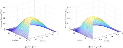
Figure 2. Numerical Solution of Example 7.2, with N = 64 = M. (a) $\epsilon =2^{-4}$ (b) $\epsilon =2^{-14}$.

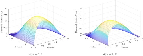
Figure 3. Numerical Solution of Example 7.3, with N = 64. (a) $\epsilon =2^{-8}$.

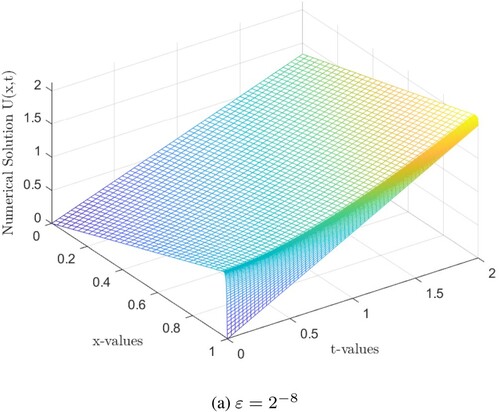
Table 1. $E_{\epsilon }^{N,\mathrm{\Delta t}},P_{\epsilon }^{N,\mathrm{\Delta t}},E^{N,\mathrm{\Delta t}},P^{N,\mathrm{\Delta t}}$, for Example 7.1 on Bakhvalov–Shishkin mesh.

$\epsilon \downarrow$	N = 32	$N=64$	$N=128$	N = 256	N = 512
	M = 40	M = 80	$M=160$	$M=320$	$M=640$
Before Richardson extrapolation
$2^{-12}$	3.6393e−03	2.0741e−03	1.2601e−03	7.1707e−04	3.8423e−04
$2^{-14}$	3.6366e−03	2.0736e−03	1.2545e−03	7.1481e−04	3.8334e−04
$2^{-16}$	3.6359e−03	2.0735e−03	1.2531e−03	7.1422e−04	3.8309e−04
$2^{-18}$	3.6358e−03	2.0735e−03	1.2527e−03	7.1407e−04	3.8303e−04
$2^{-20}$	3.6357e−03	2.0735e−03	1.2527e−03	7.1403e−04	3.8301e−04
$2^{-22}$	3.6357e−03	2.0735e−03	1.2526e−03	7.1402e−04	3.8301e−04
$2^{-24}$	3.6357e−03	2.0735e−03	1.2526e−03	7.1402e−04	3.8301e−04
$2^{-26}$	3.6357e−03	2.0735e−03	1.2526e−03	7.1402e−04	3.8301e−04
$2^{-28}$	3.6357e−03	2.0735e−03	1.2526e−03	7.1402e−04	3.8301e−04
$2^{-30}$	3.6357e−03	2.0735e−03	1.2526e−03	7.1402e−04	3.8301e−04
$2^{-32}$	3.6357e−03	2.0735e−03	1.2526e−03	7.1402e−04	3.8301e−04
$E^{N,\mathrm{\Delta t}}$	3.6393e−03	2.0741e−03	1.2601e−03	7.1707e−04	3.8423e−04
$P^{N,\mathrm{\Delta t}}$	0.8112	0.7190	0.8133	0.9001	–
After Richardson extrapolation
$2^{-12}$	3.1195e−03	9.3315e−04	2.7076e−04	7.6430e−05	2.1047e−05
$2^{-14}$	3.1500e−03	9.4711e−04	2.7683e−04	7.8930e−05	2.2018e−05
$2^{-16}$	3.1578e−03	9.5072e−04	2.7845e−04	7.9637e−05	2.2325e−05
$2^{-18}$	3.1598e−03	9.5163e−04	2.7886e−04	7.9820e−05	2.2407e−05
$2^{-20}$	3.1602e−03	9.5186e−04	2.7896e−04	7.9866e−05	2.2428e−05
$2^{-22}$	3.1604e−03	9.5192e−04	2.7899e−04	7.9877e−05	2.2433e−05
$2^{-24}$	3.1604e−03	9.5193e−04	2.7899e−04	7.9880e−05	2.2434e−05
$2^{-26}$	3.1604e−03	9.5193e−04	2.7899e−04	7.9880e−05	2.2435e−05
$2^{-28}$	3.1604e−03	9.5194e−04	2.7899e−04	7.9881e−05	2.2435e−05
$2^{-30}$	3.1604e−03	9.5194e−04	2.7900e−04	7.9884e−05	2.2439e−05
$2^{-32}$	3.1604e−03	9.5195e−04	2.7899e−04	7.9874e−05	2.2441e−05
$E_{\mathrm{ext}}^{N,\mathrm{\Delta t}}$	3.1604e−03	9.5195e−04	2.7900e−04	7.9884e−05	2.2441e−05
$P_{\mathrm{ext}}^{N,\mathrm{\Delta t}}$	1.7312	1.7706	1.8043	1.8318	–

Table 2. $E_{\epsilon }^{N,\mathrm{\Delta t}},P_{\epsilon }^{N,\mathrm{\Delta t}},E^{N,\mathrm{\Delta t}},P^{N,\mathrm{\Delta t}}$, for Example 7.2 on Bakhvalov–Shishkin mesh,with N = M.

$\epsilon \downarrow$	N = 16	N = 32	N = 64	N = 128	N = 256	N = 512
Before Richardson extrapolation
$2^{-14}$	7.2870e−03	3.1938e−03	1.6513e−03	9.2133e−04	4.8183e−04	2.4447e−04
$2^{-16}$	7.3001e−03	3.2027e−03	1.6588e−03	9.2875e−04	4.8900e−04	2.4984e−04
$2^{-18}$	7.3033e−03	3.2050e−03	1.6607e−03	9.3064e−04	4.9087e−04	2.5167e−04
$2^{-20}$	7.3041e−03	3.2055e−03	1.6611e−03	9.3112e−04	4.9134e−04	2.5213e−04
$2^{-22}$	7.3043e−03	3.2057e−03	1.6613e−03	9.3124e−04	4.9146e−04	2.5225e−04
$2^{-24}$	7.3044e−03	3.2057e−03	1.6613e−03	9.3127e−04	4.9149e−04	2.5228e−04
$2^{-26}$	7.3044e−03	3.2057e−03	1.6613e−03	9.3128e−04	4.9150e−04	2.5229e−04
$2^{-28}$	7.3044e−03	3.2057e−03	1.6613e−03	9.3128e−04	4.9150e−04	2.5229e−04
$2^{-30}$	7.3044e−03	3.2057e−03	1.6613e−03	9.3128e−04	4.9150e−04	2.5229e−04
$E^{N,\mathrm{\Delta t}}$	7.3044e−03	3.2057e−03	1.6613e−03	9.3128e−04	4.9150e−04	2.5229e−04
$P^{N,\mathrm{\Delta t}}$	1.1881	0.9483	0.8350	0.9220	0.9621	–
After Richardson extrapolation
$2^{-14}$	3.1941e−03	1.0609e−03	3.2872e−04	9.7039e−05	2.7660e−05	7.6726e−06
$2^{-16}$	3.1988e−03	1.0635e−03	3.3004e−04	9.7655e−05	2.7941e−05	7.8011e−06
$2^{-18}$	3.2000e−03	1.0642e−03	3.3037e−04	9.7809e−05	2.8012e−05	7.8330e−06
$2^{-20}$	3.2003e−03	1.0644e−03	3.3046e−04	9.7847e−05	2.8029e−05	7.8410e−06
$2^{-22}$	3.2003e−03	1.0644e−03	3.3048e−04	9.7857e−05	2.8034e−05	7.8430e−06
$2^{-24}$	3.2003e−03	1.0644e−03	3.3048e−04	9.7859e−05	2.8035e−05	7.8435e−06
$2^{-26}$	3.2003e−03	1.0644e−03	3.3048e−04	9.7860e−05	2.8035e−05	7.8436e−06
$2^{-28}$	3.2003e−03	1.0644e−03	3.3049e−04	9.7860e−05	2.8035e−05	7.8437e−06
$2^{-30}$	3.2003e−03	1.0644e−03	3.3049e−04	9.7861e−05	2.8037e−05	7.8446e−06
$E_{\mathrm{ext}}^{N,\mathrm{\Delta t}}$	3.2003e−03	1.0644e−03	3.3049e−04	9.7861e−05	2.8037e−05	7.8446e−06
$P_{\mathrm{ext}}^{N,\mathrm{\Delta t}}$	1.5882	1.6874	1.7558	1.8034	1.8376	–

Table 3. $E_{\epsilon }^{N,\mathrm{\Delta t}},P_{\epsilon }^{N,\mathrm{\Delta t}},E^{N,\mathrm{\Delta t}},P^{N,\mathrm{\Delta t}}$, for Example 7.3 on Bakhvalov–Shishkin mesh,with N = M.

$\epsilon \downarrow$	N = 16	N = 32	N = 64	N = 128	N = 256	N = 512
Before Richardson extrapolation
$2^{-14}$	1.63540e−02	7.99370e−03	3.95110e−03	1.96410e−03	9.79190e−04	4.88880e−04
$2^{-16}$	1.63570e−02	7.99510e−03	3.95180e−03	1.96450e−03	9.79360e−04	4.88970e−04
$2^{-18}$	1.63570e−02	7.99550e−03	3.95200e−03	1.96450e−03	9.79410e−04	4.88990e−04
$2^{-20}$	1.63570e−02	7.99560e−03	3.95200e−03	1.96460e−03	9.79420e−04	4.88990e−04
$2^{-22}$	1.63570e−02	7.99560e−03	3.95200e−03	1.96460e−03	9.79420e−04	4.89000e−04
$2^{-24}$	1.63570e−02	7.99560e−03	3.95200e−03	1.96460e−03	9.79420e−04	4.89000e−04
$2^{-26}$	1.63570e−02	7.99560e−03	3.95200e−03	1.96460e−03	9.79420e−04	4.89000e−04
$2^{-28}$	1.63570e−02	7.99560e−03	3.95200e−03	1.96460e−03	9.79420e−04	4.89000e−04
$2^{-30}$	1.63570e−02	7.99560e−03	3.95200e−03	1.96460e−03	9.79410e−04	4.89000e−04
$E^{N,\mathrm{\Delta t}}$	1.63570e−02	7.99560e−03	3.95200e−03	1.96460e−03	9.79420e−04	4.89000e−04
$P^{N,\mathrm{\Delta t}}$	1.0327	1.0166	1.0084	1.0042	1.0021	–
After Richardson extrapolation
$2^{-20}$	1.1216e−03	3.2191e−04	8.5972e−05	2.2231e−05	5.6865e−06	1.4732e−06
$2^{-22}$	1.1215e−03	3.2188e−04	8.5933e−05	2.2192e−05	5.6464e−06	1.4328e−06
$2^{-24}$	1.1215e−03	3.2187e−04	8.5923e−05	2.2182e−05	5.6363e−06	1.4227e−06
$2^{-26}$	1.1215e−03	3.2187e−04	8.5921e−05	2.2179e−05	5.6338e−06	1.4202e−06
$2^{-28}$	1.1215e−03	3.2187e−04	8.5920e−05	2.2179e−05	5.6332e−06	1.4196e−06
$2^{-30}$	1.1215e−03	3.2186e−04	8.5920e−05	2.2179e−05	5.6330e−06	1.4194e−06
$E_{\mathrm{ext}}^{N,\mathrm{\Delta t}}$	1.1216e−03	3.2191e−04	8.5972e−05	2.2231e−05	5.6865e−06	1.4732e−06
$P_{\mathrm{ext}}^{N,\mathrm{\Delta t}}$	1.8008	1.9047	1.9513	1.967	1.9486	–

Tables 4 and 5 display that, as values of ε goes to zero, the proposed scheme does not achieve uniform convergence if we use uniform mesh,as the error $E_{\epsilon }^{N,\mathrm{\Delta t}}$(and also $E^{N,\mathrm{\Delta t}}$) increase when the number of mesh points increases. This drawback is solved by using one of the Shishkin type mesh called Bakhvalov–Shishkin mesh.

Table 4. $E_{\epsilon }^{N,\mathrm{\Delta t}},E^{N,\mathrm{\Delta t}}$, for Example 7.1 on Uniform mesh with ${\lambda }_1=1/12$ and ${\lambda }_2=5/12$.

$\epsilon \downarrow$	N = 16	N = 32	$N=64$	N = 128	$N=256$	N = 512
	M = 20	M = 40	M = 80	M = 160	M = 320	M = 640
$2^{-4}$	7.6851e−03	1.8001e−03	9.2424e−04	4.7309e−04	2.3985e−04	1.2081e−04
$2^{-8}$	4.1614e−01	2.4193e−01	1.1678e−01	3.9420e−02	9.4794e−03	2.0822e−03
$2^{-12}$	8.1993e−01	7.9584e−01	6.5128e−01	5.2501e−01	4.0498e−01	2.5430e−01
$2^{-16}$	8.6028e−01	9.1966e−01	9.3446e−01	8.8004e−01	7.4237e−01	6.6215e−01
$2^{-20}$	8.6288e−01	9.2858e−01	9.6553e−01	9.8053e−01	9.6949e−01	9.0382e−01
$2^{-24}$	8.6305e−01	9.2914e−01	9.6756e−01	9.8809e−01	9.9757e−01	9.9747e−01
$2^{-28}$	8.6306e−01	9.2917e−01	9.6769e−01	9.8857e−01	9.9941e−01	1.0047e+00
$E^{N,\mathrm{\Delta t}}$	8.6306e−01	9.2917e−01	9.6769e−01	9.8857e−01	9.9941e−01	1.0047e+00

Table 5. $E_{\epsilon }^{N,\mathrm{\Delta t}},E^{N,\mathrm{\Delta t}}$, for Example 7.2 on Uniform mesh with ${\lambda }_1=1/12$, ${\lambda }_2=5/12$ and $N=M$.

$\epsilon \downarrow$	N = 16	N = 32	$N=64$	$N=128$	N = 256	N = 512
$2^{-4}$	2.3921e−03	1.2926e−03	6.8897e−04	3.5867e−04	1.8315e−04	9.2628e−05
$2^{-8}$	1.0978e−01	7.7038e−02	3.8786e−02	1.3359e−02	3.2354e−03	6.9549e−04
$2^{-12}$	1.8478e−01	2.0408e−01	2.0053e−01	1.7868e−01	1.3950e−01	8.8087e−02
$2^{-16}$	1.9115e−01	2.2046e−01	2.3694e−01	2.4244e−01	2.3812e−01	2.2925e−01
$2^{-20}$	1.9155e−01	2.2153e−01	2.3967e−01	2.4946e−01	2.5378e−01	2.5361e−01
$2^{-24}$	1.9158e−01	2.2160e−01	2.3984e−01	2.4993e−01	2.5515e−01	2.5765e−01
$2^{-28}$	1.9158e−01	2.2160e−01	2.3985e−01	2.4996e−01	2.5524e−01	2.5794e−01
$E^{N,\mathrm{\Delta t}}$	1.9158e−01	2.2160e−01	2.3985e−01	2.4996e−01	2.5524e−01	2.5794e−01

Table 6. Comparison of $E_{\epsilon }^{N,\mathrm{\Delta t}}$ for Example 7.1 when N = M.

$\epsilon \downarrow$	N = 32	N = 64	N = 128	N = 256	N = 512
Proposed method
$2^{-6}$	4.4584e−03	2.9063e−03	1.6488e−03	9.4635e−04	8.8529e−04
$2^{-8}$	3.7809e−03	2.5402e−03	1.7113e−03	1.1520e−03	8.2689e−04
$2^{-10}$	3.8301e−03	2.1723e−03	1.3360e−03	7.8317e−04	4.9180e−04
$2^{-12}$	4.0055e−03	2.2524e−03	1.3159e−03	7.4830e−04	4.0089e−04
$2^{-14}$	4.0509e−03	2.2830e−03	1.3102e−03	7.4604e−04	4.0000e−04
$2^{-16}$	4.0623e−03	2.2916e−03	1.3088e−03	7.4545e−04	3.9975e−04
$2^{-18}$	4.0652e−03	2.2937e−03	1.3084e−03	7.4529e−04	3.9969e−04
$2^{-20}$	4.0659e−03	2.2943e−03	1.3083e−03	7.4526e−04	3.9967e−04
$2^{-24}$	4.0662e−03	2.2944e−03	1.3083e−03	7.4524e−04	3.9967e−04
$2^{-26}$	4.0662e−03	2.2945e−03	1.3083e−03	7.4524e−04	3.9967e−04
$2^{-30}$	4.0662e−03	2.2945e−03	1.3083e−03	7.4524e−04	3.9966e−04
Method in [57]
$2^{-6}$	3.3040e−03	1.1073e−03	4.1432e−04	1.7826e−04	8.4960e−05
$2^{-8}$	7.1097e−03	3.0887e−03	9.6542e−04	3.1847e−04	1.1859e−04
$2^{-10}$	7.2307e−03	3.8516e−03	1.9512e−03	8.0308e−04	2.5301e−04
$2^{-12}$	7.2307e−03	3.8523e−03	1.9892e−03	1.0105e−03	4.9936e−04
$2^{-14}$	7.2307e−03	3.8523e−03	1.9892e−03	1.0107e−03	5.0944e−04
$2^{-16}$	7.2307e−03	3.8523e−03	1.9892e−03	1.0107e−03	5.0944e−04
$2^{-18}$	7.2307e−03	3.8523e−03	1.9892e−03	1.0107e−03	5.0944e−04
$2^{-20}$	7.2307e−03	3.8523e−03	1.9892e−03	1.0107e−03	5.0944e−04
$2^{-24}$	7.2307e−03	3.8523e−03	1.9892e−03	1.0107e−03	5.0944e−04
$2^{-26}$	7.2307e−03	3.8523e−03	1.9892e−03	1.0107e−03	5.0944e−04
$2^{-30}$	7.2307e−03	3.8523e−03	1.9892e−03	1.0107e−03	5.0944e−04

Table 7. Comparison of $E_{\epsilon }^{N,\mathrm{\Delta t}}$ for Example 7.2 when N = M.

$\epsilon \downarrow$	N = 16	N = 32	N = 64	N = 128	N = 256	N = 512
Proposed method
$2^{-14}$	7.2870e−03	3.1938e−03	1.6513e−03	9.2133e−04	4.8183e−04	2.4447e−04
$2^{-16}$	7.3001e−03	3.2027e−03	1.6588e−03	9.2875e−04	4.8900e−04	2.4984e−04
$2^{-18}$	7.3033e−03	3.2050e−03	1.6607e−03	9.3064e−04	4.9087e−04	2.5167e−04
$2^{-20}$	7.3041e−03	3.2055e−03	1.6611e−03	9.3112e−04	4.9134e−04	2.5213e−04
$2^{-22}$	7.3043e−03	3.2057e−03	1.6613e−03	9.3124e−04	4.9146e−04	2.5225e−04
$2^{-24}$	7.3044e−03	3.2057e−03	1.6613e−03	9.3127e−04	4.9149e−04	2.5228e−04
$2^{-26}$	7.3044e−03	3.2057e−03	1.6613e−03	9.3128e−04	4.9150e−04	2.5229e−04
$2^{-28}$	7.3044e−03	3.2057e−03	1.6613e−03	9.3128e−04	4.9150e−04	2.5229e−04
Method in [58]
$2^{-14}$	4.9006e−02	2.8622e−02	1.5141e−02	7.7173e−03	3.8858e−03	1.9484e−03
$2^{-16}$	4.9006e−02	2.8622e−02	1.5141e−02	7.7173e−03	3.8858e−03	1.9484e−03
$2^{-18}$	4.9006e−02	2.8622e−02	1.5141e−02	7.7173e−03	3.8858e−03	1.9484e−03
$2^{-20}$	4.9006e−02	2.8622e−02	1.5141e−02	7.7173e−03	3.8858e−03	1.9484e−03
$2^{-22}$	4.9006e−02	2.8622e−02	1.5141e−02	7.7173e−03	3.8858e−03	1.9484e−03
$2^{-24}$	4.9006e−02	2.8622e−02	1.5141e−02	7.7173e−03	3.8858e−03	1.9484e−03
$2^{-26}$	4.9006e−02	2.8622e−02	1.5141e−02	7.7173e−03	3.8858e−03	1.9484e−03
$2^{-28}$	4.9006e−02	2.8622e−02	1.5141e−02	7.7173e−03	3.8858e−03	1.9484e−03

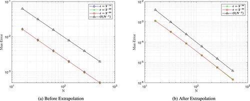
The maximum point wise errors for the solutions also plotted on log–log scale in Figures 4, 5, and 6, before and after extrapolation. The straight line that the plots follow demonstrates to us that one variable changes as a constant power of another; the maximum absolute point-wise error changes as a constant power of mesh parameter N. In addition, according to the negative slope, the maximum absolute error decreases as the number of grid points rises. In these figures the plots are parallel and overlap as $\epsilon \to 0$. This shows that the proposed scheme converges regardless of the value of the perturbation parameter ε. Further, we note that all computations have been performed using MATLAB^® R2022b software.

Figure 4. log–log plot of maximum point wise error for Example 7.1. (a) Before Extrapolation (b) After Extrapolation.

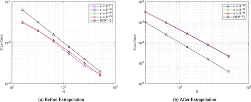
Figure 5. log–log plot of maximum point wise error for Example 7.2 (a) Before Extrapolation (b) After Extrapolation.

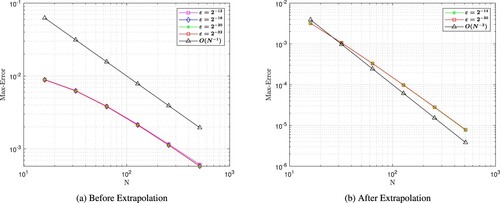
Figure 6. log–log plot of maximum point wise error for Example 7.3 (a) Before Extrapolation (b) After Extrapolation.

8. Conclusion

A numerical scheme for solving a class of singularly perturbed delay parabolic partial differential equations with Dirichlet boundary conditions is investigated. The scheme comprises implicit Euler for time discretization on uniform mesh and a hybrid scheme for spatial discretization on Bakhvalov–Shishkin mesh. The hybrid scheme is composed of midpoint upwind for coarse mesh and non-polynomial spline on fine mesh. Richardson extrapolation technique has been used to improve the accuracy of computed solutions and rate of convergence of the scheme. The delay term is treated by making the delay argument as one of nodal points. It has been shown that the present method is uniformly convergent with respect to the perturbation parameter ε and achieves second-order accuracy. Three test examples are presented that numerically validate the theoretical result. Further, it has been shown by the first two examples that the scheme is not convergent on a uniform mesh. The proposed method combined the unconditional stability and flexibility in choosing the basis function advantages from midpoint upwind and non-polynomial spline scheme respectively. These advantages are significant for solving singularly perturbed delay differential equations involving boundary layer phenomenon. Accordingly, as future directions of this research we extend the proposed scheme for solving time fractional singularly perturbed convection–diffusion problems with a delay in time.

Disclosure statement

No potential conflict of interest was reported by the author(s).

References

- Arino O, Hbid ML, Dads EA. Delay differential equations and applications: Proceedings of the nato advanced study institute held in marrakech, morocco: September 2002. Vol. 205. Springer Science & Business Media; 2007. p. 90–21.
- Murray JD. Mathematical biology: I an introduction. New York, NY: Springer; 2002.
- Wu J. Theory and applications of partial functional differential equations. Vol.119. New York: Springer Science & Business Media; 1996.
- Musila M, Lánskỳ P. Generalized stein's model for anatomically complex neurons. BioSystems. 1991;25(3):179–191. doi: 10.1016/0303-2647(91)90004-5
- Farrell P, Hegarty A, Miller JM, et al. Robust computational techniques for boundary layers. Boca Raton: Chapman and hall/CRC; 2000.
- Roos HG, Stynes M, Tobiska L. Robust numerical methods for singularly perturbed differential equations: convection–diffusion–reaction and flow problems. Vol. 24. Berlin, Heidelberg: Springer Science & Business Media; 2008.
- Singh J, Kumar S, Kumar M. A domain decomposition method for solving singularly perturbed parabolic reaction-diffusion problems with time delay. Numer Methods Partial Differ Equ. 2018;34(5):1849–1866. doi: 10.1002/num.v34.5
- Rao SCS, Kumar S. An almost fourth order uniformly convergent domain decomposition method for a coupled system of singularly perturbed reaction–diffusion equations. J Comput Appl Math. 2011;235(11):3342–3354. doi: 10.1016/j.cam.2011.01.047
- Kumar S. A parameter-uniform grid equidistribution method for singularly perturbed degenerate parabolic convection–diffusion problems. J Comput Appl Math. 2022;404:113273. doi: 10.1016/j.cam.2020.113273
- Kumar S, Kumar M. High order parameter-uniform discretization for singularly perturbed parabolic partial differential equations with time delay. Comput Math Appl. 2014;68(10):1355–1367. doi: 10.1016/j.camwa.2014.09.004
- Hailu WS, Duressa GF. Parameter-uniform cubic spline method for singularly perturbed parabolic differential equation with large negative shift and integral boundary condition. Res Math. 2022;9(1):2151080. doi: 10.1080/27684830.2022.2151080
- Hailu WS, Duressa GF. Uniformly convergent numerical method for singularly perturbed parabolic differential equations with non-smooth data and large negative shift. Res Math. 2022;9(1):2119677. doi: 10.1080/27684830.2022.2119677
- Kumar S. Layer-adapted methods for quasilinear singularly perturbed delay differential problems. Appl Math Comput. 2014;233:214–221.
- Hassen ZI, Duressa GF. New approach of convergent numerical method for singularly perturbed delay parabolic convection–diffusion problems. Res Math. 2023;10(1):2225267. doi: 10.1080/27684830.2023.2225267
- Hassen ZI, Duressa GF. Parameter-uniformly convergent numerical scheme for singularly perturbed delay parabolic differential equation via extended b-spline collocation. Front Appl Math Stat. 2023;9:1255672. doi: 10.3389/fams.2023.1255672
- Natividad MC, Stynes M. Richardson extrapolation for a convection–diffusion problem using a Shishkin mesh. Appl Numer Math. 2003;45(2-3):315–329. doi: 10.1016/S0168-9274(02)00212-X
- Mukherjee K, Natesan S. Richardson extrapolation technique for singularly perturbed parabolic convection–diffusion problems. Computing. 2011;92(1):1–32. doi: 10.1007/s00607-010-0126-8
- Clavero C, Gracia JL. A higher order uniformly convergent method with richardson extrapolation in time for singularly perturbed reaction–diffusion parabolic problems. J Comput Appl Math. 2013;252:75–85. doi: 10.1016/j.cam.2012.05.023
- Majumdar A, Natesan S. Second-order uniformly convergent richardson extrapolation method for singularly perturbed degenerate parabolic pdes. Int J Appl Comput Math. 2017;3(S1):31–53. doi: 10.1007/s40819-017-0380-y
- Negero NT, Duressa GF. An exponentially fitted spline method for singularly perturbed parabolic convection–diffusion problems with large time delay. Tamkang J Math. 2022;54:313–338.
- Negero NT, Duressa GF. Uniform convergent solution of singularly perturbed parabolic differential equations with general temporal-lag. Iran J Sci Technol, Trans A: Sci. 2022;46(2):507–524. doi: 10.1007/s40995-021-01258-2
- Megiso EA, Woldaregay MM, Dinka TG. Fitted tension spline method for singularly perturbed time delay reaction diffusion problems. Math Probl Eng. 2022;2022:1–10.doi: 10.1155/2022/8669718
- Kumar P, Ravi Kanth A. Computational study for a class of time-dependent singularly perturbed parabolic partial differential equation through tension spline. Comput Appl Math. 2020;39(1):1–19. doi: 10.1007/s40314-019-0964-8
- Ejere AH, Duressa GF, Woldaregay MM, et al. A uniformly convergent numerical scheme for solving singularly perturbed differential equations with large spatial delay. SN Appl Sci. 2022;4(12):324. doi: 10.1007/s42452-022-05203-9
- Rao RN, Chakravarthy PP. A fitted numerov method for singularly perturbed parabolic partial differential equation with a small negative shift arising in control theory. Numer Math: Theory, Methods Appl. 2014;7(1):23–40.
- Govindarao L, Mohapatra J. A second order numerical method for singularly perturbed delay parabolic partial differential equation. Eng Comput. 2018;36(2):420–444. doi: 10.1108/EC-08-2018-0337
- Niyogi P. Introduction to computational fluid dynamics. Don Mills: Pearson Education Canada; 2006.
- Das P, Mehrmann V. Numerical solution of singularly perturbed convection–diffusion–reaction problems with two small parameters. BIT Numerl Math. 2016;56:51–76. doi: 10.1007/s10543-015-0559-8
- Chandru M, Das P, Ramos H. Numerical treatment of two-parameter singularly perturbed parabolic convection diffusion problems with non-smooth data. Math Methods Appl Sci. 2018;41(14):5359–5387. doi: 10.1002/mma.v41.14
- Saini S, Das P, Kumar S. Computational cost reduction for coupled system of multiple scale reaction diffusion problems with mixed type boundary conditions having boundary layers. Rev De La Real Acad De Cienc Exactas, Fís Y Nat Serie A Mat. 2023;117(2):66. doi: 10.1007/s13398-023-01397-8
- Shiromani R, Shanthi V, Das P. A higher order hybrid-numerical approximation for a class of singularly perturbed two-dimensional convection–diffusion elliptic problem with non-smooth convection and source terms. Comput Math Appl. 2023;142:9–30. doi: 10.1016/j.camwa.2023.04.004
- Saini S, Das P, Kumar S. Parameter uniform higher order numerical treatment for singularly perturbed robin type parabolic reaction diffusion multiple scale problems with large delay in time. Appl Numer Math. 2024;196:1–21. doi: 10.1016/j.apnum.2023.10.003
- Das P, Rana S, Ramos H. On the approximate solutions of a class of fractional order nonlinear volterra integro-differential initial value problems and boundary value problems of first kind and their convergence analysis. J Comput Appl Math. 2022;404:113116. doi: 10.1016/j.cam.2020.113116
- Ladyzhenskaia OA, Solonnikov VA, Ural'tseva NN. Linear and quasi-linear equations of parabolic type. Vol. 23, Providence, RI: American Mathematical Soc.; 1968.
- Miller J, O'Riordan E, Shishkin G. Fitted numerical methods for singular perturbation problems: error estimates in the maximum norm for linear problems in one and two dimensions. Singapore: World Scientific; 2012.
- Das P, Rana S, Vigo-Aguiar J. Higher order accurate approximations on equidistributed meshes for boundary layer originated mixed type reaction diffusion systems with multiple scale nature. Appl Numer Math. 2020;148:79–97. doi: 10.1016/j.apnum.2019.08.028
- Das P, Rana S, Ramos H. A perturbation-based approach for solving fractional-order volterra–fredholm integro differential equations and its convergence analysis. Int J Comput Math. 2020;97(10):1994–2014. doi: 10.1080/00207160.2019.1673892
- Choudhary R, Singh S, Das P, et al. A higher order stable numerical approximation for time-fractional non-linear kuramoto–sivashinsky equation based on quintic b-spline. Math Methods Appl Sci. 2024. doi: 10.1002/mma.9778
- Negero NT, Duressa GF. A method of line with improved accuracy for singularly perturbed parabolic convection–diffusion problems with large temporal lag. Res Appl Math. 2021;11:100174. doi: 10.1016/j.rinam.2021.100174
- Das A, Natesan S. Uniformly convergent hybrid numerical scheme for singularly perturbed delay parabolic convection–diffusion problems on shishkin mesh. Appl Math Comput. 2015;271:168–186.
- Shishkin GI, Shishkina LP. Difference methods for singular perturbation problems. Boca Raton: Chapman and Hall/CRC; 2008.
- Linß T. An upwind difference scheme on a novel Shishkin-type mesh for a linear convection–diffusion problem. J Comput Appl Math. 1999;110(1):93–104. doi: 10.1016/S0377-0427(99)00198-3
- Ramesh V, Kadalbajoo MK. Upwind and midpoint upwind difference methods for time-dependent differential difference equations with layer behavior. Appl Math Comput. 2008;202(2):453–471.
- Stynes M, Roos HG. The midpoint upwind scheme. Appl Numer Math. 1997;23(3):361–374. doi: 10.1016/S0168-9274(96)00071-2
- Santra S, Mohapatra J, Das P, et al. Higher order approximations for fractional order integro-parabolic partial differential equations on an adaptive mesh with error analysis. Comput Math Appl. 2023;150:87–101. doi: 10.1016/j.camwa.2023.09.008
- Varga RS. Matrix iterative analysis. 2nd ed. Berlin: Springer; 2009. (Springer series in computational mathematics; 27).
- Woldaregay M, Duressa G. Exponentially fitted tension spline method for singularly perturbed differential difference equations. Iran J Numer Anal Optim. 2021;11(2):261–282.
- Kellogg T, Tsan A. Analysis of some difference approximations for a singular perturbation problem without turning points. Math Comput. 1978;32(144):1025–1039. doi: 10.1090/mcom/1978-32-144
- Das P. A higher order difference method for singularly perturbed parabolic partial differential equations. J Differ Equ Appl. 2018;24(3):452–477. doi: 10.1080/10236198.2017.1420792
- Das P. An a posteriori based convergence analysis for a nonlinear singularly perturbed system of delay differential equations on an adaptive mesh. Numer Algorithms. 2019;81(2):465–487. doi: 10.1007/s11075-018-0557-4
- Das P. Comparison of a priori and a posteriori meshes for singularly perturbed nonlinear parameterized problems. J Comput Appl Math. 2015;290:16–25. doi: 10.1016/j.cam.2015.04.034
- Das A, Govindarao L, Mohapatra J. A second order weighted monotone numerical scheme for time-delayed parabolic initial-boundary-value problem involving a small parameter. Int J Math Model Numer Optim. 2022;12(3):233–251.
- Bala S, Govindarao L, Das A, et al. Numerical scheme for partial differential equations involving small diffusion term with non-local boundary conditions. J Appl Math Comput. 2023;69(6):4307–4331. doi: 10.1007/s12190-023-01927-y
- Das A, Natesan S. Second-order uniformly convergent numerical method for singularly perturbed delay parabolic partial differential equations. Int J Comput Math. 2018;95(3):490–510. doi: 10.1080/00207160.2017.1290439
- Kumar K, Podila PC, Das P, et al. A graded mesh refinement approach for boundary layer originated singularly perturbed time-delayed parabolic convection diffusion problems. Math Methods Appl Sci. 2021;44(16):12332–12350. doi: 10.1002/mma.v44.16
- Kumar D. A parameter-uniform scheme for the parabolic singularly perturbed problem with a delay in time. Numer Methods Partial Differ Equ. 2021;37(1):626–642. doi: 10.1002/num.v37.1
- Negero N, Duressa G. An efficient numerical approach for singularly perturbed parabolic convection-diffusion problems with large time-lag. J Math Model. 2022;10(2):173–110.
- Babu G, Bansal K. A high order robust numerical scheme for singularly perturbed delay parabolic convection diffusion problems. J Appl Math Comput. 2022;68(1):363–389. doi: 10.1007/s12190-021-01512-1