Mathematical model of mosquito population dynamics with constants and periodic releases of Wolbachia-infected males

Abstract

In this article, we propose three mathematical models of mosquito dynamics. The first model describes the dynamics of wild mosquitoes in combination with mechanical control and larvicide. For this model, we derive a threshold parameter $\mathcal{N}$, called the basic number of offspring, and show that the trivial equilibrium is globally asymptotically stable when $\mathcal{N}\le 1$, while if $\mathcal{N}>1$, the non-trivial equilibrium is globally asymptotically stable. In the second model, we evaluated a constant release of Wolbachia-infected males in the wild mosquito population. Our analysis identified a critical threshold for releasing Wolbachia-infected male mosquitoes $M_i^{\mathrm{crit}}$ to reduce or eliminate the wild mosquito population. In the third model, we assessed wild mosquito dynamics by periodically releasing Wolbachia-infected male mosquitoes. The analysis of this model produced two thresholds, $T^{\ast }$ the threshold on the release period and ${\mathrm{\Lambda }}^{\ast }$ the threshold on the release quantity. The existence of trivial periodic solutions is obtained, and the corresponding local and global stability conditions are proved by Floquet's theory and Lyapunov's stability theorem, respectively. We also prove the existence conditions for non-trivial periodic solutions and their local stability. Finally, we perform some numerical simulations to illustrate our theoretically pertinent results.

Keywords:

• Basic offspring number
• stability
• vector control
• Wolbachia
• impulsive model
• periodic solutions

2020 Mathematics Subject Classifications:

• 65L12
• 65M20
• 65N40

1. Introduction

Mosquito-borne diseases are caused by bacteria, viruses or parasites transmitted by mosquitoes. Every year, nearly 700 million people suffer from mosquito-borne diseases, leading to more than a million deaths and a major economic burden in endemic countries [1]. In recent years, with global warming, ease of transportation and environmental degradation, the geographic environment suitable for mosquitoes has expanded, and various mosquito-borne diseases have continuously spread on a large scale. Anopheles, Aedes and Culex are three major mosquito genera, which comprise approximately $\mathrm{3,500}$ species, are found beyond the tropical and subtropical regions of the world. Different kinds of mosquitoes can transmit different pathogens. For example, Anopheles primarily transmit malaria and filariasis, Aedes can transmit Zika, dengue, yellow fever, and chikungunya, while Culex can transmit West Nile, Japanese encephalitis, and filariasis [2]. At present, there are no effective vaccines or therapeutic drugs to combat some mosquito-borne diseases, so controlling mosquito vectors has proven to be a suitable method to prevent the spread of transmitted diseases by mosquitoes [3–5]. However, excessive use of traditional methods to suppress the mosquito population is generally unhealthy or unsustainable for humans and the environment. For example, heavy use of chemical insecticides can lead to insecticide resistance and toxicological accumulation [3]. Thus, the search for new technologies aimed at breaking the cycle of transmission of diseases transmitted by mosquitoes has been applied in recent years. Notably, the Sterile Insect Technique (SIT) which is a method of biological insect control and requires the release of a large number of sterile insects into the wild. This technique was developed in the 1940s and 1950s and adopted for Anopheles, Culex, and Aedes mosquito control in the early 1970s and is now being utilized and accepted by some mosquito control programs. The released mosquitoes are preferably sterile males that compete with wild males to mate with females of the natural populations. After mating with a sterile male, females produce no offspring, thus reducing the next generation's population. This is an environmentally friendly control method involving mass-rearing and sterilization by radiation and other methods. In addition, we have the Cytoplasmic Incompatibility (CI) caused by endosymbiotic bacteria, Wolbachia [6]. Wolbachia is present in up to $60\mathrm{\%}$ of insect species including some mosquitoes. This bacterium induce cytoplasmic incompatibility (CI) in mosquitoes, which causes early embryonic mortality resulting from mating between Wolbachia-infected males and females which are either uninfected or infected with a different Wolbachia strain [7–9].

Mathematical models are useful tools for finding the best strategies in the implementation of different types of vector control interventions and for assessing their impact on the disease propagation [10–14]. Some authors had studies only one type of vector control interventions, such as insecticide spraying [15, 16], Sterile Insect Technique or SIT, [17–22], Wolbachia infestation [23–27] and introduction of natural predators of mosquito larvae [28, 29]. Others had focused on combinations of various types of vector control, namely, the combined effects of insecticide spraying with personal protection measures [30] or educational campaigns [31], interventions that complement the insecticide spraying with the use of larvicides [19, 21, 32, 33].

Our model is inspired by the work of [18, 33–35], by taking into account the total adult mosquito population in the mating process. Then, we introduce mechanical and larvicide control in the dynamics of the aquatic stage mosquitoes, combined with a constant and impulsive release of Wolbachia-infected males. Our main objective is to evaluate the impact of Wolbachia-infected male releases combined with mechanical and larvicidal control on the growth dynamics of wild mosquitoes. To achieve our objectives, we considered a simple model of the growth dynamics of mosquitoes combined with mechanical and larvicidal control and obtained a threshold $\mathcal{N}$. We then disrupted the dynamics of wild mosquitoes by releasing Wolbachia-infected males in a constant and impulsive manner.

The rest of the paper is organized as follows. In Section 2, we propose and analyse a mathematical model for the population dynamics of wild mosquitoes combined with mechanical control and larvicide treatment. This model was extended by considering a constant release of Wolbachia-infected male in Section 3. In addition, we present a qualitative analysis of this model. Specifically, we calculate the equilibria and study their stabilities. In Section 4, we establish an impulse model by periodically releasing Wolbachia-infected male mosquitoes. We then perform a dynamic analysis of the model to obtain the existence and stability of the periodic solution. In Section 5, we perform some numerical simulations to illustrate the results obtained. Finally, the conclusion of this paper is given in the last section.

2. Mathematical model of wild mosquito dynamics with mechanical and larvicide control

2.1. Mathematical formulation of the wild mosquito model

The life cycle of a mosquito consists of two main stages: aquatic (egg, larva, pupa) and adult (males and females). A few days after being fertilized, a female mosquito may deposit a few dozen eggs possibly divided between several breeding sites. Once laid, the eggs of some species can resist up to several months before hatching. After stimulation, the eggs hatch to give rise to larvae that will develop in the water and reach the stage of pupae. The larval stage lasts from a few days to a few weeks.

For the mathematical description, we consider two stages: the aquatic stage and adult stage. We denote by A the aquatic stage (egg, larva, pupa) and we divided the adult stage in three sub-compartments: M wild males, F young females not yet laying eggs, $F_s$ fertilized and egg-laying females. We consider that a female to be in the F compartment from its emergence from aquatic stage until her gonotrophic cycle has began, that is the time of mating and taking the first blood meal, which takes typically 3−4 days. The vector control terms added to the model are the application of larvicide (chemical control) and the removal of potential breeding sites (mechanical control). The description of the control terms is as follows:

• θ is defined as the parameter associated with the effectiveness of mechanical control, which consists of destroying the breeding sites.

• ω is the mortality rate caused by the use of the larvicide that will affect the aquatic stage of the mosquito population.

The life cycle is described using the diagram in Figure 1. The variables and parameters of the system are detailed in Tables 1 and 2, respectively, where we indicate each variable and each parameter of the system giving its physical meaning and its quasi-dimensional unity [36–39].

Figure 1. Wild mosquito flow chart.

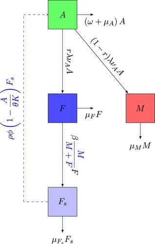
Table 1. Types of state variables and their quasi-dimensional unit which is either a for aquatic life stage and f for adult mosquitoes or terrestrial forms of the mosquito.

Type of variable	Description	Quasi-dimension
A	Aquatic stages of the mosquito and pupae	a
M	Wild male mosquitoes	f
F	Young females not yet laying eggs	f
$F_s$	Fertilized and egg-laying females	f

Table 2. Parameters of model (1(1) $\{\begin{array}{l}\dot{A}\left(t\right)=\mathrm{\rho \varphi }(1-{\displaystyle \frac{A\left(t\right)}{\mathrm{\theta K}}})F_s\left(t\right)-({\nu }_A+\omega +{\mu }_A)A\left(t\right),\\ \dot{M}\left(t\right)=(1-r)\lambda {\nu }_{A}A\left(t\right)-{\mu }_{M}M\left(t\right),\\ \dot{F}\left(t\right)=\mathrm{r\lambda }{\nu }_{A}A\left(t\right)-(\text{β}+{\mu }_F)F\left(t\right),\\ {\dot{F}}_s\left(t\right)=\text{β}{\displaystyle \frac{M\left(t\right)}{M\left(t\right)+F\left(t\right)}F\left(t\right)-{\mu }_{F_s}{F}_s\left(t\right),}\end{array}$(1) ), their description and corresponding quasi-dimension.

Symbol	Description	Quasi-dimension
${\nu }_A$	Rate of transition from aquatic to adult	${\mathrm{Time}}^{-1}$
ω	Mortality rate induced by larvicide	${\mathrm{Time}}^{-1}$
θ	The efficacy of the mechanical control	−−
${\mu }_A$	Natural death rate in the aquatic stade	${\mathrm{Time}}^{-1}$
K	Maximum number of aquatic mosquitoes that the medium supports	aquatic mosquitoes
${\mu }_M$	Death rate of wild male	${\mathrm{Time}}^{-1}$
β	Natural mating rate of a female by a male	${\mathrm{Time}}^{-1}$
${\mu }_F$	Death rate of young females not yet laying eggs	${\mathrm{Time}}^{-1}$
${\mu }_{F_s}$	Death rate of fertilized and egg-laying females	${\mathrm{Time}}^{-1}$
ϕ	The average amount of eggs laid per fertilized female	${\mathrm{Time}}^{-1}$
r	Sex ratio	−−
ρ	Bio-transition factor of oviposition per reproducing vector	${\mathrm{af}}^{-1}$
λ	Bio-transition factor to measure successful transition from aquatic to adult stage	${\mathrm{fa}}^{-1}$

Thus, the corresponding mathematical model is given by system (1(1) $\{\begin{array}{l}\dot{A}\left(t\right)=\mathrm{\rho \varphi }(1-{\displaystyle \frac{A\left(t\right)}{\mathrm{\theta K}}})F_s\left(t\right)-({\nu }_A+\omega +{\mu }_A)A\left(t\right),\\ \dot{M}\left(t\right)=(1-r)\lambda {\nu }_{A}A\left(t\right)-{\mu }_{M}M\left(t\right),\\ \dot{F}\left(t\right)=\mathrm{r\lambda }{\nu }_{A}A\left(t\right)-(\text{β}+{\mu }_F)F\left(t\right),\\ {\dot{F}}_s\left(t\right)=\text{β}{\displaystyle \frac{M\left(t\right)}{M\left(t\right)+F\left(t\right)}F\left(t\right)-{\mu }_{F_s}{F}_s\left(t\right),}\end{array}$(1) ): (1) $\{\begin{array}{l}\dot{A}\left(t\right)=\mathrm{\rho \varphi }(1-{\displaystyle \frac{A\left(t\right)}{\mathrm{\theta K}}})F_s\left(t\right)-({\nu }_A+\omega +{\mu }_A)A\left(t\right),\\ \dot{M}\left(t\right)=(1-r)\lambda {\nu }_{A}A\left(t\right)-{\mu }_{M}M\left(t\right),\\ \dot{F}\left(t\right)=\mathrm{r\lambda }{\nu }_{A}A\left(t\right)-(\text{β}+{\mu }_F)F\left(t\right),\\ {\dot{F}}_s\left(t\right)=\text{β}{\displaystyle \frac{M\left(t\right)}{M\left(t\right)+F\left(t\right)}F\left(t\right)-{\mu }_{F_s}{F}_s\left(t\right),}\end{array}$(1) with non-negative initial condition, (2) $A\left(0\right)=A_0,M\left(0\right)=M_0,F\left(0\right)=F_0,F_s\left(0\right)=F_{s0}.$(2) For, the variation of the population of male mosquitoes M, the inflow is $(1-r)\lambda {\nu }_{A}A$, which represents the number of mosquitoes that develop to male adults per unit of time and the outflow is represented by ${\mu }_{M}M$, which expresses the male mosquitoes that die per unit of time. For the variation of young females not yet laying eggs F, the inflow is $\mathrm{r\lambda }{\nu }_{A}A$, which indicates the number of mosquitoes that develop to young female adults. The parameter $1/(\text{β}+{\mu }_F)$ can represents the average time given by the length of a female's first gonotrophic cycle of a female, i.e. the interval between immediately after mating and the first blood meal [18]. As mating is a complex process, as indicated in [18, 40], the male mosquito can mate practically throughout his life. A female mosquito needs successful mating to reproduce throughout her life [18, 40]. Note that mosquitoes locate themselves in space and time to ensure they are available to mate. Thus, we consider that the total number of mosquitoes in the aerial phase is expressed by the term M + F, and the fraction $M/(M+F)$ represents the probability that a young females meets a male in the adult phase. Then, $\mathrm{MF}/(M+F)$ is the number of encounters between males and young females. So, $\text{β}\mathrm{MF}/(M+F)$ is the number of matings between young females and males per unit of time. ${\mu }_{F}F$ (resp. ${\mu }_s{F}_s$) is the number of young females (resp. fertilized and egg-laying females) mosquitoes that die per unit of time. $\mathrm{\rho \varphi }{F}_s$ represents the number of eggs per unit of time laid by fertilized and egg-laying females without considering the number of aquatic mosquitoes that the medium can support. $(1-A/\mathrm{\theta K})$ indicates the probability that there is a place available for more aquatic mosquitoes and $(\omega +{\mu }_A)A$ which represents the aquatic mosquitoes that die per unit of time.

2.2. Mathematical analysis of the wild mosquito model

In this section, we present some theoretical results of system (1(1) $\{\begin{array}{l}\dot{A}\left(t\right)=\mathrm{\rho \varphi }(1-{\displaystyle \frac{A\left(t\right)}{\mathrm{\theta K}}})F_s\left(t\right)-({\nu }_A+\omega +{\mu }_A)A\left(t\right),\\ \dot{M}\left(t\right)=(1-r)\lambda {\nu }_{A}A\left(t\right)-{\mu }_{M}M\left(t\right),\\ \dot{F}\left(t\right)=\mathrm{r\lambda }{\nu }_{A}A\left(t\right)-(\text{β}+{\mu }_F)F\left(t\right),\\ {\dot{F}}_s\left(t\right)=\text{β}{\displaystyle \frac{M\left(t\right)}{M\left(t\right)+F\left(t\right)}F\left(t\right)-{\mu }_{F_s}{F}_s\left(t\right),}\end{array}$(1) ). First, we present the basic properties of the solutions of system (1(1) $\{\begin{array}{l}\dot{A}\left(t\right)=\mathrm{\rho \varphi }(1-{\displaystyle \frac{A\left(t\right)}{\mathrm{\theta K}}})F_s\left(t\right)-({\nu }_A+\omega +{\mu }_A)A\left(t\right),\\ \dot{M}\left(t\right)=(1-r)\lambda {\nu }_{A}A\left(t\right)-{\mu }_{M}M\left(t\right),\\ \dot{F}\left(t\right)=\mathrm{r\lambda }{\nu }_{A}A\left(t\right)-(\text{β}+{\mu }_F)F\left(t\right),\\ {\dot{F}}_s\left(t\right)=\text{β}{\displaystyle \frac{M\left(t\right)}{M\left(t\right)+F\left(t\right)}F\left(t\right)-{\mu }_{F_s}{F}_s\left(t\right),}\end{array}$(1) ). These are useful for showing that system (1(1) $\{\begin{array}{l}\dot{A}\left(t\right)=\mathrm{\rho \varphi }(1-{\displaystyle \frac{A\left(t\right)}{\mathrm{\theta K}}})F_s\left(t\right)-({\nu }_A+\omega +{\mu }_A)A\left(t\right),\\ \dot{M}\left(t\right)=(1-r)\lambda {\nu }_{A}A\left(t\right)-{\mu }_{M}M\left(t\right),\\ \dot{F}\left(t\right)=\mathrm{r\lambda }{\nu }_{A}A\left(t\right)-(\text{β}+{\mu }_F)F\left(t\right),\\ {\dot{F}}_s\left(t\right)=\text{β}{\displaystyle \frac{M\left(t\right)}{M\left(t\right)+F\left(t\right)}F\left(t\right)-{\mu }_{F_s}{F}_s\left(t\right),}\end{array}$(1) ) is well posed mathematically and biologically. Indeed, note that system (1(1) $\{\begin{array}{l}\dot{A}\left(t\right)=\mathrm{\rho \varphi }(1-{\displaystyle \frac{A\left(t\right)}{\mathrm{\theta K}}})F_s\left(t\right)-({\nu }_A+\omega +{\mu }_A)A\left(t\right),\\ \dot{M}\left(t\right)=(1-r)\lambda {\nu }_{A}A\left(t\right)-{\mu }_{M}M\left(t\right),\\ \dot{F}\left(t\right)=\mathrm{r\lambda }{\nu }_{A}A\left(t\right)-(\text{β}+{\mu }_F)F\left(t\right),\\ {\dot{F}}_s\left(t\right)=\text{β}{\displaystyle \frac{M\left(t\right)}{M\left(t\right)+F\left(t\right)}F\left(t\right)-{\mu }_{F_s}{F}_s\left(t\right),}\end{array}$(1) ) can be written in matrix form as follows: (3) $\dot{X}=P\left(X\right)X,$(3) where $X=(A,M,F,F_s{)}^T$ and $P\left(X\right)=\left(\begin{array}{cccc}-\left({\displaystyle \frac{\mathrm{\rho \varphi }{F}_s}{\mathrm{\theta K}}+{\nu }_A+\omega +{\mu }_A}\right)& 0& 0& \varphi \\ (1-r)\lambda {\nu }_A& -{\mu }_M& 0& 0\\ \mathrm{r\lambda }{\nu }_A& 0& -(\text{β}+{\mu }_F)& 0\\ 0& 0& {\displaystyle \frac{\text{β}M}{M+F}}& -{\mu }_{F_s}\end{array}\right)$The right-hand side of system (1(1) $\{\begin{array}{l}\dot{A}\left(t\right)=\mathrm{\rho \varphi }(1-{\displaystyle \frac{A\left(t\right)}{\mathrm{\theta K}}})F_s\left(t\right)-({\nu }_A+\omega +{\mu }_A)A\left(t\right),\\ \dot{M}\left(t\right)=(1-r)\lambda {\nu }_{A}A\left(t\right)-{\mu }_{M}M\left(t\right),\\ \dot{F}\left(t\right)=\mathrm{r\lambda }{\nu }_{A}A\left(t\right)-(\text{β}+{\mu }_F)F\left(t\right),\\ {\dot{F}}_s\left(t\right)=\text{β}{\displaystyle \frac{M\left(t\right)}{M\left(t\right)+F\left(t\right)}F\left(t\right)-{\mu }_{F_s}{F}_s\left(t\right),}\end{array}$(1) ) is continuous and infinitely differentiable on ${\mathbb{R}}_{+}^4$. Therefore, it is locally Lipschitz on ${\mathbb{R}}_{+}^4$, which guarantees the existence and uniqueness of the solution of system (1(1) $\{\begin{array}{l}\dot{A}\left(t\right)=\mathrm{\rho \varphi }(1-{\displaystyle \frac{A\left(t\right)}{\mathrm{\theta K}}})F_s\left(t\right)-({\nu }_A+\omega +{\mu }_A)A\left(t\right),\\ \dot{M}\left(t\right)=(1-r)\lambda {\nu }_{A}A\left(t\right)-{\mu }_{M}M\left(t\right),\\ \dot{F}\left(t\right)=\mathrm{r\lambda }{\nu }_{A}A\left(t\right)-(\text{β}+{\mu }_F)F\left(t\right),\\ {\dot{F}}_s\left(t\right)=\text{β}{\displaystyle \frac{M\left(t\right)}{M\left(t\right)+F\left(t\right)}F\left(t\right)-{\mu }_{F_s}{F}_s\left(t\right),}\end{array}$(1) ) associated with the initial conditions $X\left(0\right)=X_0\in {\mathbb{R}}_{+}^4$.

We have the following result.

Proposition 2.1

The set $\mathrm{\Omega }=\{X\in {\mathbb{R}}_{+}^4:A\le \mathrm{\theta K},M\le \frac{(1-r)\lambda {\nu }_A\mathrm{\theta K}}{{\mu }_M},F\le \frac{\mathrm{r\lambda }{\nu }_A\mathrm{\theta K}}{\text{β}+{\mu }_F},F_s\le \frac{\mathrm{r\lambda }{\nu }_A\text{β}\mathrm{\theta K}}{{\mu }_{F_s}(\text{β}+{\mu }_F)}\}$is positively invariant for system (1(1) $\{\begin{array}{l}\dot{A}\left(t\right)=\mathrm{\rho \varphi }(1-{\displaystyle \frac{A\left(t\right)}{\mathrm{\theta K}}})F_s\left(t\right)-({\nu }_A+\omega +{\mu }_A)A\left(t\right),\\ \dot{M}\left(t\right)=(1-r)\lambda {\nu }_{A}A\left(t\right)-{\mu }_{M}M\left(t\right),\\ \dot{F}\left(t\right)=\mathrm{r\lambda }{\nu }_{A}A\left(t\right)-(\text{β}+{\mu }_F)F\left(t\right),\\ {\dot{F}}_s\left(t\right)=\text{β}{\displaystyle \frac{M\left(t\right)}{M\left(t\right)+F\left(t\right)}F\left(t\right)-{\mu }_{F_s}{F}_s\left(t\right),}\end{array}$(1) ).

Proof.

We prove it in two steps:

Step 1:

We show that the solution variables $\left(A\right(t),M(t),F(t),F_s(t\left)\right)$ of system (1(1) $\{\begin{array}{l}\dot{A}\left(t\right)=\mathrm{\rho \varphi }(1-{\displaystyle \frac{A\left(t\right)}{\mathrm{\theta K}}})F_s\left(t\right)-({\nu }_A+\omega +{\mu }_A)A\left(t\right),\\ \dot{M}\left(t\right)=(1-r)\lambda {\nu }_{A}A\left(t\right)-{\mu }_{M}M\left(t\right),\\ \dot{F}\left(t\right)=\mathrm{r\lambda }{\nu }_{A}A\left(t\right)-(\text{β}+{\mu }_F)F\left(t\right),\\ {\dot{F}}_s\left(t\right)=\text{β}{\displaystyle \frac{M\left(t\right)}{M\left(t\right)+F\left(t\right)}F\left(t\right)-{\mu }_{F_s}{F}_s\left(t\right),}\end{array}$(1) ) corresponding to initial conditions such that $A\left(0\right)>0,M\left(0\right)>0,F\left(0\right)>0$ and $F_s\left(0\right)>0$ are non-negative. Let $t_1=sup\{t>0/\mathrm{\forall }u\in [0,t]:A(u)>0,M(u)>0,F(u)>0,F_s(u)>0\}.$The initial conditions above in addition to the continuity of all functions A, M, F and $F_s$ guarantee the existence of $t_1$. If $t_1=+\mathrm{\infty }$, then all solutions of system (1(1) $\{\begin{array}{l}\dot{A}\left(t\right)=\mathrm{\rho \varphi }(1-{\displaystyle \frac{A\left(t\right)}{\mathrm{\theta K}}})F_s\left(t\right)-({\nu }_A+\omega +{\mu }_A)A\left(t\right),\\ \dot{M}\left(t\right)=(1-r)\lambda {\nu }_{A}A\left(t\right)-{\mu }_{M}M\left(t\right),\\ \dot{F}\left(t\right)=\mathrm{r\lambda }{\nu }_{A}A\left(t\right)-(\text{β}+{\mu }_F)F\left(t\right),\\ {\dot{F}}_s\left(t\right)=\text{β}{\displaystyle \frac{M\left(t\right)}{M\left(t\right)+F\left(t\right)}F\left(t\right)-{\mu }_{F_s}{F}_s\left(t\right),}\end{array}$(1) ) are positive. Suppose $t_1<+\mathrm{\infty }$, then there exists at least one solution $A\left(t\right),M\left(t\right),F\left(t\right)$ or $F_s\left(t\right)$ that is equal to zero at $t_1$. Suppose, for example that $A\left(t_1\right)=0$, then the first equation of system (1(1) $\{\begin{array}{l}\dot{A}\left(t\right)=\mathrm{\rho \varphi }(1-{\displaystyle \frac{A\left(t\right)}{\mathrm{\theta K}}})F_s\left(t\right)-({\nu }_A+\omega +{\mu }_A)A\left(t\right),\\ \dot{M}\left(t\right)=(1-r)\lambda {\nu }_{A}A\left(t\right)-{\mu }_{M}M\left(t\right),\\ \dot{F}\left(t\right)=\mathrm{r\lambda }{\nu }_{A}A\left(t\right)-(\text{β}+{\mu }_F)F\left(t\right),\\ {\dot{F}}_s\left(t\right)=\text{β}{\displaystyle \frac{M\left(t\right)}{M\left(t\right)+F\left(t\right)}F\left(t\right)-{\mu }_{F_s}{F}_s\left(t\right),}\end{array}$(1) ) yields $\dot{A}=\mathrm{\rho \varphi }{F}_s-(\frac{\mathrm{\rho \varphi }{F}_s}{\mathrm{\theta K}}+({\nu }_A+\omega +{\mu }_A))A$which may be rewritten as follows $\frac{\mathrm{d}}{\mathrm{d}t}\left[A\right(t)\exp ({\int }_0^t\frac{\mathrm{\rho \varphi }{F}_s\left(v\right)}{\mathrm{\theta K}}+\vartheta \mathrm{d}v)]=\mathrm{\rho \varphi }{F}_s\left(t\right)\exp ({\int }_0^t\frac{\mathrm{\rho \varphi }{F}_s\left(v\right)}{\mathrm{\theta K}}+\vartheta \mathrm{d}v),$with $\vartheta ={\nu }_A+\omega +{\mu }_A$.Integrating the above inequality from 0 to $t_1$ gives $\begin{array}{rl}A\left(t_1\right)& =\left[A\right(0)+{\displaystyle {\int }_0^{t_1}\mathrm{\rho \varphi }{F}_s\left(t\right)\exp ({\int }_0^t\frac{\mathrm{\rho \varphi }{F}_s\left(v\right)}{\mathrm{\theta K}}+\vartheta \mathrm{d}v)\mathrm{d}t}]\\ & \times \exp (-{\int }_0^{t_1}\frac{\mathrm{\rho \varphi }{F}_s\left(v\right)}{\mathrm{\theta K}}+\vartheta \mathrm{d}v)>0,\end{array}$which is in contradiction with $A\left(t_1\right)=0$. Similarly, one can show that $M\left(t_1\right)>0,F\left(t_1\right)>0$ and $F_s\left(t_1\right)>0$. Thus, $A\left(t\right)>0,M\left(t\right)>0,F\left(t\right)>0$ and $F_s\left(t\right)>0$ for all t>0.

Step 2:

From the first equation of system (1(1) $\{\begin{array}{l}\dot{A}\left(t\right)=\mathrm{\rho \varphi }(1-{\displaystyle \frac{A\left(t\right)}{\mathrm{\theta K}}})F_s\left(t\right)-({\nu }_A+\omega +{\mu }_A)A\left(t\right),\\ \dot{M}\left(t\right)=(1-r)\lambda {\nu }_{A}A\left(t\right)-{\mu }_{M}M\left(t\right),\\ \dot{F}\left(t\right)=\mathrm{r\lambda }{\nu }_{A}A\left(t\right)-(\text{β}+{\mu }_F)F\left(t\right),\\ {\dot{F}}_s\left(t\right)=\text{β}{\displaystyle \frac{M\left(t\right)}{M\left(t\right)+F\left(t\right)}F\left(t\right)-{\mu }_{F_s}{F}_s\left(t\right),}\end{array}$(1) ), we will show that $\mathrm{\forall t}>0,A\left(t\right)\le \mathrm{\theta K}$. Indeed, suppose that there exists $t_0>0$ such that $A\left(t_0\right)>\mathrm{\theta K}$. By continuity, there exists $t_1<t_0$ such that $A\left(t_1\right)=\mathrm{\theta K}$ and $\mathrm{\forall t}\in ]t_1,t_0]$, we have $A\left(t\right)>\mathrm{\theta K}$. Thus, if $A\left(t_1\right)=\mathrm{\theta K}$, from the first equation of system (1(1) $\{\begin{array}{l}\dot{A}\left(t\right)=\mathrm{\rho \varphi }(1-{\displaystyle \frac{A\left(t\right)}{\mathrm{\theta K}}})F_s\left(t\right)-({\nu }_A+\omega +{\mu }_A)A\left(t\right),\\ \dot{M}\left(t\right)=(1-r)\lambda {\nu }_{A}A\left(t\right)-{\mu }_{M}M\left(t\right),\\ \dot{F}\left(t\right)=\mathrm{r\lambda }{\nu }_{A}A\left(t\right)-(\text{β}+{\mu }_F)F\left(t\right),\\ {\dot{F}}_s\left(t\right)=\text{β}{\displaystyle \frac{M\left(t\right)}{M\left(t\right)+F\left(t\right)}F\left(t\right)-{\mu }_{F_s}{F}_s\left(t\right),}\end{array}$(1) ), we have (4) $\dot{A}\left(t_1\right)=-({\nu }_A+\omega +{\mu }_A)\mathrm{\theta K}<0.$(4) Then, there exists $t_2\in ]t_1,t_0[$ such that $A\left(t_2\right)<\mathrm{\theta K}$ which is absurd because $A\left(t\right)>\mathrm{\theta K},\mathrm{\forall t}\in ]t_1,t_0]$. Thus, for all t>0, we have $A\left(t\right)\le \mathrm{\theta K}$. Using the fact that $A\left(t\right)\le \mathrm{\theta K},\mathrm{\forall t}>0$, the second equation in system (1(1) $\{\begin{array}{l}\dot{A}\left(t\right)=\mathrm{\rho \varphi }(1-{\displaystyle \frac{A\left(t\right)}{\mathrm{\theta K}}})F_s\left(t\right)-({\nu }_A+\omega +{\mu }_A)A\left(t\right),\\ \dot{M}\left(t\right)=(1-r)\lambda {\nu }_{A}A\left(t\right)-{\mu }_{M}M\left(t\right),\\ \dot{F}\left(t\right)=\mathrm{r\lambda }{\nu }_{A}A\left(t\right)-(\text{β}+{\mu }_F)F\left(t\right),\\ {\dot{F}}_s\left(t\right)=\text{β}{\displaystyle \frac{M\left(t\right)}{M\left(t\right)+F\left(t\right)}F\left(t\right)-{\mu }_{F_s}{F}_s\left(t\right),}\end{array}$(1) ) gives (5) $\dot{M}\left(t\right)\le (1-r)\lambda {\nu }_A\mathrm{\theta K}-{\mu }_{M}M\left(t\right).$(5) Applying the Gronwall's theorem to Equation (5(5) $\dot{M}\left(t\right)\le (1-r)\lambda {\nu }_A\mathrm{\theta K}-{\mu }_{M}M\left(t\right).$(5) ), one has that $M\left(t\right)\le \frac{(1-r)\lambda {\nu }_A\mathrm{\theta K}}{{\mu }_M}+\left(M\right(0)-\frac{(1-r)\lambda {\nu }_A\mathrm{\theta K}}{{\mu }_M}){\mathrm{e}}^{-{\mu }_{M}t},$where $M\left(0\right)$ represents the initial value of $M\left(t\right)$. It then follows that ${\displaystyle \underset{t\to \mathrm{\infty }}{lim sup}M\left(t\right)\le \frac{(1-r)\lambda {\nu }_A\mathrm{\theta K}}{{\mu }_M},\mathrm{therefore}M\left(t\right)\le \frac{(1-r)\lambda {\nu }_A\mathrm{\theta K}}{{\mu }_M}\text{for all}t>0.}$Using the fact that $A\left(t\right)\le \mathrm{\theta K},\mathrm{\forall t}>0$, the third equation in system (1(1) $\{\begin{array}{l}\dot{A}\left(t\right)=\mathrm{\rho \varphi }(1-{\displaystyle \frac{A\left(t\right)}{\mathrm{\theta K}}})F_s\left(t\right)-({\nu }_A+\omega +{\mu }_A)A\left(t\right),\\ \dot{M}\left(t\right)=(1-r)\lambda {\nu }_{A}A\left(t\right)-{\mu }_{M}M\left(t\right),\\ \dot{F}\left(t\right)=\mathrm{r\lambda }{\nu }_{A}A\left(t\right)-(\text{β}+{\mu }_F)F\left(t\right),\\ {\dot{F}}_s\left(t\right)=\text{β}{\displaystyle \frac{M\left(t\right)}{M\left(t\right)+F\left(t\right)}F\left(t\right)-{\mu }_{F_s}{F}_s\left(t\right),}\end{array}$(1) ) gives (6) $\dot{F}\left(t\right)\le \mathrm{r\lambda }{\nu }_A\mathrm{\theta K}-(\text{β}+{\mu }_F)F\left(t\right).$(6) Applying the Gronwall's theorem to Equation (6(6) $\dot{F}\left(t\right)\le \mathrm{r\lambda }{\nu }_A\mathrm{\theta K}-(\text{β}+{\mu }_F)F\left(t\right).$(6) ), one has that $F\left(t\right)\le \frac{\mathrm{r\lambda }{\nu }_A\mathrm{\theta K}}{\text{β}+{\mu }_F}+\left(F\right(0)-\frac{\mathrm{r\lambda }{\nu }_A\mathrm{\theta K}}{\text{β}+{\mu }_F}){\mathrm{e}}^{-(\text{β}+{\mu }_F)t},$where $F\left(0\right)$ represents the initial value of $F\left(t\right)$. It then follows that ${\displaystyle \underset{t\to \mathrm{\infty }}{lim sup}F\left(t\right)\le \frac{\mathrm{r\lambda }{\nu }_A\mathrm{\theta K}}{\text{β}+{\mu }_F},\mathrm{therefore}F\left(t\right)\le \frac{\mathrm{r\lambda }{\nu }_A\mathrm{\theta K}}{\text{β}+{\mu }_F}\text{for all}t>0.}$Now, using the fact that $F\left(t\right)\le \frac{\mathrm{r\lambda }{\nu }_A\mathrm{\theta K}}{\text{β}+{\mu }_F}$ for all t>0, the fourth equation in system (1(1) $\{\begin{array}{l}\dot{A}\left(t\right)=\mathrm{\rho \varphi }(1-{\displaystyle \frac{A\left(t\right)}{\mathrm{\theta K}}})F_s\left(t\right)-({\nu }_A+\omega +{\mu }_A)A\left(t\right),\\ \dot{M}\left(t\right)=(1-r)\lambda {\nu }_{A}A\left(t\right)-{\mu }_{M}M\left(t\right),\\ \dot{F}\left(t\right)=\mathrm{r\lambda }{\nu }_{A}A\left(t\right)-(\text{β}+{\mu }_F)F\left(t\right),\\ {\dot{F}}_s\left(t\right)=\text{β}{\displaystyle \frac{M\left(t\right)}{M\left(t\right)+F\left(t\right)}F\left(t\right)-{\mu }_{F_s}{F}_s\left(t\right),}\end{array}$(1) ) gives (7) ${\dot{F}}_s\left(t\right)\le \text{β}\frac{\mathrm{r\lambda }{\nu }_A\mathrm{\theta K}}{\text{β}+{\mu }_F}-{\mu }_{F_s}{F}_s\left(t\right).$(7) Applying the Gronwall's theorem to Equation (7(7) ${\dot{F}}_s\left(t\right)\le \text{β}\frac{\mathrm{r\lambda }{\nu }_A\mathrm{\theta K}}{\text{β}+{\mu }_F}-{\mu }_{F_s}{F}_s\left(t\right).$(7) ), one has that $F_s\left(t\right)\le \text{β}\frac{\mathrm{r\lambda }{\nu }_A\mathrm{\theta K}}{{\mu }_{F_s}(\text{β}+{\mu }_F)}+\left(F_s\right(0)-\text{β}\frac{\mathrm{r\lambda }{\nu }_A\mathrm{\theta K}}{{\mu }_{F_s}(\text{β}+{\mu }_F)}){\mathrm{e}}^{-{\mu }_{F_s}t},$ where $F_s\left(0\right)$ represents the initial value of $F_s\left(t\right)$. It then follows that $\underset{t\to \mathrm{\infty }}{lim sup}{F}_s\left(t\right)\le \text{β}\frac{\mathrm{r\lambda }{\nu }_A\mathrm{\theta K}}{{\mu }_{F_s}(\text{β}+{\mu }_F)},\mathrm{therefore}{F}_s\left(t\right)\le \text{β}\frac{\mathrm{r\lambda }{\nu }_A\mathrm{\theta K}}{{\mu }_{F_s}(\text{β}+{\mu }_F)}\text{for all}t>0.$

Thus, Ω is a positively invariant set under the flow of system (1(1) $\{\begin{array}{l}\dot{A}\left(t\right)=\mathrm{\rho \varphi }(1-{\displaystyle \frac{A\left(t\right)}{\mathrm{\theta K}}})F_s\left(t\right)-({\nu }_A+\omega +{\mu }_A)A\left(t\right),\\ \dot{M}\left(t\right)=(1-r)\lambda {\nu }_{A}A\left(t\right)-{\mu }_{M}M\left(t\right),\\ \dot{F}\left(t\right)=\mathrm{r\lambda }{\nu }_{A}A\left(t\right)-(\text{β}+{\mu }_F)F\left(t\right),\\ {\dot{F}}_s\left(t\right)=\text{β}{\displaystyle \frac{M\left(t\right)}{M\left(t\right)+F\left(t\right)}F\left(t\right)-{\mu }_{F_s}{F}_s\left(t\right),}\end{array}$(1) ). Hence, it is sufficient to consider the dynamics of model (1(1) $\{\begin{array}{l}\dot{A}\left(t\right)=\mathrm{\rho \varphi }(1-{\displaystyle \frac{A\left(t\right)}{\mathrm{\theta K}}})F_s\left(t\right)-({\nu }_A+\omega +{\mu }_A)A\left(t\right),\\ \dot{M}\left(t\right)=(1-r)\lambda {\nu }_{A}A\left(t\right)-{\mu }_{M}M\left(t\right),\\ \dot{F}\left(t\right)=\mathrm{r\lambda }{\nu }_{A}A\left(t\right)-(\text{β}+{\mu }_F)F\left(t\right),\\ {\dot{F}}_s\left(t\right)=\text{β}{\displaystyle \frac{M\left(t\right)}{M\left(t\right)+F\left(t\right)}F\left(t\right)-{\mu }_{F_s}{F}_s\left(t\right),}\end{array}$(1) ) in Ω. This concludes the proof.

Now, we will derive some quantitative analysis of system (1(1) $\{\begin{array}{l}\dot{A}\left(t\right)=\mathrm{\rho \varphi }(1-{\displaystyle \frac{A\left(t\right)}{\mathrm{\theta K}}})F_s\left(t\right)-({\nu }_A+\omega +{\mu }_A)A\left(t\right),\\ \dot{M}\left(t\right)=(1-r)\lambda {\nu }_{A}A\left(t\right)-{\mu }_{M}M\left(t\right),\\ \dot{F}\left(t\right)=\mathrm{r\lambda }{\nu }_{A}A\left(t\right)-(\text{β}+{\mu }_F)F\left(t\right),\\ {\dot{F}}_s\left(t\right)=\text{β}{\displaystyle \frac{M\left(t\right)}{M\left(t\right)+F\left(t\right)}F\left(t\right)-{\mu }_{F_s}{F}_s\left(t\right),}\end{array}$(1) ). Let us consider the following threshold $\mathcal{N}=\frac{(1-r)\mathrm{r\lambda }{\nu }_A\text{β}\mathrm{\rho \varphi }}{{\mu }_{F_s}({\nu }_A+\omega +{\mu }_A)\left[\right(1-r\left)\right(\text{β}+{\mu }_F)+r{\mu }_M]}.$The introduction of the threshold parameter $\mathcal{N}$ is intricately connected to the equilibria analysis of system (1(1) $\{\begin{array}{l}\dot{A}\left(t\right)=\mathrm{\rho \varphi }(1-{\displaystyle \frac{A\left(t\right)}{\mathrm{\theta K}}})F_s\left(t\right)-({\nu }_A+\omega +{\mu }_A)A\left(t\right),\\ \dot{M}\left(t\right)=(1-r)\lambda {\nu }_{A}A\left(t\right)-{\mu }_{M}M\left(t\right),\\ \dot{F}\left(t\right)=\mathrm{r\lambda }{\nu }_{A}A\left(t\right)-(\text{β}+{\mu }_F)F\left(t\right),\\ {\dot{F}}_s\left(t\right)=\text{β}{\displaystyle \frac{M\left(t\right)}{M\left(t\right)+F\left(t\right)}F\left(t\right)-{\mu }_{F_s}{F}_s\left(t\right),}\end{array}$(1) ). This parameter quantifies the average expected number of new adult female offspring produced by a single female vector throughout its lifetime, often denoted as the basic offspring number [18, 22, 34, 41]. It quantifies the reproductive potential of individuals in a population and is crucial for evaluating the sustainability of the mosquito population. The threshold $\mathcal{N}$ holds particular importance in Population Dynamics and its significance extends to population biology, as it effectively encapsulates the reproductive potential of individuals. This, in turn, offers valuable insights into the mosquito population's capacity to sustain stability over time. Furthermore, stability analysis emphasizes the importance of $\mathcal{N}$ in determining the behaviour of the system around equilibrium points. If $\mathcal{N}$ is less than or equal to 1, it indicates a critical threshold where the population struggles to sustain itself in the environment. Conversely, if $\mathcal{N}$ is greater than 1, the mosquito population persists in the environment. The comparison of $\mathcal{N}$ to 1 serves as a biological metric to assess the potential of the mosquito population to persist or decline. This comparison is rooted in the mathematical relationships governing the equilibrium conditions, highlighting the direct connection between mathematical analysis and biological interpretation.

Lemma 2.2

System (1(1) $\{\begin{array}{l}\dot{A}\left(t\right)=\mathrm{\rho \varphi }(1-{\displaystyle \frac{A\left(t\right)}{\mathrm{\theta K}}})F_s\left(t\right)-({\nu }_A+\omega +{\mu }_A)A\left(t\right),\\ \dot{M}\left(t\right)=(1-r)\lambda {\nu }_{A}A\left(t\right)-{\mu }_{M}M\left(t\right),\\ \dot{F}\left(t\right)=\mathrm{r\lambda }{\nu }_{A}A\left(t\right)-(\text{β}+{\mu }_F)F\left(t\right),\\ {\dot{F}}_s\left(t\right)=\text{β}{\displaystyle \frac{M\left(t\right)}{M\left(t\right)+F\left(t\right)}F\left(t\right)-{\mu }_{F_s}{F}_s\left(t\right),}\end{array}$(1) ) always has the trivial equilibrium point ${\mathcal{E}}_0=(0,0,0,0)$.

(i)

If $\mathcal{N}\le 1$, then system (1(1) $\{\begin{array}{l}\dot{A}\left(t\right)=\mathrm{\rho \varphi }(1-{\displaystyle \frac{A\left(t\right)}{\mathrm{\theta K}}})F_s\left(t\right)-({\nu }_A+\omega +{\mu }_A)A\left(t\right),\\ \dot{M}\left(t\right)=(1-r)\lambda {\nu }_{A}A\left(t\right)-{\mu }_{M}M\left(t\right),\\ \dot{F}\left(t\right)=\mathrm{r\lambda }{\nu }_{A}A\left(t\right)-(\text{β}+{\mu }_F)F\left(t\right),\\ {\dot{F}}_s\left(t\right)=\text{β}{\displaystyle \frac{M\left(t\right)}{M\left(t\right)+F\left(t\right)}F\left(t\right)-{\mu }_{F_s}{F}_s\left(t\right),}\end{array}$(1) ) has no other equilibria.

(ii)

If $\mathcal{N}>1$ then system (1(1) $\{\begin{array}{l}\dot{A}\left(t\right)=\mathrm{\rho \varphi }(1-{\displaystyle \frac{A\left(t\right)}{\mathrm{\theta K}}})F_s\left(t\right)-({\nu }_A+\omega +{\mu }_A)A\left(t\right),\\ \dot{M}\left(t\right)=(1-r)\lambda {\nu }_{A}A\left(t\right)-{\mu }_{M}M\left(t\right),\\ \dot{F}\left(t\right)=\mathrm{r\lambda }{\nu }_{A}A\left(t\right)-(\text{β}+{\mu }_F)F\left(t\right),\\ {\dot{F}}_s\left(t\right)=\text{β}{\displaystyle \frac{M\left(t\right)}{M\left(t\right)+F\left(t\right)}F\left(t\right)-{\mu }_{F_s}{F}_s\left(t\right),}\end{array}$(1) ) admits a unique non-trivial equilibrium point ${\mathcal{E}}_1=(A^{\ast },M^{\ast },F^{\ast },F_s^{\ast })$, defined as follows: (8) $\{\begin{array}{l}{A}^{\ast }={\displaystyle \frac{{\mu }_M{M}^{\ast }}{(1-r)\lambda {\nu }_A},}\\ M^{\ast }={\displaystyle \frac{(1-r)(\mathcal{N}-1)\lambda {\nu }_A\mathrm{\theta K}}{{\mu }_M\mathcal{N}},}\\ F^{\ast }={\displaystyle \frac{r{\mu }_M{M}^{\ast }}{(1-r)(\text{β}+{\mu }_F)},}\\ F_s^{\ast }={\displaystyle \frac{r{\mu }_M\text{β}{M}^{\ast }}{{\mu }_{F_s}\left[\right(1-r\left)\right(\text{β}+{\mu }_F)+r{\mu }_M]}.}\end{array}$(8)

Proof.

The equilibrium point of system (1(1) $\{\begin{array}{l}\dot{A}\left(t\right)=\mathrm{\rho \varphi }(1-{\displaystyle \frac{A\left(t\right)}{\mathrm{\theta K}}})F_s\left(t\right)-({\nu }_A+\omega +{\mu }_A)A\left(t\right),\\ \dot{M}\left(t\right)=(1-r)\lambda {\nu }_{A}A\left(t\right)-{\mu }_{M}M\left(t\right),\\ \dot{F}\left(t\right)=\mathrm{r\lambda }{\nu }_{A}A\left(t\right)-(\text{β}+{\mu }_F)F\left(t\right),\\ {\dot{F}}_s\left(t\right)=\text{β}{\displaystyle \frac{M\left(t\right)}{M\left(t\right)+F\left(t\right)}F\left(t\right)-{\mu }_{F_s}{F}_s\left(t\right),}\end{array}$(1) ) is found by solving the following system: $\{\begin{array}{l}\dot{A}\left(t\right)=0,\\ \dot{M}\left(t\right)=0,\\ \dot{F}\left(t\right)=0,\\ {\dot{F}}_s\left(t\right)=0.\end{array}⟺\{\begin{array}{l}\mathrm{\rho \varphi }(1-{\displaystyle \frac{A^{\ast }}{\mathrm{\theta K}}})F_s^{\ast }-({\nu }_A+\omega +{\mu }_A)A^{\ast }=0,\\ (1-r)\lambda {\nu }_A{A}^{\ast }-{\mu }_M{M}^{\ast }=0,\\ \mathrm{r\lambda }{\nu }_A{A}^{\ast }-(\text{β}+{\mu }_F)F^{\ast }=0,\\ \text{β}{\displaystyle \frac{M^{\ast }}{M^{\ast }+F^{\ast }}{F}^{\ast }-{\mu }_F{F}_s^{\ast }=0.}\end{array}$It is clear that $(0,0,0,0)$ satisfies the previous equations. The second equilibrium point is obtained quickly by solving the system with, for example, the substitution method [42, 43].

Consider a n-dimensional autonomous differential system: (9) $\dot{x}=f\left(x\right),x\left(0\right)=x^0,$(9) where f is a given vector function, i.e. $f=(f{)}_i$, with $f_i:{\mathbb{R}}_{+}^n\to \mathbb{R}$. Then, we recall the following general definitions [18, 44]:

Definition 2.3

System (9(9) $\dot{x}=f\left(x\right),x\left(0\right)=x^0,$(9) ) is called cooperative if for every $i,j\in \{1,2,\dots ,n\}$ such that $i\ne j$ the function $f_i(x_1,x_2,\dots ,x_n)$ is monotone increasing with respect to $x_j$.

For cooperative systems, like system (9(9) $\dot{x}=f\left(x\right),x\left(0\right)=x^0,$(9) ), the global asymptotic stability of an equilibrium can be studied using the following theorem:

Theorem 2.4

Let $a,b\in \mathrm{\Omega }$ such that a<b, $[a,b]\subset \mathrm{\Omega }$ and $f\left(b\right)\le 0\le f\left(a\right)$; where $[a,b]=\{x\in {\mathbb{R}}^n,a_i\le x_i\le b_i,i=1,2,\dots ,n\}.$Then, system (9(9) $\dot{x}=f\left(x\right),x\left(0\right)=x^0,$(9) ) defines a (positive) dynamical system on $[a,b]$. Moreover, if $[a,b]$ contains a unique equilibrium p then p is globally asymptotically stable on $[a,b]$.

Now, we use the fact that system (1(1) $\{\begin{array}{l}\dot{A}\left(t\right)=\mathrm{\rho \varphi }(1-{\displaystyle \frac{A\left(t\right)}{\mathrm{\theta K}}})F_s\left(t\right)-({\nu }_A+\omega +{\mu }_A)A\left(t\right),\\ \dot{M}\left(t\right)=(1-r)\lambda {\nu }_{A}A\left(t\right)-{\mu }_{M}M\left(t\right),\\ \dot{F}\left(t\right)=\mathrm{r\lambda }{\nu }_{A}A\left(t\right)-(\text{β}+{\mu }_F)F\left(t\right),\\ {\dot{F}}_s\left(t\right)=\text{β}{\displaystyle \frac{M\left(t\right)}{M\left(t\right)+F\left(t\right)}F\left(t\right)-{\mu }_{F_s}{F}_s\left(t\right),}\end{array}$(1) ) is a cooperative system [18, 44] to prove the global asymptotic stability of the trivial and non-trivial equilibrium points (${\mathcal{E}}_0=(0,0,0,0)$ and ${\mathcal{E}}_1=(A^{\ast },M^{\ast },F^{\ast },F_s^{\ast })$). The dynamic of system (1(1) $\{\begin{array}{l}\dot{A}\left(t\right)=\mathrm{\rho \varphi }(1-{\displaystyle \frac{A\left(t\right)}{\mathrm{\theta K}}})F_s\left(t\right)-({\nu }_A+\omega +{\mu }_A)A\left(t\right),\\ \dot{M}\left(t\right)=(1-r)\lambda {\nu }_{A}A\left(t\right)-{\mu }_{M}M\left(t\right),\\ \dot{F}\left(t\right)=\mathrm{r\lambda }{\nu }_{A}A\left(t\right)-(\text{β}+{\mu }_F)F\left(t\right),\\ {\dot{F}}_s\left(t\right)=\text{β}{\displaystyle \frac{M\left(t\right)}{M\left(t\right)+F\left(t\right)}F\left(t\right)-{\mu }_{F_s}{F}_s\left(t\right),}\end{array}$(1) ) is summarized in the following theorem:

Theorem 2.5

Assume that the initial condition $\left(A\right(0),M(0),F(0),F_s(0\left)\right)\in \mathrm{\Omega }$.

(i)	When $\mathcal{N}\le 1$, the trivial equilibrium ${\mathcal{E}}_0$ is globally asymptotically stable, which means that the mosquito population will decrease until extinction, whatever the initial population.
(ii)	When $\mathcal{N}>1$, the trivial equilibrium ${\mathcal{E}}_0$ is unstable and the positive equilibrium ${\mathcal{E}}_1$ is globally asymptotically stable, which means that the mosquito population will persist.

Proof.

It suffices to verify the assumptions of Theorem 2.4.

1. When $\mathcal{N}\le 1$, system (1(1) $\{\begin{array}{l}\dot{A}\left(t\right)=\mathrm{\rho \varphi }(1-{\displaystyle \frac{A\left(t\right)}{\mathrm{\theta K}}})F_s\left(t\right)-({\nu }_A+\omega +{\mu }_A)A\left(t\right),\\ \dot{M}\left(t\right)=(1-r)\lambda {\nu }_{A}A\left(t\right)-{\mu }_{M}M\left(t\right),\\ \dot{F}\left(t\right)=\mathrm{r\lambda }{\nu }_{A}A\left(t\right)-(\text{β}+{\mu }_F)F\left(t\right),\\ {\dot{F}}_s\left(t\right)=\text{β}{\displaystyle \frac{M\left(t\right)}{M\left(t\right)+F\left(t\right)}F\left(t\right)-{\mu }_{F_s}{F}_s\left(t\right),}\end{array}$(1) ) has only the trivial equilibrium ${\mathcal{E}}_0$. By taking $a={\mathcal{E}}_0$ and $b=(\mathrm{\theta K},\frac{2(1-r)\lambda {\nu }_A\mathrm{\theta K}}{{\mu }_M},\frac{2\mathrm{r\lambda }{\nu }_A\mathrm{\theta K}}{\text{β}+{\mu }_F},\frac{2\mathrm{r\lambda }{\nu }_A\text{β}\mathrm{\theta K}}{{\mu }_{F_s}(\text{β}+{\mu }_F)}),$one has that $f\left(a\right)=0\mathrm{and}f\left(b\right)=\left(\begin{array}{c}-({\nu }_A+\omega +{\mu }_A)\mathrm{\theta K}\\ -(1-r)\lambda {\nu }_A\mathrm{\theta K}\\ -r{\nu }_A\mathrm{\theta K}\\ {\displaystyle \frac{-2r^2\lambda {\mu }_M{\nu }_A\text{β}\mathrm{\theta K}}{(\text{β}+{\mu }_F)\left[\right(1-r\left)\right(\text{β}+{\mu }_F)+r{\mu }_M]}}\end{array}\right)\le 0.$Thus, according to Theorem 2.4, the trivial equilibrium ${\mathcal{E}}_0$ is globally asymptotically stable on $[a,b]$ hence on Ω, when $\mathcal{N}\le 1$.

2. When $\mathcal{N}>1$, there exists $ϵ>0$ such that $\mathcal{N}>1+ϵ$. Let $A_{ϵ}$ sufficiently small such that $A_{ϵ}\le ϵ,M_{ϵ}=\frac{(1-r)\lambda {\nu }_A}{{\mu }_M}{A}_{ϵ},F_{ϵ}=\frac{\mathrm{r\lambda }{\nu }_A}{\text{β}+{\mu }_F}{A}_{ϵ},F_{\mathrm{sϵ}}=\frac{({\nu }_A+\omega +{\mu }_A)\mathcal{N}}{\mathrm{\rho \varphi }}{A}_{ϵ}.$Let $b_{ϵ}=(A_{ϵ},M_{ϵ},F_{ϵ},F_{\mathrm{sϵ}})$. Then, from the right-hand side of system (1(1) $\{\begin{array}{l}\dot{A}\left(t\right)=\mathrm{\rho \varphi }(1-{\displaystyle \frac{A\left(t\right)}{\mathrm{\theta K}}})F_s\left(t\right)-({\nu }_A+\omega +{\mu }_A)A\left(t\right),\\ \dot{M}\left(t\right)=(1-r)\lambda {\nu }_{A}A\left(t\right)-{\mu }_{M}M\left(t\right),\\ \dot{F}\left(t\right)=\mathrm{r\lambda }{\nu }_{A}A\left(t\right)-(\text{β}+{\mu }_F)F\left(t\right),\\ {\dot{F}}_s\left(t\right)=\text{β}{\displaystyle \frac{M\left(t\right)}{M\left(t\right)+F\left(t\right)}F\left(t\right)-{\mu }_{F_s}{F}_s\left(t\right),}\end{array}$(1) ) and the fact that $\mathcal{N}>1+ϵ$ and $\mathrm{\theta K}\gg 1$, we deduce: $\begin{array}{rl}f\left(b_{ϵ}\right)& =\left(\begin{array}{c}\mathrm{\rho \varphi }(1-{\displaystyle \frac{A_{ϵ}}{\mathrm{\theta K}}})F_{\mathrm{sϵ}}-({\nu }_A+\omega +{\mu }_A)A_{ϵ}\\ (1-r)\lambda {\nu }_A{A}_{ϵ}-{\mu }_M{M}_{ϵ}\\ \mathrm{r\lambda }{\nu }_A{A}_{ϵ}-(\text{β}+{\mu }_F)F_{ϵ}\\ \text{β}{\displaystyle \frac{M_{ϵ}}{M_{ϵ}+F_{ϵ}}{F}_{ϵ}-{\mu }_{F_s}{F}_{\mathrm{sϵ}}}\end{array}\right)\\ & \ge \left(\begin{array}{c}ϵ({\nu }_A+\omega +{\mu }_A)(1-{\displaystyle \frac{1+ϵ}{\mathrm{\theta K}}})\\ 0\\ 0\\ 0\end{array}\right)\ge 0.\end{array}$Therefore, according to Theorem 2.4, equilibrium ${\mathcal{E}}_1$ is globally asymptotically stable on $[b_{ϵ},b]$. Moreover, since $b_{ϵ}$ can be selected to be smaller than any x>0, we have that ${\mathcal{E}}_1$ is asymptotically stable on Ω with basin of attraction $\tilde{\mathrm{\Omega }}=\mathrm{\Omega \setminus }\left\{\right(0,0,0,0\left)\right\}$. This also implies that ${\mathcal{E}}_0$ is unstable.

3. Mathematical model of mosquito population dynamics with constant release of Wolbachia-infected males

3.1. Formulation of the mathematical model

In this section, we formulate an extension of model (1(1) $\{\begin{array}{l}\dot{A}\left(t\right)=\mathrm{\rho \varphi }(1-{\displaystyle \frac{A\left(t\right)}{\mathrm{\theta K}}})F_s\left(t\right)-({\nu }_A+\omega +{\mu }_A)A\left(t\right),\\ \dot{M}\left(t\right)=(1-r)\lambda {\nu }_{A}A\left(t\right)-{\mu }_{M}M\left(t\right),\\ \dot{F}\left(t\right)=\mathrm{r\lambda }{\nu }_{A}A\left(t\right)-(\text{β}+{\mu }_F)F\left(t\right),\\ {\dot{F}}_s\left(t\right)=\text{β}{\displaystyle \frac{M\left(t\right)}{M\left(t\right)+F\left(t\right)}F\left(t\right)-{\mu }_{F_s}{F}_s\left(t\right),}\end{array}$(1) ). Indeed, we introduce the compartment $M_i$ which represents the population of Wolbachia-infected male mosquitoes. Afterwards, we introduce a release quantity of Wolbachia-infected male mosquitoes Λ and the natural mortality of infected males, which is noted ${\mu }_i$. Then, we divide the population of adult females into three compartments, young females not yet laying eggs F, females fertilized by males M noted $F_s$ and the females fertilized by Wolbachia-infected male mosquitoes $M_i$ noted $F_{\mathrm{st}}$. A female from compartment F must mate with a wild male M to be able to pass into the compartment of fertilized females $F_s$ and be able to deposit her eggs. Similarly, a female from compartment F must mate with a Wolbachia-infected male mosquitoes $M_i$ to be able to move to the compartment $F_{\mathrm{st}}$ and be able to deposit her eggs but the eggs do not hatch. We consider that ${\mu }_{\mathrm{st}}$ represents the natural mortality rate of Wolbachia-infected females. Thus, the compartmental diagram is shown in Figure 2.

Figure 2. Flow chart of the interaction of Wolbachia-infected male mosquitoes and wild mosquitoes.

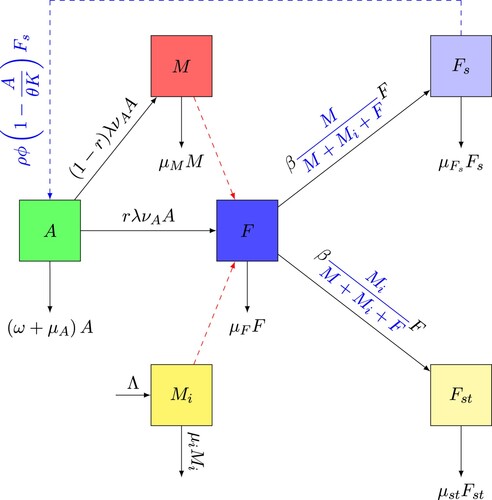
The flow of F to the compartments $F_s$ and $F_{\mathrm{st}}$ depends mainly on the number of encounters of young females not yet laying eggs with wild males and Wolbachia-infected male mosquitoes respectively, and the corresponding mating rates between them. We consider that after a release of Wolbachia-infected male mosquitoes, the total population of mosquitoes in the aerial phase can be expressed by $M+M_i+F$. The fraction $M/(M+M_i+F)$ represents the probability that a young females not yet laying eggs meets a wild male and $\mathrm{MF}/(M+M_i+F)$ is the number of encounters between wild males and young females not yet laying eggs. Thus, $\text{β}\mathrm{MF}/(M+M_i+F)$ is the number of matings between young females and wild males. Similarly, the fraction $M_i/(M+M_i+F)$ represents the probability that a young females not yet laying eggs meets a Wolbachia-infected male and $M_{i}F/(M+M_i+F)$ is the number of encounters between Wolbachia-infected male and young females not yet laying eggs. Thus, $\text{β}{M}_{i}F/(M+M_i+F)$ is the number of matings between young females and Wolbachia-infected male mosquitoes.

The mathematical equations that integrate the assumptions given above are: (10) $\{\begin{array}{l}\dot{A}\left(t\right)=\mathrm{\rho \varphi }(1-{\displaystyle \frac{A\left(t\right)}{\mathrm{\theta K}}})F_s\left(t\right)-({\nu }_A+\omega +{\mu }_A)A\left(t\right),\\ \dot{M}\left(t\right)=(1-r)\lambda {\nu }_{A}A\left(t\right)-{\mu }_{M}M\left(t\right),\\ \dot{F}=\mathrm{r\lambda }{\nu }_{A}A\left(t\right)-(\text{β}+{\mu }_F)F\left(t\right),\\ {\dot{F}}_s\left(t\right)={\displaystyle \frac{\text{β}M\left(t\right)}{M\left(t\right)+M_i\left(t\right)+F\left(t\right)}F\left(t\right)-{\mu }_{F_s}{F}_s\left(t\right)}\\ {\dot{F}}_{\mathrm{st}}\left(t\right)={\displaystyle \frac{\text{β}{M}_i\left(t\right)}{M\left(t\right)+M_i\left(t\right)+F\left(t\right)}F\left(t\right)-{\mu }_{\mathrm{st}}{F}_{\mathrm{st}}\left(t\right),}\\ {\dot{M}}_i\left(t\right)=\mathrm{\Lambda }-{\mu }_i{M}_i\left(t\right).\end{array}$(10) Since variable $F_{\mathrm{st}}$ is not present in the first four equations of system (10(10) $\{\begin{array}{l}\dot{A}\left(t\right)=\mathrm{\rho \varphi }(1-{\displaystyle \frac{A\left(t\right)}{\mathrm{\theta K}}})F_s\left(t\right)-({\nu }_A+\omega +{\mu }_A)A\left(t\right),\\ \dot{M}\left(t\right)=(1-r)\lambda {\nu }_{A}A\left(t\right)-{\mu }_{M}M\left(t\right),\\ \dot{F}=\mathrm{r\lambda }{\nu }_{A}A\left(t\right)-(\text{β}+{\mu }_F)F\left(t\right),\\ {\dot{F}}_s\left(t\right)={\displaystyle \frac{\text{β}M\left(t\right)}{M\left(t\right)+M_i\left(t\right)+F\left(t\right)}F\left(t\right)-{\mu }_{F_s}{F}_s\left(t\right)}\\ {\dot{F}}_{\mathrm{st}}\left(t\right)={\displaystyle \frac{\text{β}{M}_i\left(t\right)}{M\left(t\right)+M_i\left(t\right)+F\left(t\right)}F\left(t\right)-{\mu }_{\mathrm{st}}{F}_{\mathrm{st}}\left(t\right),}\\ {\dot{M}}_i\left(t\right)=\mathrm{\Lambda }-{\mu }_i{M}_i\left(t\right).\end{array}$(10) ), thus, according to [22] the dynamics of system (10(10) $\{\begin{array}{l}\dot{A}\left(t\right)=\mathrm{\rho \varphi }(1-{\displaystyle \frac{A\left(t\right)}{\mathrm{\theta K}}})F_s\left(t\right)-({\nu }_A+\omega +{\mu }_A)A\left(t\right),\\ \dot{M}\left(t\right)=(1-r)\lambda {\nu }_{A}A\left(t\right)-{\mu }_{M}M\left(t\right),\\ \dot{F}=\mathrm{r\lambda }{\nu }_{A}A\left(t\right)-(\text{β}+{\mu }_F)F\left(t\right),\\ {\dot{F}}_s\left(t\right)={\displaystyle \frac{\text{β}M\left(t\right)}{M\left(t\right)+M_i\left(t\right)+F\left(t\right)}F\left(t\right)-{\mu }_{F_s}{F}_s\left(t\right)}\\ {\dot{F}}_{\mathrm{st}}\left(t\right)={\displaystyle \frac{\text{β}{M}_i\left(t\right)}{M\left(t\right)+M_i\left(t\right)+F\left(t\right)}F\left(t\right)-{\mu }_{\mathrm{st}}{F}_{\mathrm{st}}\left(t\right),}\\ {\dot{M}}_i\left(t\right)=\mathrm{\Lambda }-{\mu }_i{M}_i\left(t\right).\end{array}$(10) ) is equivalent to that of the following system: (11) $\{\begin{array}{l}\dot{A}\left(t\right)=\mathrm{\rho \varphi }(1-{\displaystyle \frac{A\left(t\right)}{\mathrm{\theta K}}})F_s\left(t\right)-({\nu }_A+\omega +{\mu }_A)A\left(t\right),\\ \dot{M}\left(t\right)=(1-r)\lambda {\nu }_{A}A\left(t\right)-{\mu }_{M}M\left(t\right),\\ \dot{F}\left(t\right)=\mathrm{r\lambda }{\nu }_{A}A\left(t\right)-(\text{β}+{\mu }_F)F\left(t\right),\\ {\dot{F}}_s\left(t\right)={\displaystyle \frac{\text{β}M\left(t\right)}{M\left(t\right)+M_i\left(t\right)+F\left(t\right)}F\left(t\right)-{\mu }_{F_s}{F}_s\left(t\right),}\\ {\dot{M}}_i\left(t\right)=\mathrm{\Lambda }-{\mu }_i{M}_i\left(t\right).\end{array}$(11)

3.2. Mathematical analysis of the model

In this section, the existence, uniqueness, positivity and boundedness of the solutions are demonstrated in the same way as the results obtained in the mathematical study of system (1(1) $\{\begin{array}{l}\dot{A}\left(t\right)=\mathrm{\rho \varphi }(1-{\displaystyle \frac{A\left(t\right)}{\mathrm{\theta K}}})F_s\left(t\right)-({\nu }_A+\omega +{\mu }_A)A\left(t\right),\\ \dot{M}\left(t\right)=(1-r)\lambda {\nu }_{A}A\left(t\right)-{\mu }_{M}M\left(t\right),\\ \dot{F}\left(t\right)=\mathrm{r\lambda }{\nu }_{A}A\left(t\right)-(\text{β}+{\mu }_F)F\left(t\right),\\ {\dot{F}}_s\left(t\right)=\text{β}{\displaystyle \frac{M\left(t\right)}{M\left(t\right)+F\left(t\right)}F\left(t\right)-{\mu }_{F_s}{F}_s\left(t\right),}\end{array}$(1) ). Note that the dynamics of Wolbachia-infected males mosquitoes, i.e. the last equation of system (11(11) $\{\begin{array}{l}\dot{A}\left(t\right)=\mathrm{\rho \varphi }(1-{\displaystyle \frac{A\left(t\right)}{\mathrm{\theta K}}})F_s\left(t\right)-({\nu }_A+\omega +{\mu }_A)A\left(t\right),\\ \dot{M}\left(t\right)=(1-r)\lambda {\nu }_{A}A\left(t\right)-{\mu }_{M}M\left(t\right),\\ \dot{F}\left(t\right)=\mathrm{r\lambda }{\nu }_{A}A\left(t\right)-(\text{β}+{\mu }_F)F\left(t\right),\\ {\dot{F}}_s\left(t\right)={\displaystyle \frac{\text{β}M\left(t\right)}{M\left(t\right)+M_i\left(t\right)+F\left(t\right)}F\left(t\right)-{\mu }_{F_s}{F}_s\left(t\right),}\\ {\dot{M}}_i\left(t\right)=\mathrm{\Lambda }-{\mu }_i{M}_i\left(t\right).\end{array}$(11) ) is independent of other variables, but it can impact the dynamics of others. We can verify that its equilibrium $M_i^{\ast }=\mathrm{\Lambda }/{\mu }_i$ is locally stable, and that for any initial value $M_i\left(0\right)$, (12) $M_i\left(t\right)=M_i^{\ast }+{\mathrm{e}}^{-{\mu }_{i}t}\left(M_i\right(0)-M_i^{\ast })\to M_i^{\ast },\mathrm{as}t\to \mathrm{\infty }.$(12) Hence equilibrium $M_i^{\ast }$ is globally asymptotically stable. Moreover, we can obtain the limiting system of system (11(11) $\{\begin{array}{l}\dot{A}\left(t\right)=\mathrm{\rho \varphi }(1-{\displaystyle \frac{A\left(t\right)}{\mathrm{\theta K}}})F_s\left(t\right)-({\nu }_A+\omega +{\mu }_A)A\left(t\right),\\ \dot{M}\left(t\right)=(1-r)\lambda {\nu }_{A}A\left(t\right)-{\mu }_{M}M\left(t\right),\\ \dot{F}\left(t\right)=\mathrm{r\lambda }{\nu }_{A}A\left(t\right)-(\text{β}+{\mu }_F)F\left(t\right),\\ {\dot{F}}_s\left(t\right)={\displaystyle \frac{\text{β}M\left(t\right)}{M\left(t\right)+M_i\left(t\right)+F\left(t\right)}F\left(t\right)-{\mu }_{F_s}{F}_s\left(t\right),}\\ {\dot{M}}_i\left(t\right)=\mathrm{\Lambda }-{\mu }_i{M}_i\left(t\right).\end{array}$(11) ) as follows (13) $\{\begin{array}{l}\dot{A}\left(t\right)=\mathrm{\rho \varphi }(1-{\displaystyle \frac{A\left(t\right)}{\mathrm{\theta K}}})F_s\left(t\right)-({\nu }_A+\omega +{\mu }_A)A\left(t\right),\\ \dot{M}\left(t\right)=(1-r)\lambda {\nu }_{A}A\left(t\right)-{\mu }_{M}M\left(t\right),\\ \dot{F}\left(t\right)=\mathrm{r\lambda }{\nu }_{A}A\left(t\right)-(\text{β}+{\mu }_F)F\left(t\right),\\ {\dot{F}}_s\left(t\right)={\displaystyle \frac{\text{β}M\left(t\right)}{M\left(t\right)+M_i^{\ast }+F\left(t\right)}F\left(t\right)-{\mu }_{F_s}{F}_s\left(t\right).}\end{array}$(13) Note that, the dynamics of system (11(11) $\{\begin{array}{l}\dot{A}\left(t\right)=\mathrm{\rho \varphi }(1-{\displaystyle \frac{A\left(t\right)}{\mathrm{\theta K}}})F_s\left(t\right)-({\nu }_A+\omega +{\mu }_A)A\left(t\right),\\ \dot{M}\left(t\right)=(1-r)\lambda {\nu }_{A}A\left(t\right)-{\mu }_{M}M\left(t\right),\\ \dot{F}\left(t\right)=\mathrm{r\lambda }{\nu }_{A}A\left(t\right)-(\text{β}+{\mu }_F)F\left(t\right),\\ {\dot{F}}_s\left(t\right)={\displaystyle \frac{\text{β}M\left(t\right)}{M\left(t\right)+M_i\left(t\right)+F\left(t\right)}F\left(t\right)-{\mu }_{F_s}{F}_s\left(t\right),}\\ {\dot{M}}_i\left(t\right)=\mathrm{\Lambda }-{\mu }_i{M}_i\left(t\right).\end{array}$(11) ) is qualitatively equivalent to their limiting systems (13(13) $\{\begin{array}{l}\dot{A}\left(t\right)=\mathrm{\rho \varphi }(1-{\displaystyle \frac{A\left(t\right)}{\mathrm{\theta K}}})F_s\left(t\right)-({\nu }_A+\omega +{\mu }_A)A\left(t\right),\\ \dot{M}\left(t\right)=(1-r)\lambda {\nu }_{A}A\left(t\right)-{\mu }_{M}M\left(t\right),\\ \dot{F}\left(t\right)=\mathrm{r\lambda }{\nu }_{A}A\left(t\right)-(\text{β}+{\mu }_F)F\left(t\right),\\ {\dot{F}}_s\left(t\right)={\displaystyle \frac{\text{β}M\left(t\right)}{M\left(t\right)+M_i^{\ast }+F\left(t\right)}F\left(t\right)-{\mu }_{F_s}{F}_s\left(t\right).}\end{array}$(13) ) [19, 22, 45]. Thus, the principal results for system (11(11) $\{\begin{array}{l}\dot{A}\left(t\right)=\mathrm{\rho \varphi }(1-{\displaystyle \frac{A\left(t\right)}{\mathrm{\theta K}}})F_s\left(t\right)-({\nu }_A+\omega +{\mu }_A)A\left(t\right),\\ \dot{M}\left(t\right)=(1-r)\lambda {\nu }_{A}A\left(t\right)-{\mu }_{M}M\left(t\right),\\ \dot{F}\left(t\right)=\mathrm{r\lambda }{\nu }_{A}A\left(t\right)-(\text{β}+{\mu }_F)F\left(t\right),\\ {\dot{F}}_s\left(t\right)={\displaystyle \frac{\text{β}M\left(t\right)}{M\left(t\right)+M_i\left(t\right)+F\left(t\right)}F\left(t\right)-{\mu }_{F_s}{F}_s\left(t\right),}\\ {\dot{M}}_i\left(t\right)=\mathrm{\Lambda }-{\mu }_i{M}_i\left(t\right).\end{array}$(11) ) can be obtained by the same method as for system (13(13) $\{\begin{array}{l}\dot{A}\left(t\right)=\mathrm{\rho \varphi }(1-{\displaystyle \frac{A\left(t\right)}{\mathrm{\theta K}}})F_s\left(t\right)-({\nu }_A+\omega +{\mu }_A)A\left(t\right),\\ \dot{M}\left(t\right)=(1-r)\lambda {\nu }_{A}A\left(t\right)-{\mu }_{M}M\left(t\right),\\ \dot{F}\left(t\right)=\mathrm{r\lambda }{\nu }_{A}A\left(t\right)-(\text{β}+{\mu }_F)F\left(t\right),\\ {\dot{F}}_s\left(t\right)={\displaystyle \frac{\text{β}M\left(t\right)}{M\left(t\right)+M_i^{\ast }+F\left(t\right)}F\left(t\right)-{\mu }_{F_s}{F}_s\left(t\right).}\end{array}$(13) ).

3.2.1. The trivial equilibrium and its stability analysis

The trivial equilibrium, of system (11(11) $\{\begin{array}{l}\dot{A}\left(t\right)=\mathrm{\rho \varphi }(1-{\displaystyle \frac{A\left(t\right)}{\mathrm{\theta K}}})F_s\left(t\right)-({\nu }_A+\omega +{\mu }_A)A\left(t\right),\\ \dot{M}\left(t\right)=(1-r)\lambda {\nu }_{A}A\left(t\right)-{\mu }_{M}M\left(t\right),\\ \dot{F}\left(t\right)=\mathrm{r\lambda }{\nu }_{A}A\left(t\right)-(\text{β}+{\mu }_F)F\left(t\right),\\ {\dot{F}}_s\left(t\right)={\displaystyle \frac{\text{β}M\left(t\right)}{M\left(t\right)+M_i\left(t\right)+F\left(t\right)}F\left(t\right)-{\mu }_{F_s}{F}_s\left(t\right),}\\ {\dot{M}}_i\left(t\right)=\mathrm{\Lambda }-{\mu }_i{M}_i\left(t\right).\end{array}$(11) ) is obtained by setting the right-hand sides of the equations in system (11(11) $\{\begin{array}{l}\dot{A}\left(t\right)=\mathrm{\rho \varphi }(1-{\displaystyle \frac{A\left(t\right)}{\mathrm{\theta K}}})F_s\left(t\right)-({\nu }_A+\omega +{\mu }_A)A\left(t\right),\\ \dot{M}\left(t\right)=(1-r)\lambda {\nu }_{A}A\left(t\right)-{\mu }_{M}M\left(t\right),\\ \dot{F}\left(t\right)=\mathrm{r\lambda }{\nu }_{A}A\left(t\right)-(\text{β}+{\mu }_F)F\left(t\right),\\ {\dot{F}}_s\left(t\right)={\displaystyle \frac{\text{β}M\left(t\right)}{M\left(t\right)+M_i\left(t\right)+F\left(t\right)}F\left(t\right)-{\mu }_{F_s}{F}_s\left(t\right),}\\ {\dot{M}}_i\left(t\right)=\mathrm{\Lambda }-{\mu }_i{M}_i\left(t\right).\end{array}$(11) ) to zero. This is given by: ${\mathcal{E}}_2=(A^{\ast },M^{\ast },F^{\ast },F_s^{\ast },M_i^{\ast })=(0,0,0,0,M_i^{\ast }),$corresponding to the state where wild mosquitoes are absent and there is only a constant population of Wolbachia-infected males.

Now, we analyse the stability conditions of the trivial equilibrium point. To do this, we calculate the Jacobian matrix of system (11(11) $\{\begin{array}{l}\dot{A}\left(t\right)=\mathrm{\rho \varphi }(1-{\displaystyle \frac{A\left(t\right)}{\mathrm{\theta K}}})F_s\left(t\right)-({\nu }_A+\omega +{\mu }_A)A\left(t\right),\\ \dot{M}\left(t\right)=(1-r)\lambda {\nu }_{A}A\left(t\right)-{\mu }_{M}M\left(t\right),\\ \dot{F}\left(t\right)=\mathrm{r\lambda }{\nu }_{A}A\left(t\right)-(\text{β}+{\mu }_F)F\left(t\right),\\ {\dot{F}}_s\left(t\right)={\displaystyle \frac{\text{β}M\left(t\right)}{M\left(t\right)+M_i\left(t\right)+F\left(t\right)}F\left(t\right)-{\mu }_{F_s}{F}_s\left(t\right),}\\ {\dot{M}}_i\left(t\right)=\mathrm{\Lambda }-{\mu }_i{M}_i\left(t\right).\end{array}$(11) ), given by $J=\left(\begin{array}{ccccc}-(\mathrm{\rho \varphi }\frac{F_s}{\mathrm{\theta K}}+{\nu }_A)& 0& 0& \mathrm{\rho \varphi }(1-\frac{A}{\mathrm{\theta K}})& 0\\ (1-r)\lambda {\nu }_A& -{\mu }_M& 0& 0& 0\\ \mathrm{r\lambda }{\nu }_A& 0& -(\text{β}+{\mu }_F)& 0& 0\\ 0& \frac{\text{β}F(F+M_i)}{(M+M_i+F{)}^2}& \frac{\text{β}M(M+M_i)}{(M+M_i+F{)}^2}& -{\mu }_{F_s}& -\frac{\text{β}\mathrm{MF}}{(M+M_i+F{)}^2}\\ 0& 0& 0& 0& -{\mu }_i\end{array}\right)$

Theorem 3.1

The trivial equilibrium of system (11(11) $\{\begin{array}{l}\dot{A}\left(t\right)=\mathrm{\rho \varphi }(1-{\displaystyle \frac{A\left(t\right)}{\mathrm{\theta K}}})F_s\left(t\right)-({\nu }_A+\omega +{\mu }_A)A\left(t\right),\\ \dot{M}\left(t\right)=(1-r)\lambda {\nu }_{A}A\left(t\right)-{\mu }_{M}M\left(t\right),\\ \dot{F}\left(t\right)=\mathrm{r\lambda }{\nu }_{A}A\left(t\right)-(\text{β}+{\mu }_F)F\left(t\right),\\ {\dot{F}}_s\left(t\right)={\displaystyle \frac{\text{β}M\left(t\right)}{M\left(t\right)+M_i\left(t\right)+F\left(t\right)}F\left(t\right)-{\mu }_{F_s}{F}_s\left(t\right),}\\ {\dot{M}}_i\left(t\right)=\mathrm{\Lambda }-{\mu }_i{M}_i\left(t\right).\end{array}$(11) ), given by ${\mathcal{E}}_2=(0,0,0,0,M_i^{\ast })$, is locally asymptotically stable.

Proof.

The Jacobian matrix of system (11(11) $\{\begin{array}{l}\dot{A}\left(t\right)=\mathrm{\rho \varphi }(1-{\displaystyle \frac{A\left(t\right)}{\mathrm{\theta K}}})F_s\left(t\right)-({\nu }_A+\omega +{\mu }_A)A\left(t\right),\\ \dot{M}\left(t\right)=(1-r)\lambda {\nu }_{A}A\left(t\right)-{\mu }_{M}M\left(t\right),\\ \dot{F}\left(t\right)=\mathrm{r\lambda }{\nu }_{A}A\left(t\right)-(\text{β}+{\mu }_F)F\left(t\right),\\ {\dot{F}}_s\left(t\right)={\displaystyle \frac{\text{β}M\left(t\right)}{M\left(t\right)+M_i\left(t\right)+F\left(t\right)}F\left(t\right)-{\mu }_{F_s}{F}_s\left(t\right),}\\ {\dot{M}}_i\left(t\right)=\mathrm{\Lambda }-{\mu }_i{M}_i\left(t\right).\end{array}$(11) ) at the trivial equilibrium point ${\mathcal{E}}_2$ has the following form $J_{{\mathcal{E}}_2}=\left(\begin{array}{ccccc}-({\nu }_A+\omega +{\mu }_A)& 0& 0& \mathrm{\rho \varphi }& 0\\ (1-r)\lambda {\nu }_A& -{\mu }_M& 0& 0& 0\\ \mathrm{r\lambda }{\nu }_A& 0& -(\text{β}+{\mu }_F)& 0& 0\\ 0& 0& 0& -{\mu }_{F_s}& 0\\ 0& 0& 0& 0& -{\mu }_i\end{array}\right)$The eigenvalues of $J_{{\mathcal{E}}_2}$ at the equilibrium point ${\mathcal{E}}_2=(0,0,0,0,M_i^{\ast })$ are $-({\nu }_A+\omega +{\mu }_A)$, $-{\mu }_M$, $-(\text{β}+{\mu }_F)$, $-{\mu }_{F_s}$ and $-{\mu }_i$ which are all negative, therefore ${\mathcal{E}}_2$ is always locally asymptotically stable.

Theorem 3.2

The trivial equilibrium of system (11(11) $\{\begin{array}{l}\dot{A}\left(t\right)=\mathrm{\rho \varphi }(1-{\displaystyle \frac{A\left(t\right)}{\mathrm{\theta K}}})F_s\left(t\right)-({\nu }_A+\omega +{\mu }_A)A\left(t\right),\\ \dot{M}\left(t\right)=(1-r)\lambda {\nu }_{A}A\left(t\right)-{\mu }_{M}M\left(t\right),\\ \dot{F}\left(t\right)=\mathrm{r\lambda }{\nu }_{A}A\left(t\right)-(\text{β}+{\mu }_F)F\left(t\right),\\ {\dot{F}}_s\left(t\right)={\displaystyle \frac{\text{β}M\left(t\right)}{M\left(t\right)+M_i\left(t\right)+F\left(t\right)}F\left(t\right)-{\mu }_{F_s}{F}_s\left(t\right),}\\ {\dot{M}}_i\left(t\right)=\mathrm{\Lambda }-{\mu }_i{M}_i\left(t\right).\end{array}$(11) ), given by ${\mathcal{E}}_2$, is globally asymptotically stable whenever $\mathcal{N}\le 1$ and unstable if $\mathcal{N}>1$.

Proof.

Consider the Lyapunov function for system (11(11) $\{\begin{array}{l}\dot{A}\left(t\right)=\mathrm{\rho \varphi }(1-{\displaystyle \frac{A\left(t\right)}{\mathrm{\theta K}}})F_s\left(t\right)-({\nu }_A+\omega +{\mu }_A)A\left(t\right),\\ \dot{M}\left(t\right)=(1-r)\lambda {\nu }_{A}A\left(t\right)-{\mu }_{M}M\left(t\right),\\ \dot{F}\left(t\right)=\mathrm{r\lambda }{\nu }_{A}A\left(t\right)-(\text{β}+{\mu }_F)F\left(t\right),\\ {\dot{F}}_s\left(t\right)={\displaystyle \frac{\text{β}M\left(t\right)}{M\left(t\right)+M_i\left(t\right)+F\left(t\right)}F\left(t\right)-{\mu }_{F_s}{F}_s\left(t\right),}\\ {\dot{M}}_i\left(t\right)=\mathrm{\Lambda }-{\mu }_i{M}_i\left(t\right).\end{array}$(11) ): (14) $\mathcal{V}=\frac{{\mu }_{F_s}[(1-r)(\text{β}+{\mu }_F)+r{\mu }_M]}{(1-r)\mathrm{r\rho \varphi }\text{β}}A+M+F+\frac{(1-r)(\text{β}+{\mu }_F)+r{\mu }_M}{(1-r)r\text{β}}{F}_s$(14) with Lyapunov derivative given by $\begin{array}{rl}\dot{\mathcal{V}}& =\frac{{\mu }_{F_s}[(1-r)(\text{β}+{\mu }_F)+r{\mu }_M]}{(1-r)\mathrm{r\rho \varphi }\text{β}}\dot{A}+\dot{M}+\dot{F}+\frac{(1-r)(\text{β}+{\mu }_F)+r{\mu }_M}{(1-r)r\text{β}}\dot{F_s}\\ & =\frac{{\mu }_{F_s}[(1-r)(\text{β}+{\mu }_F)+r{\mu }_M]}{(1-r)\mathrm{r\rho \varphi }\text{β}}[\mathrm{\rho \varphi }(1-\frac{A}{\mathrm{\theta K}})F_s-({\nu }_A+\omega +{\mu }_A)A]\\ & +\left[\right(1-r)\lambda {\nu }_{A}A-{\mu }_{M}M]+[\mathrm{r\lambda }{\nu }_{A}A-(\text{β}+{\mu }_F)F]\\ & +\frac{(1-r)(\text{β}+{\mu }_F)+r{\mu }_M}{(1-r)r\text{β}}[\frac{\text{β}M}{M+M_i+F}F-{\mu }_{F_s}{F}_s]\\ & =[\lambda {\nu }_A-\frac{{\mu }_{F_s}[(1-r)(\text{β}+{\mu }_F)+r{\mu }_M]({\nu }_A+\omega +{\mu }_A)}{(1-r)\mathrm{r\rho \varphi }\text{β}}]A\\ & -{\mu }_{M}M+\frac{(1-r)(\text{β}+{\mu }_F)+r{\mu }_M}{(1-r)r}\frac{M}{M+M_i+F}F-(\text{β}+{\mu }_F)F\\ & -\frac{{\mu }_{F_s}[(1-r)(\text{β}+{\mu }_F)+r{\mu }_M]}{(1-r)\mathrm{r\rho \varphi }\text{β}}\frac{A{F}_s}{\mathrm{\theta K}}.\end{array}$Then, using the fact that there exists a $ϵ\in ]0,1]$ such that $\frac{M}{M+M_i+F}\le ϵ$, and taking $ϵ=\frac{(1-r)r(\text{β}+{\mu }_F)}{(1-r)(\text{β}+{\mu }_F)+r{\mu }_M}$, we have the following inequality: $\begin{array}{rl}\dot{\mathcal{V}}& \le [\lambda {\nu }_A-\frac{{\mu }_{F_s}[(1-r)(\text{β}+{\mu }_F)+r{\mu }_M]({\nu }_A+\omega +{\mu }_A)}{(1-r)\mathrm{r\rho \varphi }\text{β}}]A\\ & -\frac{{\mu }_{F_s}[(1-r)(\text{β}+{\mu }_F)+r{\mu }_M]}{(1-r)\mathrm{r\rho \varphi }\text{β}}\frac{A{F}_s}{\mathrm{\theta K}}-{\mu }_{M}M\\ & \le \frac{(1-r)\mathrm{r\rho \varphi }\text{β}}{{\mu }_{F_s}[(1-r)(\text{β}+{\mu }_F)+r{\mu }_M]({\nu }_A+\omega +{\mu }_A)}(\mathcal{N}-1)A\\ & -\frac{{\mu }_{F_s}[(1-r)(\text{β}+{\mu }_F)+r{\mu }_M]}{(1-r)\mathrm{r\rho \varphi }\text{β}}\frac{A{F}_s}{\mathrm{\theta K}}-{\mu }_{M}M\\ & \le \frac{(1-r)\mathrm{r\rho \varphi }\text{β}}{{\mu }_{F_s}[(1-r)(\text{β}+{\mu }_F)+r{\mu }_M]({\nu }_A+\omega +{\mu }_A)}(\mathcal{N}-1)A.\end{array}$Since all the model parameters are non-negative, it follows that $\dot{\mathcal{V}}\le 0$ for $\mathcal{N}\le 1$. The largest compact invariant set in $\left\{\right(A,M,F,F_s,M_i)\in {\mathbb{R}}_{+}^5:\dot{\mathcal{V}}=0\}$ is the singleton $\left\{{\mathcal{E}}_2\right\}$. It follows from the LaSalle Invariance Principle [19, 46, 47] that every solution of system (11(11) $\{\begin{array}{l}\dot{A}\left(t\right)=\mathrm{\rho \varphi }(1-{\displaystyle \frac{A\left(t\right)}{\mathrm{\theta K}}})F_s\left(t\right)-({\nu }_A+\omega +{\mu }_A)A\left(t\right),\\ \dot{M}\left(t\right)=(1-r)\lambda {\nu }_{A}A\left(t\right)-{\mu }_{M}M\left(t\right),\\ \dot{F}\left(t\right)=\mathrm{r\lambda }{\nu }_{A}A\left(t\right)-(\text{β}+{\mu }_F)F\left(t\right),\\ {\dot{F}}_s\left(t\right)={\displaystyle \frac{\text{β}M\left(t\right)}{M\left(t\right)+M_i\left(t\right)+F\left(t\right)}F\left(t\right)-{\mu }_{F_s}{F}_s\left(t\right),}\\ {\dot{M}}_i\left(t\right)=\mathrm{\Lambda }-{\mu }_i{M}_i\left(t\right).\end{array}$(11) ) with initial conditions in ${\mathbb{R}}_{+}^5$ converge to the trivial equilibrium ${\mathcal{E}}_2$ as $t\to \mathrm{\infty }$. Thus $(A,M,F,F_s,M_i)\to (0,0,0,0,M_i^{\ast })$ when $t\to \mathrm{\infty }$ for $\mathcal{N}\le 1$. So, From the LaSalle principle we deduce the attractiveness of ${\mathcal{E}}_2$. Since ${\mathcal{E}}_2$ is locally asymptotically stable when $\mathcal{N}\le 1$, we deduce that it is not only attractive, but it is also globally asymptotically stable. This ends the proof.

3.2.2. The non-trivial equilibrium and its stability analysis

3.2.2.1 Existence of non-trivial equilibrium

In this subsection, we consider that the basic offspring number $\mathcal{N}$ is greater than unity. By setting the right-hand sides of the equations of system (11(11) $\{\begin{array}{l}\dot{A}\left(t\right)=\mathrm{\rho \varphi }(1-{\displaystyle \frac{A\left(t\right)}{\mathrm{\theta K}}})F_s\left(t\right)-({\nu }_A+\omega +{\mu }_A)A\left(t\right),\\ \dot{M}\left(t\right)=(1-r)\lambda {\nu }_{A}A\left(t\right)-{\mu }_{M}M\left(t\right),\\ \dot{F}\left(t\right)=\mathrm{r\lambda }{\nu }_{A}A\left(t\right)-(\text{β}+{\mu }_F)F\left(t\right),\\ {\dot{F}}_s\left(t\right)={\displaystyle \frac{\text{β}M\left(t\right)}{M\left(t\right)+M_i\left(t\right)+F\left(t\right)}F\left(t\right)-{\mu }_{F_s}{F}_s\left(t\right),}\\ {\dot{M}}_i\left(t\right)=\mathrm{\Lambda }-{\mu }_i{M}_i\left(t\right).\end{array}$(11) ) to zero and expressing the variables in terms of M, we obtain the non-trivial equilibrium. Thus, the non-trivial equilibrium point ${\mathcal{E}}_3=(A^{\ast \ast },M^{\ast \ast },F^{\ast \ast },F_s^{\ast \ast },M_i^{\ast })$ satisfy the following relations: $\{\begin{array}{l}{A}^{\ast \ast }={\displaystyle \frac{{\mu }_M{M}^{\ast \ast }}{(1-r)\lambda {\nu }_A},}\\ F^{\ast \ast }={\displaystyle \frac{r{\mu }_M{M}^{\ast \ast }}{(1-r)(\text{β}+{\mu }_F)},}\\ F_s^{\ast \ast }={\displaystyle \frac{r{\mu }_M\text{β}{\left(M^{\ast \ast }\right)}^2}{{\mu }_{F_s}[\left(\right(1-r)(\text{β}+{\mu }_F)+r{\mu }_M)M^{\ast \ast }+(1-r\left)(\text{β}+{\mu }_F)M_i^{\ast }\right]},}\end{array}$where $M^{\ast \ast }$ is a solution of the second degree equation (15) $g\left(M^{\ast \ast }\right)=a_1{\left(M^{\ast \ast }\right)}^2+a_2{M}^{\ast \ast }+a_3=0,$(15) with coefficients $\begin{array}{rl}{a}_1& =\frac{r{\mu }_M\text{β}\mathrm{\rho \varphi }}{{\mu }_{F_s}\mathrm{\theta K}({\nu }_A+\omega +{\mu }_A)((1-r)(\text{β}+{\mu }_F)+r{\mu }_M)},\\ a_2& =1-\frac{(1-r)\mathrm{r\lambda }{\nu }_A\text{β}\mathrm{\rho \varphi }}{{\mu }_{F_s}({\nu }_A+\omega +{\mu }_A)\left[\right(1-r\left)\right(\text{β}+{\mu }_F)+r{\mu }_M]}=1-\mathcal{N},\\ a_3& =\frac{(1-r)(\text{β}+{\mu }_F)M_i^{\ast }}{((1-r)(\text{β}+{\mu }_F)+r{\mu }_M)}.\end{array}$It should be noted that the coefficients $a_1$ and $a_3$ of the quadratic Equation (15(15) $g\left(M^{\ast \ast }\right)=a_1{\left(M^{\ast \ast }\right)}^2+a_2{M}^{\ast \ast }+a_3=0,$(15) ) are always positive, however the coefficient $a_2$ is negative if the basic offspring number $\mathcal{N}$ is greater than unity. It follows that $g\left(M^{\ast \ast }\right)$ has two or no positive roots if and only if $\mathcal{N}>1$ and $a_2^2-4a_1{a}_3>0$ or $\mathcal{N}>1$ and $a_2^2-4a_1{a}_3<0$, respectively. Then, the conditions for biological existence of the non-trivial equilibrium points become (16) $\mathcal{N}>1\mathrm{and}{M}_i^{\ast }<\frac{r{\lambda }^2{\nu }_A^2\text{β}\mathrm{\rho \varphi \theta K}(1-r)}{4{\mu }_M{\mu }_{F_s}({\nu }_A+\omega +{\mu }_A)(\text{β}+{\mu }_F)}{(1-\frac{1}{\mathcal{N}})}^2.$(16) Let $M_i^{\mathrm{crit}}=\frac{r{\lambda }^2{\nu }_A^2\text{β}\mathrm{\rho \varphi \theta K}(1-r){(1-\frac{1}{\mathcal{N}})}^2}{4{\mu }_M{\mu }_{F_s}({\nu }_A+\omega +{\mu }_A)(\text{β}+{\mu }_F)}.$Then, we have $\frac{{(\mathcal{N}-1)}^2}{M_i^{\mathrm{crit}}}=\frac{4{\mu }_M{\mu }_{F_s}({\nu }_A+\omega +{\mu }_A)(\text{β}+{\mu }_F){\mathcal{N}}^2}{r{\lambda }^2{\nu }_A^2\text{β}\mathrm{\rho \varphi \theta K}(1-r)}.$So condition (16(16) $\mathcal{N}>1\mathrm{and}{M}_i^{\ast }<\frac{r{\lambda }^2{\nu }_A^2\text{β}\mathrm{\rho \varphi \theta K}(1-r)}{4{\mu }_M{\mu }_{F_s}({\nu }_A+\omega +{\mu }_A)(\text{β}+{\mu }_F)}{(1-\frac{1}{\mathcal{N}})}^2.$(16) ) becomes: $\mathcal{N}>1$ and $M_i^{\ast }<M_i^{\mathrm{crit}}$ . Thus, the solutions are given by $\begin{array}{rl}{M}_{-}^{\ast \ast }& =\frac{\lambda {\nu }_A\mathrm{\theta K}(1-r)(\mathcal{N}-1)}{2{\mu }_M\mathcal{N}}[1-{\displaystyle \sqrt{1-\frac{M_i^{\ast }}{M_i^{\mathrm{crit}}}}}],\mathrm{and}\\ M_{+}^{\ast \ast }& =\frac{\lambda {\nu }_A\mathrm{\theta K}(1-r)(\mathcal{N}-1)}{2{\mu }_M\mathcal{N}}[1+{\displaystyle \sqrt{1-\frac{M_i^{\ast }}{M_i^{\mathrm{crit}}}}}].\end{array}$Moreover, under conditions (16(16) $\mathcal{N}>1\mathrm{and}{M}_i^{\ast }<\frac{r{\lambda }^2{\nu }_A^2\text{β}\mathrm{\rho \varphi \theta K}(1-r)}{4{\mu }_M{\mu }_{F_s}({\nu }_A+\omega +{\mu }_A)(\text{β}+{\mu }_F)}{(1-\frac{1}{\mathcal{N}})}^2.$(16) ), we have $\mathcal{N}-1>0\mathrm{and}\frac{M_i^{\ast }}{M_i^{\mathrm{crit}}}<1,\mathrm{thus}{M}_{-}^{\ast \ast }>0\mathrm{and}{M}_{+}^{\ast \ast }>0.$Therefore, under conditions (16(16) $\mathcal{N}>1\mathrm{and}{M}_i^{\ast }<\frac{r{\lambda }^2{\nu }_A^2\text{β}\mathrm{\rho \varphi \theta K}(1-r)}{4{\mu }_M{\mu }_{F_s}({\nu }_A+\omega +{\mu }_A)(\text{β}+{\mu }_F)}{(1-\frac{1}{\mathcal{N}})}^2.$(16) ), system (11(11) $\{\begin{array}{l}\dot{A}\left(t\right)=\mathrm{\rho \varphi }(1-{\displaystyle \frac{A\left(t\right)}{\mathrm{\theta K}}})F_s\left(t\right)-({\nu }_A+\omega +{\mu }_A)A\left(t\right),\\ \dot{M}\left(t\right)=(1-r)\lambda {\nu }_{A}A\left(t\right)-{\mu }_{M}M\left(t\right),\\ \dot{F}\left(t\right)=\mathrm{r\lambda }{\nu }_{A}A\left(t\right)-(\text{β}+{\mu }_F)F\left(t\right),\\ {\dot{F}}_s\left(t\right)={\displaystyle \frac{\text{β}M\left(t\right)}{M\left(t\right)+M_i\left(t\right)+F\left(t\right)}F\left(t\right)-{\mu }_{F_s}{F}_s\left(t\right),}\\ {\dot{M}}_i\left(t\right)=\mathrm{\Lambda }-{\mu }_i{M}_i\left(t\right).\end{array}$(11) ) has two positive equilibria ${\mathcal{E}}_3^{-}$ and ${\mathcal{E}}_3^{+}$, corresponding to $M_{-}^{\ast \ast }$ and $M_{+}^{\ast \ast }$.

Thus, the following result have been established:

Theorem 3.3

Assume that $\mathcal{N}>1$.

(i)

If $M_i^{\ast }>M_i^{\mathrm{crit}}$ , then system (11(11) $\{\begin{array}{l}\dot{A}\left(t\right)=\mathrm{\rho \varphi }(1-{\displaystyle \frac{A\left(t\right)}{\mathrm{\theta K}}})F_s\left(t\right)-({\nu }_A+\omega +{\mu }_A)A\left(t\right),\\ \dot{M}\left(t\right)=(1-r)\lambda {\nu }_{A}A\left(t\right)-{\mu }_{M}M\left(t\right),\\ \dot{F}\left(t\right)=\mathrm{r\lambda }{\nu }_{A}A\left(t\right)-(\text{β}+{\mu }_F)F\left(t\right),\\ {\dot{F}}_s\left(t\right)={\displaystyle \frac{\text{β}M\left(t\right)}{M\left(t\right)+M_i\left(t\right)+F\left(t\right)}F\left(t\right)-{\mu }_{F_s}{F}_s\left(t\right),}\\ {\dot{M}}_i\left(t\right)=\mathrm{\Lambda }-{\mu }_i{M}_i\left(t\right).\end{array}$(11) ) has no positive equilibrium point.

(ii)

If $M_i^{\ast }<M_i^{\mathrm{crit}}$ , then system (11(11) $\{\begin{array}{l}\dot{A}\left(t\right)=\mathrm{\rho \varphi }(1-{\displaystyle \frac{A\left(t\right)}{\mathrm{\theta K}}})F_s\left(t\right)-({\nu }_A+\omega +{\mu }_A)A\left(t\right),\\ \dot{M}\left(t\right)=(1-r)\lambda {\nu }_{A}A\left(t\right)-{\mu }_{M}M\left(t\right),\\ \dot{F}\left(t\right)=\mathrm{r\lambda }{\nu }_{A}A\left(t\right)-(\text{β}+{\mu }_F)F\left(t\right),\\ {\dot{F}}_s\left(t\right)={\displaystyle \frac{\text{β}M\left(t\right)}{M\left(t\right)+M_i\left(t\right)+F\left(t\right)}F\left(t\right)-{\mu }_{F_s}{F}_s\left(t\right),}\\ {\dot{M}}_i\left(t\right)=\mathrm{\Lambda }-{\mu }_i{M}_i\left(t\right).\end{array}$(11) ) admits two positive equilibria points ${\mathcal{E}}_3^{\pm }=(A_{\pm }^{\ast \ast },M_{\pm }^{\ast \ast },F_{\pm }^{\ast \ast },F_{s\pm }^{\ast \ast },M_i^{\ast })$where $\{\begin{array}{l}{A}_{\pm }^{\ast \ast }={\displaystyle \frac{{\mu }_M{M}_{\pm }^{\ast \ast }}{(1-r)\lambda {\nu }_A},}\\ M_{\pm }^{\ast \ast }={\displaystyle \frac{{\nu }_A\mathrm{\theta K}(1-r)\lambda }{2{\mu }_M\mathcal{N}}}\\ \times \left(\right(\mathcal{N}-1)\pm {\displaystyle \sqrt{{\displaystyle \frac{4{\mu }_M{\mu }_{F_s}({\nu }_A+\omega +{\mu }_A)(\text{β}+{\mu }_F){\mathcal{N}}^2(M_i^{\mathrm{crit}}-M_i^{\ast })}{r{\lambda }^2{\nu }_A^2\text{β}\mathrm{\rho \varphi \theta K}(1-r)}}}}),\\ F_{\pm }^{\ast \ast }={\displaystyle \frac{r{\mu }_M{M}_{\pm }^{\ast \ast }}{(1-r)(\text{β}+{\mu }_F)},}\\ F_{s\pm }^{\ast \ast }={\displaystyle \frac{r{\mu }_M\text{β}{\left(M_{\pm }^{\ast \ast }\right)}^2}{{\mu }_{F_s}[\left(\right(1-r)(\text{β}+{\mu }_F)+r{\mu }_M)M_{\pm }^{\ast \ast }+(1-r\left)(\text{β}+{\mu }_F)M_i^{\ast }\right]}.}\end{array}$

Remark 3.1

Notice that if $M_i^{\ast }=M_i^{\mathrm{crit}}$ , then ${\mathcal{E}}_3^{-}$ and ${\mathcal{E}}_3^{+}$ collapse to an equilibrium ${\mathcal{E}}_3$ with $M^{\ast \ast }=\frac{\mathrm{\theta K}{\nu }_A\lambda (1-r)({\mathcal{N}}^{\ast }-1)}{2{\mu }_M{\mathcal{N}}^{\ast }},$which provides the minimum threshold condition ${\mathcal{N}}^{\ast }=1+\frac{\begin{array}{l}2(1-r)(\text{β}+{\mu }_F)M_i^{\ast }\\ +{\displaystyle \sqrt{(1-r)(\text{β}+{\mu }_F)M_i^{\ast }\left[\right(1-r\left)\right(\text{β}+{\mu }_F\left)\right(1+M_i^{\ast })+r{\mu }_M]}}\end{array}}{(1-r)(\text{β}+{\mu }_F)+r{\mu }_M}$for the existence of the non-trivial equilibria, with ${\mathcal{N}}^{\ast }>1$.

Remark 3.2

According to Theorem 3.3, the constant release system (11(11) $\{\begin{array}{l}\dot{A}\left(t\right)=\mathrm{\rho \varphi }(1-{\displaystyle \frac{A\left(t\right)}{\mathrm{\theta K}}})F_s\left(t\right)-({\nu }_A+\omega +{\mu }_A)A\left(t\right),\\ \dot{M}\left(t\right)=(1-r)\lambda {\nu }_{A}A\left(t\right)-{\mu }_{M}M\left(t\right),\\ \dot{F}\left(t\right)=\mathrm{r\lambda }{\nu }_{A}A\left(t\right)-(\text{β}+{\mu }_F)F\left(t\right),\\ {\dot{F}}_s\left(t\right)={\displaystyle \frac{\text{β}M\left(t\right)}{M\left(t\right)+M_i\left(t\right)+F\left(t\right)}F\left(t\right)-{\mu }_{F_s}{F}_s\left(t\right),}\\ {\dot{M}}_i\left(t\right)=\mathrm{\Lambda }-{\mu }_i{M}_i\left(t\right).\end{array}$(11) ) has a threshold $M_i^{\mathrm{crit}}$ for the release amount $M_i^{\ast }$. When the release amount $M_i^{\ast }>M_i^{\mathrm{crit}}$ thus this leads to an elimination of the population of wild mosquitoes.

3.2.2.2 Stability of the non-trivial equilibria

In this subsection, we assume that $\mathcal{N}>1$ and $M_i^{\ast }<M_i^{\mathrm{crit}}$ . Thus, we will analyse the stability of the equilibria ${\mathcal{E}}_3^{-}$ and ${\mathcal{E}}_3^{+}$. For these points it is clear that $-{\mu }_i$ is an eigenvalue of the Jacobian $J_{{\mathcal{E}}_3}$. To determine the characteristic equation for the other four eigenvalues, we use the following equations obtained at equilibrium of system (11(11) $\{\begin{array}{l}\dot{A}\left(t\right)=\mathrm{\rho \varphi }(1-{\displaystyle \frac{A\left(t\right)}{\mathrm{\theta K}}})F_s\left(t\right)-({\nu }_A+\omega +{\mu }_A)A\left(t\right),\\ \dot{M}\left(t\right)=(1-r)\lambda {\nu }_{A}A\left(t\right)-{\mu }_{M}M\left(t\right),\\ \dot{F}\left(t\right)=\mathrm{r\lambda }{\nu }_{A}A\left(t\right)-(\text{β}+{\mu }_F)F\left(t\right),\\ {\dot{F}}_s\left(t\right)={\displaystyle \frac{\text{β}M\left(t\right)}{M\left(t\right)+M_i\left(t\right)+F\left(t\right)}F\left(t\right)-{\mu }_{F_s}{F}_s\left(t\right),}\\ {\dot{M}}_i\left(t\right)=\mathrm{\Lambda }-{\mu }_i{M}_i\left(t\right).\end{array}$(11) ). $\begin{array}{rl}& \mathrm{\rho \varphi }\frac{F_s^{\ast \ast }}{\mathrm{\theta K}}+{\nu }_A+\omega +{\mu }_A=\frac{\mathrm{\rho \varphi }\text{β}{M}^{\ast \ast }{F}^{\ast \ast }}{{\mu }_{F_s}\mathrm{\theta K}(M^{\ast \ast }+M_i^{\ast }+F^{\ast \ast })}+{\nu }_A+\omega +{\mu }_A,\\ & \mathrm{\rho \varphi }(1-\frac{A^{\ast \ast }}{\mathrm{\theta K}})=\frac{{\mu }_{F_s}({\nu }_A+\omega +{\mu }_A)(M^{\ast \ast }+M_i^{\ast }+F^{\ast \ast })A^{\ast \ast }}{\text{β}{M}^{\ast \ast }{F}^{\ast \ast }},\\ & \mathrm{r\lambda }{\nu }_A\mathrm{\rho \varphi }(1-\frac{A^{\ast \ast }}{\mathrm{\theta K}})\frac{\text{β}{M}^{\ast \ast }(M^{\ast \ast }+M_i^{\ast })}{{(M^{\ast \ast }+M_i^{\ast }+F^{\ast \ast })}^2}=\frac{{\mu }_{F_s}(\text{β}+{\mu }_F)({\nu }_A+\omega +{\mu }_A)(M^{\ast \ast }+M_i^{\ast })}{M^{\ast \ast }+M_i^{\ast }+F^{\ast \ast }},\\ & {\nu }_A\mathrm{\rho \varphi \lambda }(1-r)(1-\frac{A^{\ast \ast }}{\mathrm{\theta K}})\frac{\text{β}{F}^{\ast \ast }(F^{\ast \ast }+M_i^{\ast })}{{(M^{\ast \ast }+M_i^{\ast }+F^{\ast \ast })}^2}=\frac{{\mu }_{F_s}{\mu }_M({\nu }_A+\omega +{\mu }_A)(F^{\ast \ast }+M_i^{\ast })}{M^{\ast \ast }+M_i^{\ast }+F^{\ast \ast }}.\end{array}$After some manipulation it can be seen that the eigenvalues are the roots of the polynomial (17) $Q\left(x\right)=x^4+b_1{x}^3+b_2{x}^2+b_{3}x+b_4,$(17) with $\begin{array}{rl}{b}_1& =\frac{\mathrm{\rho \varphi }\text{β}{M}^{\ast \ast }{F}^{\ast \ast }}{{\mu }_{F_s}\mathrm{\theta K}(M^{\ast \ast }+M_i^{\ast }+F^{\ast \ast })}+{\nu }_A+\omega +{\mu }_A+{\mu }_M+{\mu }_F+{\mu }_{F_s}+\text{β},\\ b_2& =({\mu }_M+{\mu }_F+{\mu }_{F_s}+\text{β})[\frac{\mathrm{\rho \varphi }\text{β}{M}^{\ast \ast }{F}^{\ast \ast }}{{\mu }_{F_s}\mathrm{\theta K}(M^{\ast \ast }+M_i^{\ast }+F^{\ast \ast })}+{\nu }_A+\omega +{\mu }_A]\\ & +{\mu }_M({\mu }_F+{\mu }_{F_s}+\text{β}),\\ b_3& =\frac{\mathrm{\rho \varphi }\text{β}(({\mu }_M+{\mu }_{F_s})(\text{β}+{\mu }_F)+{\mu }_M{\mu }_{F_s})}{{\mu }_{F_s}\mathrm{\theta K}(M^{\ast \ast }+M_i^{\ast }+F^{\ast \ast })}+{\mu }_M(\text{β}+{\mu }_F)({\mu }_M+{\nu }_A+\omega +{\mu }_A)\\ & +\frac{{\mu }_M{\mu }_{F_s}({\nu }_A+\omega +{\mu }_A)({\mu }_M{M}^{\ast \ast }+(\text{β}+{\mu }_F)F^{\ast \ast })}{M^{\ast \ast }+M_i^{\ast }+F^{\ast \ast }},\\ b_4& =\frac{r{\mu }_M^2\mathrm{\rho \varphi }\text{β}({\left(M^{\ast \ast }\right)}^2-\frac{{\mu }_{F_s}\mathrm{\theta K}(1-r)({\nu }_A+\omega +{\mu }_A)(\text{β}+{\mu }_F)M_i^{\ast }}{r{\mu }_M\mathrm{\rho \varphi }\text{β}})}{\mathrm{\theta K}(1-r)(M^{\ast \ast }+M_i^{\ast }+F^{\ast \ast })}.\end{array}$By the Routh-Hurwitz criteria, the roots of a polynomial of order four have negative real parts if and only if $b_i>0$, with $i=1,\dots ,4$ and $(b_1{b}_2-b_3)b_3>b_1^2{b}_4$. It is clear that for the polynomial (17(17) $Q\left(x\right)=x^4+b_1{x}^3+b_2{x}^2+b_{3}x+b_4,$(17) ) the coefficients $b_1,b_2$ and $b_3$ are positive. Moreover, after some calculations, it can be seen that the last condition is fulfilled for all positive $M^{\ast \ast }$. Therefore, the stability of both $M_{-}^{\ast \ast }$ and $M_{+}^{\ast \ast }$ is given by the sign of the coefficient $b_4$, which is positive if and only if (18) $f\left(M^{\ast \ast }\right)={\left(M^{\ast \ast }\right)}^2-\frac{{\mu }_{F_s}\mathrm{\theta K}(1-r)({\nu }_A+\omega +{\mu }_A)(\text{β}+{\mu }_F)M_i^{\ast }}{r{\mu }_M\mathrm{\rho \varphi }\text{β}}>0.$(18) Notice that $f\left(M^{\ast \ast }\right)$ has a unique positive root $M_1^{\ast \ast }={\displaystyle \sqrt{\frac{{\mu }_{F_s}\mathrm{\theta K}(1-r)({\nu }_A+\omega +{\mu }_A)(\text{β}+{\mu }_F)M_i^{\ast }}{r{\mu }_M\mathrm{\rho \varphi }\text{β}}}.}$Now, we evaluate the polynomial (15(15) $g\left(M^{\ast \ast }\right)=a_1{\left(M^{\ast \ast }\right)}^2+a_2{M}^{\ast \ast }+a_3=0,$(15) ) at $M_1^{\ast \ast }$. Indeed, we have, $\begin{array}{rl}g\left(M_1^{\ast \ast }\right)& =\frac{2(1-r)(\text{β}+{\mu }_F)M_i^{\ast }}{(1-r)(\text{β}+{\mu }_F)+r{\mu }_M}\\ & -(\mathcal{N}-1){\displaystyle {\displaystyle \sqrt{\frac{{\mu }_{F_s}\mathrm{\theta K}(1-r)({\nu }_A+\omega +{\mu }_A)(\text{β}+{\mu }_F)M_i^{\ast }}{r{\mu }_M\mathrm{\rho \varphi }\text{β}}}<0,}}\end{array}$according to the biological existence conditions (16(16) $\mathcal{N}>1\mathrm{and}{M}_i^{\ast }<\frac{r{\lambda }^2{\nu }_A^2\text{β}\mathrm{\rho \varphi \theta K}(1-r)}{4{\mu }_M{\mu }_{F_s}({\nu }_A+\omega +{\mu }_A)(\text{β}+{\mu }_F)}{(1-\frac{1}{\mathcal{N}})}^2.$(16) ). The inequality $g\left(M_1^{\ast \ast }\right)<0$ implies $M_{-}^{\ast \ast }<M_1^{\ast \ast }<M_{+}^{\ast \ast }$ due to the positively defined coefficient of $(M^{\ast \ast }{)}^2$. Since $f\left(M^{\ast \ast }\right)$ is such that $f\left(M^{\ast \ast }\right)<0$ for $M^{\ast \ast }<M_1^{\ast \ast }$ and $f\left(M^{\ast \ast }\right)>0$ for $M^{\ast \ast }>M_1^{\ast \ast }$. Thus, we have $b_4<0$ for $M_{-}^{\ast \ast }<M_1^{\ast \ast }$ and $b_4>0$ for $M_{+}^{\ast \ast }>M_1^{\ast \ast }$. Therefore, ${\mathcal{E}}_3^{-}$ is always unstable and ${\mathcal{E}}_3^{+}$ is locally asymptotically stable.

This result is stated below:

Theorem 3.4

Assume that $\mathcal{N}>1$ and $M_i^{\ast }<M_i^{\mathrm{crit}}$ . The non-trivial equilibrium point ${\mathcal{E}}_3^{-}$ is always unstable and the non-trivial equilibrium point ${\mathcal{E}}_3^{+}$ is locally asymptotically stable.

4. Mathematical model of mosquito population dynamics with impulsive release of Wolbachia-infected males

4.1. Model formulation and preliminary results

The most common approach of mosquito release often assumes that the release rate is constant, i.e. that the release of Wolbachia-infected male mosquitoes is uninterrupted. In reality, the mosquito release process is not constant. Each release of Wolbachia-infected male mosquitoes results in an instantaneous change in mosquito numbers, which can result in a pulsed change in the number of Wolbachia-infected male mosquitoes. Consequently, an impulsive system is a more reasonable description of the whole release process. Thus, we assume that Wolbachia-infected male mosquitoes releases are carried out at fixed intervals T and that the quantity of mosquitoes released is the same each time. Model of mosquito dynamics by the release of Wolbachia-infected male mosquitoes, is given by the following impulsive system: (19) $\{\begin{array}{l}{\dot{M}}_i\left(t\right)=-{\mu }_i{M}_i\left(t\right),t\ne \mathrm{nT}\\ M_i\left(n{T}^{+}\right)=M_i\left(\mathrm{nT}\right)+\mathrm{\Lambda },t=\mathrm{nT}\mathrm{with}n=1,2,\dots ,N_T.\end{array}$(19) The last condition implies the release of Wolbachia-infected male mosquitoes every T period and at most $N_T$ times, Dumont and Tchuenche [33]. Altogether, this leads to the efficient number of Wolbachia-infected male mosquitoes given by Λ. In addition, $n{T}^{+}$ denotes the moment after pulse releases at time nT. The items $M_i\left(n{T}^{+}\right)$ denote the mosquito densities of Wolbachia-infected male mosquitoes ones at time nT after pulse releases.

Based on systems (1(1) $\{\begin{array}{l}\dot{A}\left(t\right)=\mathrm{\rho \varphi }(1-{\displaystyle \frac{A\left(t\right)}{\mathrm{\theta K}}})F_s\left(t\right)-({\nu }_A+\omega +{\mu }_A)A\left(t\right),\\ \dot{M}\left(t\right)=(1-r)\lambda {\nu }_{A}A\left(t\right)-{\mu }_{M}M\left(t\right),\\ \dot{F}\left(t\right)=\mathrm{r\lambda }{\nu }_{A}A\left(t\right)-(\text{β}+{\mu }_F)F\left(t\right),\\ {\dot{F}}_s\left(t\right)=\text{β}{\displaystyle \frac{M\left(t\right)}{M\left(t\right)+F\left(t\right)}F\left(t\right)-{\mu }_{F_s}{F}_s\left(t\right),}\end{array}$(1) ), (11(11) $\{\begin{array}{l}\dot{A}\left(t\right)=\mathrm{\rho \varphi }(1-{\displaystyle \frac{A\left(t\right)}{\mathrm{\theta K}}})F_s\left(t\right)-({\nu }_A+\omega +{\mu }_A)A\left(t\right),\\ \dot{M}\left(t\right)=(1-r)\lambda {\nu }_{A}A\left(t\right)-{\mu }_{M}M\left(t\right),\\ \dot{F}\left(t\right)=\mathrm{r\lambda }{\nu }_{A}A\left(t\right)-(\text{β}+{\mu }_F)F\left(t\right),\\ {\dot{F}}_s\left(t\right)={\displaystyle \frac{\text{β}M\left(t\right)}{M\left(t\right)+M_i\left(t\right)+F\left(t\right)}F\left(t\right)-{\mu }_{F_s}{F}_s\left(t\right),}\\ {\dot{M}}_i\left(t\right)=\mathrm{\Lambda }-{\mu }_i{M}_i\left(t\right).\end{array}$(11) ) and (19(19) $\{\begin{array}{l}{\dot{M}}_i\left(t\right)=-{\mu }_i{M}_i\left(t\right),t\ne \mathrm{nT}\\ M_i\left(n{T}^{+}\right)=M_i\left(\mathrm{nT}\right)+\mathrm{\Lambda },t=\mathrm{nT}\mathrm{with}n=1,2,\dots ,N_T.\end{array}$(19) ), we give a model for the interaction impulse between Wolbachia-infected male mosquitoes and wild mosquitoes. (20) $\{\begin{array}{l}\begin{array}{l}\dot{A}\left(t\right)=\mathrm{\rho \varphi }(1-{\displaystyle \frac{A\left(t\right)}{\mathrm{\theta K}}})F_s\left(t\right)-({\nu }_A+\omega +{\mu }_A)A\left(t\right)\\ \dot{M}\left(t\right)=(1-r)\lambda {\nu }_{A}A\left(t\right)-{\mu }_{M}M\left(t\right)\\ \dot{F}\left(t\right)=\mathrm{r\lambda }{\nu }_{A}A\left(t\right)-(\text{β}+{\mu }_F)F\left(t\right)\\ {\dot{F}}_s\left(t\right)={\displaystyle \frac{\text{β}M\left(t\right)}{M\left(t\right)+M_i\left(t\right)+F\left(t\right)}F\left(t\right)-{\mu }_{F_s}{F}_s\left(t\right)}\\ {\dot{M}}_i\left(t\right)=-{\mu }_i{M}_i\left(t\right),\end{array}\}t\ne \mathrm{nT}\\ \begin{array}{l}A\left(n{T}^{+}\right)=A\left(\mathrm{nT}\right),\\ M\left(n{T}^{+}\right)=M\left(\mathrm{nT}\right),\\ F\left(n{T}^{+}\right)=F\left(\mathrm{nT}\right),\\ F_s\left(n{T}^{+}\right)=F_s\left(\mathrm{nT}\right),\\ M_i\left(n{T}^{+}\right)=M_i\left(\mathrm{nT}\right)+\mathrm{\Lambda },\end{array}\}t=\mathrm{nT}\mathrm{with}n=1,2,\dots ,N_T.\end{array}$(20) In the formulation of model (20(20) $\{\begin{array}{l}\begin{array}{l}\dot{A}\left(t\right)=\mathrm{\rho \varphi }(1-{\displaystyle \frac{A\left(t\right)}{\mathrm{\theta K}}})F_s\left(t\right)-({\nu }_A+\omega +{\mu }_A)A\left(t\right)\\ \dot{M}\left(t\right)=(1-r)\lambda {\nu }_{A}A\left(t\right)-{\mu }_{M}M\left(t\right)\\ \dot{F}\left(t\right)=\mathrm{r\lambda }{\nu }_{A}A\left(t\right)-(\text{β}+{\mu }_F)F\left(t\right)\\ {\dot{F}}_s\left(t\right)={\displaystyle \frac{\text{β}M\left(t\right)}{M\left(t\right)+M_i\left(t\right)+F\left(t\right)}F\left(t\right)-{\mu }_{F_s}{F}_s\left(t\right)}\\ {\dot{M}}_i\left(t\right)=-{\mu }_i{M}_i\left(t\right),\end{array}\}t\ne \mathrm{nT}\\ \begin{array}{l}A\left(n{T}^{+}\right)=A\left(\mathrm{nT}\right),\\ M\left(n{T}^{+}\right)=M\left(\mathrm{nT}\right),\\ F\left(n{T}^{+}\right)=F\left(\mathrm{nT}\right),\\ F_s\left(n{T}^{+}\right)=F_s\left(\mathrm{nT}\right),\\ M_i\left(n{T}^{+}\right)=M_i\left(\mathrm{nT}\right)+\mathrm{\Lambda },\end{array}\}t=\mathrm{nT}\mathrm{with}n=1,2,\dots ,N_T.\end{array}$(20) ), Wolbachia-infected male mosquitoes are periodically released into the environment ($M_i\left(n{T}^{+}\right)=M_i\left(\mathrm{nT}\right)+\mathrm{\Lambda }$), where T is the time elapsed between two successive releases of Wolbachia-infected male mosquitoes and $n{T}^{+}$ is the time immediately following the nth release of Wolbachia-infected male mosquitoes. At each instant nT, a constant number of Wolbachia-infected male mosquitoes (Λ) is released into the environment. The items $A\left(n{T}^{+}\right),M\left(n{T}^{+}\right),F\left(n{T}^{+}\right),F_s\left(n{T}^{+}\right)$ denote the mosquito densities of aquatic stages, wild males, young females not yet laying eggs and fertilized females, respectively ones at time nT after pulse releases.

We proceed to the mathematical analysis of model (20(20) $\{\begin{array}{l}\begin{array}{l}\dot{A}\left(t\right)=\mathrm{\rho \varphi }(1-{\displaystyle \frac{A\left(t\right)}{\mathrm{\theta K}}})F_s\left(t\right)-({\nu }_A+\omega +{\mu }_A)A\left(t\right)\\ \dot{M}\left(t\right)=(1-r)\lambda {\nu }_{A}A\left(t\right)-{\mu }_{M}M\left(t\right)\\ \dot{F}\left(t\right)=\mathrm{r\lambda }{\nu }_{A}A\left(t\right)-(\text{β}+{\mu }_F)F\left(t\right)\\ {\dot{F}}_s\left(t\right)={\displaystyle \frac{\text{β}M\left(t\right)}{M\left(t\right)+M_i\left(t\right)+F\left(t\right)}F\left(t\right)-{\mu }_{F_s}{F}_s\left(t\right)}\\ {\dot{M}}_i\left(t\right)=-{\mu }_i{M}_i\left(t\right),\end{array}\}t\ne \mathrm{nT}\\ \begin{array}{l}A\left(n{T}^{+}\right)=A\left(\mathrm{nT}\right),\\ M\left(n{T}^{+}\right)=M\left(\mathrm{nT}\right),\\ F\left(n{T}^{+}\right)=F\left(\mathrm{nT}\right),\\ F_s\left(n{T}^{+}\right)=F_s\left(\mathrm{nT}\right),\\ M_i\left(n{T}^{+}\right)=M_i\left(\mathrm{nT}\right)+\mathrm{\Lambda },\end{array}\}t=\mathrm{nT}\mathrm{with}n=1,2,\dots ,N_T.\end{array}$(20) ). Let $X\left(t\right)=\left(A\right(t),M(t),F(t),F_s(t),M_i(t\left)\right)$ and consider the set, $\begin{array}{rl}{\mathrm{\Omega }}_1& =\left\{X\right(t)\in {\mathbb{R}}_{+}^5:A(t)\le \mathrm{\theta K},M(t)\le \frac{(1-r)\lambda {\nu }_A\mathrm{\theta K}}{{\mu }_M},F(t)\le \frac{\mathrm{r\lambda }{\nu }_A\mathrm{\theta K}}{\text{β}+{\mu }_F},\\ & F_s\left(t\right)\le \frac{\mathrm{r\lambda }{\nu }_A\text{β}\mathrm{\theta K}}{{\mu }_{F_s}(\text{β}+{\mu }_F)},M_i\left(t\right)\le \frac{\mathrm{\Lambda }}{1-{\mathrm{e}}^{-{\mu }_{i}T}}\}.\end{array}$Now, we consider the following system (19(19) $\{\begin{array}{l}{\dot{M}}_i\left(t\right)=-{\mu }_i{M}_i\left(t\right),t\ne \mathrm{nT}\\ M_i\left(n{T}^{+}\right)=M_i\left(\mathrm{nT}\right)+\mathrm{\Lambda },t=\mathrm{nT}\mathrm{with}n=1,2,\dots ,N_T.\end{array}$(19) ), which models the periodic release of Wolbachia-infected male mosquitoes. Using two equations of system (19(19) $\{\begin{array}{l}{\dot{M}}_i\left(t\right)=-{\mu }_i{M}_i\left(t\right),t\ne \mathrm{nT}\\ M_i\left(n{T}^{+}\right)=M_i\left(\mathrm{nT}\right)+\mathrm{\Lambda },t=\mathrm{nT}\mathrm{with}n=1,2,\dots ,N_T.\end{array}$(19) ), we get the following result.

Lemma 4.1

The impulsive system (19(19) $\{\begin{array}{l}{\dot{M}}_i\left(t\right)=-{\mu }_i{M}_i\left(t\right),t\ne \mathrm{nT}\\ M_i\left(n{T}^{+}\right)=M_i\left(\mathrm{nT}\right)+\mathrm{\Lambda },t=\mathrm{nT}\mathrm{with}n=1,2,\dots ,N_T.\end{array}$(19) ) has a unique positive periodic solution and $M_i^{\mathrm{per}}\left(t\right)$ is globally asymptotically stable, where (21) $M_i^{\mathrm{per}}\left(t\right)=\frac{\mathrm{\Lambda }{\mathrm{e}}^{-{\mu }_i(t-\mathrm{nT})}}{1-{\mathrm{e}}^{-{\mu }_{i}T}},\mathrm{nT}<t\le (n+1)T.$(21)

Proof.

From the first equation of system (19(19) $\{\begin{array}{l}{\dot{M}}_i\left(t\right)=-{\mu }_i{M}_i\left(t\right),t\ne \mathrm{nT}\\ M_i\left(n{T}^{+}\right)=M_i\left(\mathrm{nT}\right)+\mathrm{\Lambda },t=\mathrm{nT}\mathrm{with}n=1,2,\dots ,N_T.\end{array}$(19) ), over the nth impulsive interval it follows that, $M_i\left(t\right)=M_i\left(n{T}^{+}\right){\mathrm{e}}^{-{\mu }_i(t-\mathrm{nT})},\mathrm{nT}<t\le (n+1)T.$The following stroboscopic map can be established using the second equation of system (19(19) $\{\begin{array}{l}{\dot{M}}_i\left(t\right)=-{\mu }_i{M}_i\left(t\right),t\ne \mathrm{nT}\\ M_i\left(n{T}^{+}\right)=M_i\left(\mathrm{nT}\right)+\mathrm{\Lambda },t=\mathrm{nT}\mathrm{with}n=1,2,\dots ,N_T.\end{array}$(19) ), Huang et al. [20], Iboi et al. [48]. $M_i\left[(n+1)T^{+}\right]=M_i\left[(n+1)T\right]+\mathrm{\Lambda }=M_i\left(n{T}^{+}\right).$Hence, the unique positive periodic solution of system (19(19) $\{\begin{array}{l}{\dot{M}}_i\left(t\right)=-{\mu }_i{M}_i\left(t\right),t\ne \mathrm{nT}\\ M_i\left(n{T}^{+}\right)=M_i\left(\mathrm{nT}\right)+\mathrm{\Lambda },t=\mathrm{nT}\mathrm{with}n=1,2,\dots ,N_T.\end{array}$(19) ) given by (22) $M_i^{\mathrm{per}}\left(t\right)=\frac{\mathrm{\Lambda }{\mathrm{e}}^{-{\mu }_i(t-\mathrm{nT})}}{1-{\mathrm{e}}^{-{\mu }_{i}T}},\mathrm{nT}<t\le (n+1)T,$(22) is globally asymptotically stable.

Taking into account (21(21) $M_i^{\mathrm{per}}\left(t\right)=\frac{\mathrm{\Lambda }{\mathrm{e}}^{-{\mu }_i(t-\mathrm{nT})}}{1-{\mathrm{e}}^{-{\mu }_{i}T}},\mathrm{nT}<t\le (n+1)T.$(21) ), we deduce that solutions of system (20(20) $\{\begin{array}{l}\begin{array}{l}\dot{A}\left(t\right)=\mathrm{\rho \varphi }(1-{\displaystyle \frac{A\left(t\right)}{\mathrm{\theta K}}})F_s\left(t\right)-({\nu }_A+\omega +{\mu }_A)A\left(t\right)\\ \dot{M}\left(t\right)=(1-r)\lambda {\nu }_{A}A\left(t\right)-{\mu }_{M}M\left(t\right)\\ \dot{F}\left(t\right)=\mathrm{r\lambda }{\nu }_{A}A\left(t\right)-(\text{β}+{\mu }_F)F\left(t\right)\\ {\dot{F}}_s\left(t\right)={\displaystyle \frac{\text{β}M\left(t\right)}{M\left(t\right)+M_i\left(t\right)+F\left(t\right)}F\left(t\right)-{\mu }_{F_s}{F}_s\left(t\right)}\\ {\dot{M}}_i\left(t\right)=-{\mu }_i{M}_i\left(t\right),\end{array}\}t\ne \mathrm{nT}\\ \begin{array}{l}A\left(n{T}^{+}\right)=A\left(\mathrm{nT}\right),\\ M\left(n{T}^{+}\right)=M\left(\mathrm{nT}\right),\\ F\left(n{T}^{+}\right)=F\left(\mathrm{nT}\right),\\ F_s\left(n{T}^{+}\right)=F_s\left(\mathrm{nT}\right),\\ M_i\left(n{T}^{+}\right)=M_i\left(\mathrm{nT}\right)+\mathrm{\Lambda },\end{array}\}t=\mathrm{nT}\mathrm{with}n=1,2,\dots ,N_T.\end{array}$(20) ) converge in the sense of $L^{\mathrm{\infty }}(0,+\mathrm{\infty })$ norm, to solutions of system (23(23) $\{\begin{array}{l}\begin{array}{l}\dot{A}\left(t\right)=\mathrm{\rho \varphi }(1-{\displaystyle \frac{A\left(t\right)}{\mathrm{\theta K}}})F_s\left(t\right)-({\nu }_A+\omega +{\mu }_A)A\left(t\right)\\ \dot{M}\left(t\right)=(1-r)\lambda {\nu }_{A}A\left(t\right)-{\mu }_{M}M\left(t\right)\\ \dot{F}\left(t\right)=\mathrm{r\lambda }{\nu }_{A}A\left(t\right)-(\text{β}+{\mu }_F)F\left(t\right)\\ {\dot{F}}_s\left(t\right)={\displaystyle \frac{\text{β}M\left(t\right)}{M\left(t\right)+M_i^{\mathrm{per}}\left(t\right)+F\left(t\right)}F\left(t\right)-{\mu }_{F_s}{F}_s\left(t\right),}\end{array}\}t\ne \mathrm{nT}\\ \begin{array}{l}A\left(n{T}^{+}\right)=A\left(\mathrm{nT}\right),\\ M\left(n{T}^{+}\right)=M\left(\mathrm{nT}\right),\\ F\left(n{T}^{+}\right)=F\left(\mathrm{nT}\right),\\ F_s\left(n{T}^{+}\right)=F_s\left(\mathrm{nT}\right),\end{array}\}t=\mathrm{nT}\mathrm{with}n=1,2,\dots ,N_T.\end{array}$(23) ) [19]. Precisely, only $M_i\left(t\right)$ is substituted by $M_i^{\mathrm{per}}\left(t\right)$ in (20(20) $\{\begin{array}{l}\begin{array}{l}\dot{A}\left(t\right)=\mathrm{\rho \varphi }(1-{\displaystyle \frac{A\left(t\right)}{\mathrm{\theta K}}})F_s\left(t\right)-({\nu }_A+\omega +{\mu }_A)A\left(t\right)\\ \dot{M}\left(t\right)=(1-r)\lambda {\nu }_{A}A\left(t\right)-{\mu }_{M}M\left(t\right)\\ \dot{F}\left(t\right)=\mathrm{r\lambda }{\nu }_{A}A\left(t\right)-(\text{β}+{\mu }_F)F\left(t\right)\\ {\dot{F}}_s\left(t\right)={\displaystyle \frac{\text{β}M\left(t\right)}{M\left(t\right)+M_i\left(t\right)+F\left(t\right)}F\left(t\right)-{\mu }_{F_s}{F}_s\left(t\right)}\\ {\dot{M}}_i\left(t\right)=-{\mu }_i{M}_i\left(t\right),\end{array}\}t\ne \mathrm{nT}\\ \begin{array}{l}A\left(n{T}^{+}\right)=A\left(\mathrm{nT}\right),\\ M\left(n{T}^{+}\right)=M\left(\mathrm{nT}\right),\\ F\left(n{T}^{+}\right)=F\left(\mathrm{nT}\right),\\ F_s\left(n{T}^{+}\right)=F_s\left(\mathrm{nT}\right),\\ M_i\left(n{T}^{+}\right)=M_i\left(\mathrm{nT}\right)+\mathrm{\Lambda },\end{array}\}t=\mathrm{nT}\mathrm{with}n=1,2,\dots ,N_T.\end{array}$(20) ) to obtain system (23(23) $\{\begin{array}{l}\begin{array}{l}\dot{A}\left(t\right)=\mathrm{\rho \varphi }(1-{\displaystyle \frac{A\left(t\right)}{\mathrm{\theta K}}})F_s\left(t\right)-({\nu }_A+\omega +{\mu }_A)A\left(t\right)\\ \dot{M}\left(t\right)=(1-r)\lambda {\nu }_{A}A\left(t\right)-{\mu }_{M}M\left(t\right)\\ \dot{F}\left(t\right)=\mathrm{r\lambda }{\nu }_{A}A\left(t\right)-(\text{β}+{\mu }_F)F\left(t\right)\\ {\dot{F}}_s\left(t\right)={\displaystyle \frac{\text{β}M\left(t\right)}{M\left(t\right)+M_i^{\mathrm{per}}\left(t\right)+F\left(t\right)}F\left(t\right)-{\mu }_{F_s}{F}_s\left(t\right),}\end{array}\}t\ne \mathrm{nT}\\ \begin{array}{l}A\left(n{T}^{+}\right)=A\left(\mathrm{nT}\right),\\ M\left(n{T}^{+}\right)=M\left(\mathrm{nT}\right),\\ F\left(n{T}^{+}\right)=F\left(\mathrm{nT}\right),\\ F_s\left(n{T}^{+}\right)=F_s\left(\mathrm{nT}\right),\end{array}\}t=\mathrm{nT}\mathrm{with}n=1,2,\dots ,N_T.\end{array}$(23) ): (23) $\{\begin{array}{l}\begin{array}{l}\dot{A}\left(t\right)=\mathrm{\rho \varphi }(1-{\displaystyle \frac{A\left(t\right)}{\mathrm{\theta K}}})F_s\left(t\right)-({\nu }_A+\omega +{\mu }_A)A\left(t\right)\\ \dot{M}\left(t\right)=(1-r)\lambda {\nu }_{A}A\left(t\right)-{\mu }_{M}M\left(t\right)\\ \dot{F}\left(t\right)=\mathrm{r\lambda }{\nu }_{A}A\left(t\right)-(\text{β}+{\mu }_F)F\left(t\right)\\ {\dot{F}}_s\left(t\right)={\displaystyle \frac{\text{β}M\left(t\right)}{M\left(t\right)+M_i^{\mathrm{per}}\left(t\right)+F\left(t\right)}F\left(t\right)-{\mu }_{F_s}{F}_s\left(t\right),}\end{array}\}t\ne \mathrm{nT}\\ \begin{array}{l}A\left(n{T}^{+}\right)=A\left(\mathrm{nT}\right),\\ M\left(n{T}^{+}\right)=M\left(\mathrm{nT}\right),\\ F\left(n{T}^{+}\right)=F\left(\mathrm{nT}\right),\\ F_s\left(n{T}^{+}\right)=F_s\left(\mathrm{nT}\right),\end{array}\}t=\mathrm{nT}\mathrm{with}n=1,2,\dots ,N_T.\end{array}$(23) with initial condition (24) $A\left(0\right)\ge 0,M\left(0\right)\ge 0,F\left(0\right)\ge 0,F_s\left(0\right)\ge 0.$(24) System (23(23) $\{\begin{array}{l}\begin{array}{l}\dot{A}\left(t\right)=\mathrm{\rho \varphi }(1-{\displaystyle \frac{A\left(t\right)}{\mathrm{\theta K}}})F_s\left(t\right)-({\nu }_A+\omega +{\mu }_A)A\left(t\right)\\ \dot{M}\left(t\right)=(1-r)\lambda {\nu }_{A}A\left(t\right)-{\mu }_{M}M\left(t\right)\\ \dot{F}\left(t\right)=\mathrm{r\lambda }{\nu }_{A}A\left(t\right)-(\text{β}+{\mu }_F)F\left(t\right)\\ {\dot{F}}_s\left(t\right)={\displaystyle \frac{\text{β}M\left(t\right)}{M\left(t\right)+M_i^{\mathrm{per}}\left(t\right)+F\left(t\right)}F\left(t\right)-{\mu }_{F_s}{F}_s\left(t\right),}\end{array}\}t\ne \mathrm{nT}\\ \begin{array}{l}A\left(n{T}^{+}\right)=A\left(\mathrm{nT}\right),\\ M\left(n{T}^{+}\right)=M\left(\mathrm{nT}\right),\\ F\left(n{T}^{+}\right)=F\left(\mathrm{nT}\right),\\ F_s\left(n{T}^{+}\right)=F_s\left(\mathrm{nT}\right),\end{array}\}t=\mathrm{nT}\mathrm{with}n=1,2,\dots ,N_T.\end{array}$(23) ) can be written as follows (25) $\{\begin{array}{l}\dot{X}=\mathcal{A}(X,t)X,t\ne \mathrm{nT},\\ X\left(n{T}^{+}\right)=X\left(\mathrm{nT}\right),t=\mathrm{nT},\mathrm{with}n=1,2,\dots ,N_T.\end{array}$(25) with $\mathcal{A}(X,t)=\left(\begin{array}{cccc}-({\nu }_A+\omega +{\mu }_A)& 0& 0& \mathrm{\rho \varphi }(1-{\displaystyle \frac{A\left(t\right)}{\mathrm{\theta K}}})\\ (1-r)\lambda {\nu }_A& -{\mu }_M& 0& 0\\ \mathrm{r\lambda }{\nu }_A& 0& -(\text{β}+{\mu }_F)& 0\\ 0& 0& {\displaystyle \frac{\text{β}M\left(t\right)}{M\left(t\right)+M_i^{\mathrm{per}}\left(t\right)+F\left(t\right)}}& -{\mu }_{F_s}\end{array}\right)$where $\mathcal{A}(X,t)$ is a Metzler matrix for all $X\in {\mathbb{R}}_{+}^4$, and $t\ge 0$.

Remark 4.1

In particular using the fourth equation of system (23(23) $\{\begin{array}{l}\begin{array}{l}\dot{A}\left(t\right)=\mathrm{\rho \varphi }(1-{\displaystyle \frac{A\left(t\right)}{\mathrm{\theta K}}})F_s\left(t\right)-({\nu }_A+\omega +{\mu }_A)A\left(t\right)\\ \dot{M}\left(t\right)=(1-r)\lambda {\nu }_{A}A\left(t\right)-{\mu }_{M}M\left(t\right)\\ \dot{F}\left(t\right)=\mathrm{r\lambda }{\nu }_{A}A\left(t\right)-(\text{β}+{\mu }_F)F\left(t\right)\\ {\dot{F}}_s\left(t\right)={\displaystyle \frac{\text{β}M\left(t\right)}{M\left(t\right)+M_i^{\mathrm{per}}\left(t\right)+F\left(t\right)}F\left(t\right)-{\mu }_{F_s}{F}_s\left(t\right),}\end{array}\}t\ne \mathrm{nT}\\ \begin{array}{l}A\left(n{T}^{+}\right)=A\left(\mathrm{nT}\right),\\ M\left(n{T}^{+}\right)=M\left(\mathrm{nT}\right),\\ F\left(n{T}^{+}\right)=F\left(\mathrm{nT}\right),\\ F_s\left(n{T}^{+}\right)=F_s\left(\mathrm{nT}\right),\end{array}\}t=\mathrm{nT}\mathrm{with}n=1,2,\dots ,N_T.\end{array}$(23) ), we have $\begin{array}{rl}{\dot{F}}_s\left(t\right)& =\frac{\text{β}M\left(t\right)}{M\left(t\right)+M_i^{\mathrm{per}}\left(t\right)+F\left(t\right)}F\left(t\right)-{\mu }_{F_s}{F}_s\left(t\right),\\ & \le \frac{\text{β}M\left(t\right)}{M\left(t\right)+F\left(t\right)}F\left(t\right)-{\mu }_{F_s}{F}_s\left(t\right),\end{array}$the solutions of system (23(23) $\{\begin{array}{l}\begin{array}{l}\dot{A}\left(t\right)=\mathrm{\rho \varphi }(1-{\displaystyle \frac{A\left(t\right)}{\mathrm{\theta K}}})F_s\left(t\right)-({\nu }_A+\omega +{\mu }_A)A\left(t\right)\\ \dot{M}\left(t\right)=(1-r)\lambda {\nu }_{A}A\left(t\right)-{\mu }_{M}M\left(t\right)\\ \dot{F}\left(t\right)=\mathrm{r\lambda }{\nu }_{A}A\left(t\right)-(\text{β}+{\mu }_F)F\left(t\right)\\ {\dot{F}}_s\left(t\right)={\displaystyle \frac{\text{β}M\left(t\right)}{M\left(t\right)+M_i^{\mathrm{per}}\left(t\right)+F\left(t\right)}F\left(t\right)-{\mu }_{F_s}{F}_s\left(t\right),}\end{array}\}t\ne \mathrm{nT}\\ \begin{array}{l}A\left(n{T}^{+}\right)=A\left(\mathrm{nT}\right),\\ M\left(n{T}^{+}\right)=M\left(\mathrm{nT}\right),\\ F\left(n{T}^{+}\right)=F\left(\mathrm{nT}\right),\\ F_s\left(n{T}^{+}\right)=F_s\left(\mathrm{nT}\right),\end{array}\}t=\mathrm{nT}\mathrm{with}n=1,2,\dots ,N_T.\end{array}$(23) ) are bounded and above by the solution of system (1(1) $\{\begin{array}{l}\dot{A}\left(t\right)=\mathrm{\rho \varphi }(1-{\displaystyle \frac{A\left(t\right)}{\mathrm{\theta K}}})F_s\left(t\right)-({\nu }_A+\omega +{\mu }_A)A\left(t\right),\\ \dot{M}\left(t\right)=(1-r)\lambda {\nu }_{A}A\left(t\right)-{\mu }_{M}M\left(t\right),\\ \dot{F}\left(t\right)=\mathrm{r\lambda }{\nu }_{A}A\left(t\right)-(\text{β}+{\mu }_F)F\left(t\right),\\ {\dot{F}}_s\left(t\right)=\text{β}{\displaystyle \frac{M\left(t\right)}{M\left(t\right)+F\left(t\right)}F\left(t\right)-{\mu }_{F_s}{F}_s\left(t\right),}\end{array}$(1) ), showing that the release of Wolbachia-infected male mosquitoes has a positive effect, i.e. it reduces the number of fertile females, thereby reducing the next generation of new offsprings.

Using the results obtained in (21(21) $M_i^{\mathrm{per}}\left(t\right)=\frac{\mathrm{\Lambda }{\mathrm{e}}^{-{\mu }_i(t-\mathrm{nT})}}{1-{\mathrm{e}}^{-{\mu }_{i}T}},\mathrm{nT}<t\le (n+1)T.$(21) ), we have (26) $M_{i,min}^{\mathrm{per}}\le M_i^{\mathrm{per}}\left(t\right)\le M_{i,max}^{\mathrm{per}},$(26) where $M_{i,min}^{\mathrm{per}}=\frac{\mathrm{\Lambda }}{1-{\mathrm{e}}^{-{\mu }_{i}T}}{\mathrm{e}}^{-{\mu }_{i}T}\mathrm{and}{M}_{i,max}^{\mathrm{per}}=\frac{\mathrm{\Lambda }}{1-{\mathrm{e}}^{-{\mu }_{i}T}}.$Using the previous upper and lower bound for $M_i^{\mathrm{per}}\left(t\right)$ , we now consider the following matrix ${\mathcal{A}}_{min}(X,t)=\left(\begin{array}{cccc}-({\nu }_A+\omega +{\mu }_A)& 0& 0& \mathrm{\rho \varphi }(1-{\displaystyle \frac{A\left(t\right)}{\mathrm{\theta K}}})\\ (1-r)\lambda {\nu }_A& -{\mu }_M& 0& 0\\ \mathrm{r\lambda }{\nu }_A& 0& -(\text{β}+{\mu }_F)& 0\\ 0& 0& {\displaystyle \frac{\text{β}M\left(t\right)}{M\left(t\right)+M_{i,min}^{\mathrm{per}}\left(t\right)+F\left(t\right)}}& -{\mu }_{F_s}\end{array}\right)$and ${\mathcal{A}}_{max}(X,t)=\left(\begin{array}{cccc}-({\nu }_A+\omega +{\mu }_A)& 0& 0& \mathrm{\rho \varphi }(1-{\displaystyle \frac{A\left(t\right)}{\mathrm{\theta K}}})\\ (1-r)\lambda {\nu }_A& -{\mu }_M& 0& 0\\ \mathrm{r\lambda }{\nu }_A& 0& -(\text{β}+{\mu }_F)& 0\\ 0& 0& {\displaystyle \frac{\text{β}M\left(t\right)}{M\left(t\right)+M_{i,max}^{\mathrm{per}}\left(t\right)+F\left(t\right)}}& -{\mu }_{F_s}\end{array}\right)$Then, let us consider the following systems (27) $\{\begin{array}{l}\dot{\underset{\_}{X}}={\mathcal{A}}_{min}(\underset{\_}{X},t)\underset{\_}{X},t\ne \mathrm{nT},\\ \underset{\_}{X}\left(n{T}^{+}\right)=\underset{\_}{X}\left(\mathrm{nT}\right),t=\mathrm{nT},\mathrm{with}n=1,2,\dots ,N_T.\end{array}$(27) and (28) $\{\begin{array}{l}\dot{\overline{X}}={\mathcal{A}}_{max}(\overline{X},t)\overline{X},t\ne \mathrm{nT},\\ \overline{X}\left(n{T}^{+}\right)=\overline{X}\left(\mathrm{nT}\right),t=\mathrm{nT},\mathrm{with}n=1,2,\dots ,N_T.\end{array}$(28) with $\underset{\_}{X}\left(0\right)=\overline{X}\left(0\right)=X_0\in {\mathbb{R}}_{+}^4$. ${\mathcal{A}}_{min}$ and ${\mathcal{A}}_{max}$ being Metzler matrix, we have existence and uniqueness of $\underset{\_}{X}$ and $\overline{X}$ in ${\mathbb{R}}_{+}^4$. We now state and prove the following lemma which will be used in the sequel.

Lemma 4.2

Let systems (23(23) $\{\begin{array}{l}\begin{array}{l}\dot{A}\left(t\right)=\mathrm{\rho \varphi }(1-{\displaystyle \frac{A\left(t\right)}{\mathrm{\theta K}}})F_s\left(t\right)-({\nu }_A+\omega +{\mu }_A)A\left(t\right)\\ \dot{M}\left(t\right)=(1-r)\lambda {\nu }_{A}A\left(t\right)-{\mu }_{M}M\left(t\right)\\ \dot{F}\left(t\right)=\mathrm{r\lambda }{\nu }_{A}A\left(t\right)-(\text{β}+{\mu }_F)F\left(t\right)\\ {\dot{F}}_s\left(t\right)={\displaystyle \frac{\text{β}M\left(t\right)}{M\left(t\right)+M_i^{\mathrm{per}}\left(t\right)+F\left(t\right)}F\left(t\right)-{\mu }_{F_s}{F}_s\left(t\right),}\end{array}\}t\ne \mathrm{nT}\\ \begin{array}{l}A\left(n{T}^{+}\right)=A\left(\mathrm{nT}\right),\\ M\left(n{T}^{+}\right)=M\left(\mathrm{nT}\right),\\ F\left(n{T}^{+}\right)=F\left(\mathrm{nT}\right),\\ F_s\left(n{T}^{+}\right)=F_s\left(\mathrm{nT}\right),\end{array}\}t=\mathrm{nT}\mathrm{with}n=1,2,\dots ,N_T.\end{array}$(23) ), (27(27) $\{\begin{array}{l}\dot{\underset{\_}{X}}={\mathcal{A}}_{min}(\underset{\_}{X},t)\underset{\_}{X},t\ne \mathrm{nT},\\ \underset{\_}{X}\left(n{T}^{+}\right)=\underset{\_}{X}\left(\mathrm{nT}\right),t=\mathrm{nT},\mathrm{with}n=1,2,\dots ,N_T.\end{array}$(27) ), and (28(28) $\{\begin{array}{l}\dot{\overline{X}}={\mathcal{A}}_{max}(\overline{X},t)\overline{X},t\ne \mathrm{nT},\\ \overline{X}\left(n{T}^{+}\right)=\overline{X}\left(\mathrm{nT}\right),t=\mathrm{nT},\mathrm{with}n=1,2,\dots ,N_T.\end{array}$(28) ), have the same initial condition $\underset{\_}{X}\left(0\right)=\overline{X}\left(0\right)=X_0\in {\mathbb{R}}_{+}^4$. Then, for all $t\ge 0$, we have $\underset{\_}{X}\left(t\right)\le X\left(t\right)\le \overline{X}\left(t\right).$

Proof.

Consider $Y=X-\underset{\_}{X}$. Then, using Equations (25(25) $\{\begin{array}{l}\dot{X}=\mathcal{A}(X,t)X,t\ne \mathrm{nT},\\ X\left(n{T}^{+}\right)=X\left(\mathrm{nT}\right),t=\mathrm{nT},\mathrm{with}n=1,2,\dots ,N_T.\end{array}$(25) ) and (27(27) $\{\begin{array}{l}\dot{\underset{\_}{X}}={\mathcal{A}}_{min}(\underset{\_}{X},t)\underset{\_}{X},t\ne \mathrm{nT},\\ \underset{\_}{X}\left(n{T}^{+}\right)=\underset{\_}{X}\left(\mathrm{nT}\right),t=\mathrm{nT},\mathrm{with}n=1,2,\dots ,N_T.\end{array}$(27) ), we have $\dot{Y}=\mathcal{B}\left(t\right)Y,$with $\mathcal{B}\left(t\right)=\left(\begin{array}{cccc}-({\nu }_A+\omega +{\mu }_A+{\displaystyle \frac{\mathrm{\rho \varphi }{F}_s\left(t\right)}{\mathrm{\theta K}}})& 0& 0& \mathrm{\rho \varphi }(1-{\displaystyle \frac{\underset{\_}{A}\left(t\right)}{\mathrm{\theta K}}})\\ (1-r)\lambda {\nu }_A& -{\mu }_M& 0& 0\\ \mathrm{r\lambda }{\nu }_A& 0& -(\text{β}+{\mu }_F)& 0\\ 0& b_{01}\left(t\right)& b_{02}\left(t\right)& -{\mu }_{F_s}\end{array}\right)$where $\begin{array}{rl}{b}_{01}\left(t\right)& =\frac{\text{β}F\left(t\right)\left(\underset{\_}{F}\right(t)+M_{i,min}^{\mathrm{per}}(t\left)\right)}{\left(M\right(t)+M_{i,min}^{\mathrm{per}}(t)+F)\left(\underset{\_}{M}\right(t)+M_{i,min}^{\mathrm{per}}(t)+\underset{\_}{F}(t\left)\right)},\\ b_{02}\left(t\right)& =\frac{\text{β}\underset{\_}{M}\left(t\right)\left(\underset{\_}{M}\right(t)+M_{i,min}^{\mathrm{per}}(t\left)\right)}{\left(M\right(t)+M_{i,min}^{\mathrm{per}}(t)+F(t\left)\right)\left(\underset{\_}{M}\right(t)+M_{i,min}^{\mathrm{per}}(t)+\underset{\_}{F}(t\left)\right)}.\end{array}$For all $t\ge 0$, $\mathcal{B}\left(t\right)$ is Metzler, which implies that if $Y\left(0\right)\ge 0$, then $Y\left(t\right)\ge 0$. Thus, we deduce $X\left(t\right)\ge \underset{\_}{X}\left(t\right)$ for all $t\ge 0$. Using the same type of reasoning, we show that $X\left(t\right)\le \overline{X}\left(t\right)$ for all $t\ge 0$. This completes the proof.

Theorem 4.3

The solutions of system (20(20) $\{\begin{array}{l}\begin{array}{l}\dot{A}\left(t\right)=\mathrm{\rho \varphi }(1-{\displaystyle \frac{A\left(t\right)}{\mathrm{\theta K}}})F_s\left(t\right)-({\nu }_A+\omega +{\mu }_A)A\left(t\right)\\ \dot{M}\left(t\right)=(1-r)\lambda {\nu }_{A}A\left(t\right)-{\mu }_{M}M\left(t\right)\\ \dot{F}\left(t\right)=\mathrm{r\lambda }{\nu }_{A}A\left(t\right)-(\text{β}+{\mu }_F)F\left(t\right)\\ {\dot{F}}_s\left(t\right)={\displaystyle \frac{\text{β}M\left(t\right)}{M\left(t\right)+M_i\left(t\right)+F\left(t\right)}F\left(t\right)-{\mu }_{F_s}{F}_s\left(t\right)}\\ {\dot{M}}_i\left(t\right)=-{\mu }_i{M}_i\left(t\right),\end{array}\}t\ne \mathrm{nT}\\ \begin{array}{l}A\left(n{T}^{+}\right)=A\left(\mathrm{nT}\right),\\ M\left(n{T}^{+}\right)=M\left(\mathrm{nT}\right),\\ F\left(n{T}^{+}\right)=F\left(\mathrm{nT}\right),\\ F_s\left(n{T}^{+}\right)=F_s\left(\mathrm{nT}\right),\\ M_i\left(n{T}^{+}\right)=M_i\left(\mathrm{nT}\right)+\mathrm{\Lambda },\end{array}\}t=\mathrm{nT}\mathrm{with}n=1,2,\dots ,N_T.\end{array}$(20) ) with initial condition (24(24) $A\left(0\right)\ge 0,M\left(0\right)\ge 0,F\left(0\right)\ge 0,F_s\left(0\right)\ge 0.$(24) ) enter eventually into ${\mathrm{\Omega }}_1$ and ${\mathrm{\Omega }}_1$ is positively invariant for system (20(20) $\{\begin{array}{l}\begin{array}{l}\dot{A}\left(t\right)=\mathrm{\rho \varphi }(1-{\displaystyle \frac{A\left(t\right)}{\mathrm{\theta K}}})F_s\left(t\right)-({\nu }_A+\omega +{\mu }_A)A\left(t\right)\\ \dot{M}\left(t\right)=(1-r)\lambda {\nu }_{A}A\left(t\right)-{\mu }_{M}M\left(t\right)\\ \dot{F}\left(t\right)=\mathrm{r\lambda }{\nu }_{A}A\left(t\right)-(\text{β}+{\mu }_F)F\left(t\right)\\ {\dot{F}}_s\left(t\right)={\displaystyle \frac{\text{β}M\left(t\right)}{M\left(t\right)+M_i\left(t\right)+F\left(t\right)}F\left(t\right)-{\mu }_{F_s}{F}_s\left(t\right)}\\ {\dot{M}}_i\left(t\right)=-{\mu }_i{M}_i\left(t\right),\end{array}\}t\ne \mathrm{nT}\\ \begin{array}{l}A\left(n{T}^{+}\right)=A\left(\mathrm{nT}\right),\\ M\left(n{T}^{+}\right)=M\left(\mathrm{nT}\right),\\ F\left(n{T}^{+}\right)=F\left(\mathrm{nT}\right),\\ F_s\left(n{T}^{+}\right)=F_s\left(\mathrm{nT}\right),\\ M_i\left(n{T}^{+}\right)=M_i\left(\mathrm{nT}\right)+\mathrm{\Lambda },\end{array}\}t=\mathrm{nT}\mathrm{with}n=1,2,\dots ,N_T.\end{array}$(20) ).

Proof.

Let us note that $M_i^{\mathrm{per}}\left(t\right)$ is positive. It should be noted that the right-hand side of each of the four equations of system (23(23) $\{\begin{array}{l}\begin{array}{l}\dot{A}\left(t\right)=\mathrm{\rho \varphi }(1-{\displaystyle \frac{A\left(t\right)}{\mathrm{\theta K}}})F_s\left(t\right)-({\nu }_A+\omega +{\mu }_A)A\left(t\right)\\ \dot{M}\left(t\right)=(1-r)\lambda {\nu }_{A}A\left(t\right)-{\mu }_{M}M\left(t\right)\\ \dot{F}\left(t\right)=\mathrm{r\lambda }{\nu }_{A}A\left(t\right)-(\text{β}+{\mu }_F)F\left(t\right)\\ {\dot{F}}_s\left(t\right)={\displaystyle \frac{\text{β}M\left(t\right)}{M\left(t\right)+M_i^{\mathrm{per}}\left(t\right)+F\left(t\right)}F\left(t\right)-{\mu }_{F_s}{F}_s\left(t\right),}\end{array}\}t\ne \mathrm{nT}\\ \begin{array}{l}A\left(n{T}^{+}\right)=A\left(\mathrm{nT}\right),\\ M\left(n{T}^{+}\right)=M\left(\mathrm{nT}\right),\\ F\left(n{T}^{+}\right)=F\left(\mathrm{nT}\right),\\ F_s\left(n{T}^{+}\right)=F_s\left(\mathrm{nT}\right),\end{array}\}t=\mathrm{nT}\mathrm{with}n=1,2,\dots ,N_T.\end{array}$(23) ) is continuous and locally-Lipschitz at t = 0. Therefore, a solution of the model with non-negative initial conditions exists and is unique for all time t>0. Moreover, the periodic solution $M_i^{\mathrm{per}}\left(t\right)$ is bounded according to the above. This solution satisfies $\underset{t\to +\mathrm{\infty }}{lim}{M}_i^{\mathrm{per}}\left(t\right)\le \frac{\mathrm{\Lambda }}{1-{\mathrm{e}}^{-{\mu }_{i}T}}.$Using the results obtained in Proposition 2.1, then all solutions of system (20(20) $\{\begin{array}{l}\begin{array}{l}\dot{A}\left(t\right)=\mathrm{\rho \varphi }(1-{\displaystyle \frac{A\left(t\right)}{\mathrm{\theta K}}})F_s\left(t\right)-({\nu }_A+\omega +{\mu }_A)A\left(t\right)\\ \dot{M}\left(t\right)=(1-r)\lambda {\nu }_{A}A\left(t\right)-{\mu }_{M}M\left(t\right)\\ \dot{F}\left(t\right)=\mathrm{r\lambda }{\nu }_{A}A\left(t\right)-(\text{β}+{\mu }_F)F\left(t\right)\\ {\dot{F}}_s\left(t\right)={\displaystyle \frac{\text{β}M\left(t\right)}{M\left(t\right)+M_i\left(t\right)+F\left(t\right)}F\left(t\right)-{\mu }_{F_s}{F}_s\left(t\right)}\\ {\dot{M}}_i\left(t\right)=-{\mu }_i{M}_i\left(t\right),\end{array}\}t\ne \mathrm{nT}\\ \begin{array}{l}A\left(n{T}^{+}\right)=A\left(\mathrm{nT}\right),\\ M\left(n{T}^{+}\right)=M\left(\mathrm{nT}\right),\\ F\left(n{T}^{+}\right)=F\left(\mathrm{nT}\right),\\ F_s\left(n{T}^{+}\right)=F_s\left(\mathrm{nT}\right),\\ M_i\left(n{T}^{+}\right)=M_i\left(\mathrm{nT}\right)+\mathrm{\Lambda },\end{array}\}t=\mathrm{nT}\mathrm{with}n=1,2,\dots ,N_T.\end{array}$(20) ) are bounded for all time t>0.

4.2. The trivial periodic solution and its stability

4.2.1. Existence of trivial periodic solution

Firstly, we discuss the existence of the periodic solution for system (20(20) $\{\begin{array}{l}\begin{array}{l}\dot{A}\left(t\right)=\mathrm{\rho \varphi }(1-{\displaystyle \frac{A\left(t\right)}{\mathrm{\theta K}}})F_s\left(t\right)-({\nu }_A+\omega +{\mu }_A)A\left(t\right)\\ \dot{M}\left(t\right)=(1-r)\lambda {\nu }_{A}A\left(t\right)-{\mu }_{M}M\left(t\right)\\ \dot{F}\left(t\right)=\mathrm{r\lambda }{\nu }_{A}A\left(t\right)-(\text{β}+{\mu }_F)F\left(t\right)\\ {\dot{F}}_s\left(t\right)={\displaystyle \frac{\text{β}M\left(t\right)}{M\left(t\right)+M_i\left(t\right)+F\left(t\right)}F\left(t\right)-{\mu }_{F_s}{F}_s\left(t\right)}\\ {\dot{M}}_i\left(t\right)=-{\mu }_i{M}_i\left(t\right),\end{array}\}t\ne \mathrm{nT}\\ \begin{array}{l}A\left(n{T}^{+}\right)=A\left(\mathrm{nT}\right),\\ M\left(n{T}^{+}\right)=M\left(\mathrm{nT}\right),\\ F\left(n{T}^{+}\right)=F\left(\mathrm{nT}\right),\\ F_s\left(n{T}^{+}\right)=F_s\left(\mathrm{nT}\right),\\ M_i\left(n{T}^{+}\right)=M_i\left(\mathrm{nT}\right)+\mathrm{\Lambda },\end{array}\}t=\mathrm{nT}\mathrm{with}n=1,2,\dots ,N_T.\end{array}$(20) ) when all wild mosquitoes are eliminated. That is to say $A\left(t\right)=0,M\left(t\right)=0,F\left(t\right)=0,F_s\left(t\right)=0$, then system (20(20) $\{\begin{array}{l}\begin{array}{l}\dot{A}\left(t\right)=\mathrm{\rho \varphi }(1-{\displaystyle \frac{A\left(t\right)}{\mathrm{\theta K}}})F_s\left(t\right)-({\nu }_A+\omega +{\mu }_A)A\left(t\right)\\ \dot{M}\left(t\right)=(1-r)\lambda {\nu }_{A}A\left(t\right)-{\mu }_{M}M\left(t\right)\\ \dot{F}\left(t\right)=\mathrm{r\lambda }{\nu }_{A}A\left(t\right)-(\text{β}+{\mu }_F)F\left(t\right)\\ {\dot{F}}_s\left(t\right)={\displaystyle \frac{\text{β}M\left(t\right)}{M\left(t\right)+M_i\left(t\right)+F\left(t\right)}F\left(t\right)-{\mu }_{F_s}{F}_s\left(t\right)}\\ {\dot{M}}_i\left(t\right)=-{\mu }_i{M}_i\left(t\right),\end{array}\}t\ne \mathrm{nT}\\ \begin{array}{l}A\left(n{T}^{+}\right)=A\left(\mathrm{nT}\right),\\ M\left(n{T}^{+}\right)=M\left(\mathrm{nT}\right),\\ F\left(n{T}^{+}\right)=F\left(\mathrm{nT}\right),\\ F_s\left(n{T}^{+}\right)=F_s\left(\mathrm{nT}\right),\\ M_i\left(n{T}^{+}\right)=M_i\left(\mathrm{nT}\right)+\mathrm{\Lambda },\end{array}\}t=\mathrm{nT}\mathrm{with}n=1,2,\dots ,N_T.\end{array}$(20) ) can be simplified to (29) $\{\begin{array}{l}\begin{array}{l}\dot{A}\left(t\right)=0,\\ \dot{M}\left(t\right)=0,\\ \dot{F}\left(t\right)=0,\\ {\dot{F}}_s\left(t\right)=0,\\ {\dot{M}}_i=-{\mu }_i{M}_i,\end{array}\}t\ne \mathrm{nT}\\ \begin{array}{l}A\left(n{T}^{+}\right)=A\left(\mathrm{nT}\right),\\ M\left(n{T}^{+}\right)=M\left(\mathrm{nT}\right),\\ F\left(n{T}^{+}\right)=F\left(\mathrm{nT}\right),\\ F_s\left(n{T}^{+}\right)=F_s\left(\mathrm{nT}\right),\\ M_i\left(n{T}^{+}\right)=M_i\left(\mathrm{nT}\right)+\mathrm{\Lambda },\end{array}\}t=\mathrm{nT}\mathrm{with}n=1,2,\dots ,N_T.\end{array}$(29) Thus, system (20(20) $\{\begin{array}{l}\begin{array}{l}\dot{A}\left(t\right)=\mathrm{\rho \varphi }(1-{\displaystyle \frac{A\left(t\right)}{\mathrm{\theta K}}})F_s\left(t\right)-({\nu }_A+\omega +{\mu }_A)A\left(t\right)\\ \dot{M}\left(t\right)=(1-r)\lambda {\nu }_{A}A\left(t\right)-{\mu }_{M}M\left(t\right)\\ \dot{F}\left(t\right)=\mathrm{r\lambda }{\nu }_{A}A\left(t\right)-(\text{β}+{\mu }_F)F\left(t\right)\\ {\dot{F}}_s\left(t\right)={\displaystyle \frac{\text{β}M\left(t\right)}{M\left(t\right)+M_i\left(t\right)+F\left(t\right)}F\left(t\right)-{\mu }_{F_s}{F}_s\left(t\right)}\\ {\dot{M}}_i\left(t\right)=-{\mu }_i{M}_i\left(t\right),\end{array}\}t\ne \mathrm{nT}\\ \begin{array}{l}A\left(n{T}^{+}\right)=A\left(\mathrm{nT}\right),\\ M\left(n{T}^{+}\right)=M\left(\mathrm{nT}\right),\\ F\left(n{T}^{+}\right)=F\left(\mathrm{nT}\right),\\ F_s\left(n{T}^{+}\right)=F_s\left(\mathrm{nT}\right),\\ M_i\left(n{T}^{+}\right)=M_i\left(\mathrm{nT}\right)+\mathrm{\Lambda },\end{array}\}t=\mathrm{nT}\mathrm{with}n=1,2,\dots ,N_T.\end{array}$(20) ) has a trivial periodic solution corresponding to the extinction of wild mosquitoes (30) ${\mathcal{E}}_5\left(t\right)=\left(A^{\ast }\right(t),M^{\ast }(t),F^{\ast }(t),F_s^{\ast }(t),M_i^{\ast }(t\left)\right)=(0,0,0,0,M_i^{\mathrm{per}}(t\left)\right)$(30) where $M_i^{\mathrm{per}}\left(t\right)$ is given in (21(21) $M_i^{\mathrm{per}}\left(t\right)=\frac{\mathrm{\Lambda }{\mathrm{e}}^{-{\mu }_i(t-\mathrm{nT})}}{1-{\mathrm{e}}^{-{\mu }_{i}T}},\mathrm{nT}<t\le (n+1)T.$(21) ).

4.2.2. The local stability of trivial periodic solutions

Theorem 4.4

The trivial periodic solution ${\mathcal{E}}_5\left(t\right)=(0,0,0,0,M_i^{\mathrm{per}}(t\left)\right)$ of system (20(20) $\{\begin{array}{l}\begin{array}{l}\dot{A}\left(t\right)=\mathrm{\rho \varphi }(1-{\displaystyle \frac{A\left(t\right)}{\mathrm{\theta K}}})F_s\left(t\right)-({\nu }_A+\omega +{\mu }_A)A\left(t\right)\\ \dot{M}\left(t\right)=(1-r)\lambda {\nu }_{A}A\left(t\right)-{\mu }_{M}M\left(t\right)\\ \dot{F}\left(t\right)=\mathrm{r\lambda }{\nu }_{A}A\left(t\right)-(\text{β}+{\mu }_F)F\left(t\right)\\ {\dot{F}}_s\left(t\right)={\displaystyle \frac{\text{β}M\left(t\right)}{M\left(t\right)+M_i\left(t\right)+F\left(t\right)}F\left(t\right)-{\mu }_{F_s}{F}_s\left(t\right)}\\ {\dot{M}}_i\left(t\right)=-{\mu }_i{M}_i\left(t\right),\end{array}\}t\ne \mathrm{nT}\\ \begin{array}{l}A\left(n{T}^{+}\right)=A\left(\mathrm{nT}\right),\\ M\left(n{T}^{+}\right)=M\left(\mathrm{nT}\right),\\ F\left(n{T}^{+}\right)=F\left(\mathrm{nT}\right),\\ F_s\left(n{T}^{+}\right)=F_s\left(\mathrm{nT}\right),\\ M_i\left(n{T}^{+}\right)=M_i\left(\mathrm{nT}\right)+\mathrm{\Lambda },\end{array}\}t=\mathrm{nT}\mathrm{with}n=1,2,\dots ,N_T.\end{array}$(20) ) is always locally asymptotically stable.

Proof.

In order to determine the local stability of trivial periodic solution ${\mathcal{E}}_5\left(t\right)$, we define $\tilde{A}\left(t\right),\tilde{M}\left(t\right),\tilde{F}\left(t\right)$, ${\tilde{F}}_s\left(t\right)$ and ${\tilde{M}}_i\left(t\right)$ small amplitude perturbations [20, 49–51] of system (20(20) $\{\begin{array}{l}\begin{array}{l}\dot{A}\left(t\right)=\mathrm{\rho \varphi }(1-{\displaystyle \frac{A\left(t\right)}{\mathrm{\theta K}}})F_s\left(t\right)-({\nu }_A+\omega +{\mu }_A)A\left(t\right)\\ \dot{M}\left(t\right)=(1-r)\lambda {\nu }_{A}A\left(t\right)-{\mu }_{M}M\left(t\right)\\ \dot{F}\left(t\right)=\mathrm{r\lambda }{\nu }_{A}A\left(t\right)-(\text{β}+{\mu }_F)F\left(t\right)\\ {\dot{F}}_s\left(t\right)={\displaystyle \frac{\text{β}M\left(t\right)}{M\left(t\right)+M_i\left(t\right)+F\left(t\right)}F\left(t\right)-{\mu }_{F_s}{F}_s\left(t\right)}\\ {\dot{M}}_i\left(t\right)=-{\mu }_i{M}_i\left(t\right),\end{array}\}t\ne \mathrm{nT}\\ \begin{array}{l}A\left(n{T}^{+}\right)=A\left(\mathrm{nT}\right),\\ M\left(n{T}^{+}\right)=M\left(\mathrm{nT}\right),\\ F\left(n{T}^{+}\right)=F\left(\mathrm{nT}\right),\\ F_s\left(n{T}^{+}\right)=F_s\left(\mathrm{nT}\right),\\ M_i\left(n{T}^{+}\right)=M_i\left(\mathrm{nT}\right)+\mathrm{\Lambda },\end{array}\}t=\mathrm{nT}\mathrm{with}n=1,2,\dots ,N_T.\end{array}$(20) ) by $\{\begin{array}{l}\tilde{A}\left(t\right)=A\left(t\right)-A^{\ast }\left(t\right),\\ \tilde{M}\left(t\right)=M\left(t\right)-M^{\ast }\left(t\right),\\ \tilde{F}\left(t\right)=F\left(t\right)-F^{\ast }\left(t\right),\\ {\tilde{F}}_s\left(t\right)=F_s\left(t\right)-F_s^{\ast }\left(t\right),\\ {\tilde{M}}_i\left(t\right)=M_i\left(t\right)-M_i^{\mathrm{per}}\left(t\right).\end{array}$The impulse term disappears at this time ${\tilde{M}}_i\left(n{T}^{+}\right)=\left[M_i\right(\mathrm{nT})+\mathrm{\Lambda }]-\left[{\overline{M}}_i\right(\mathrm{nT})+\mathrm{\Lambda }]={\tilde{M}}_i\left(\mathrm{nT}\right).$The linearization of system (20(20) $\{\begin{array}{l}\begin{array}{l}\dot{A}\left(t\right)=\mathrm{\rho \varphi }(1-{\displaystyle \frac{A\left(t\right)}{\mathrm{\theta K}}})F_s\left(t\right)-({\nu }_A+\omega +{\mu }_A)A\left(t\right)\\ \dot{M}\left(t\right)=(1-r)\lambda {\nu }_{A}A\left(t\right)-{\mu }_{M}M\left(t\right)\\ \dot{F}\left(t\right)=\mathrm{r\lambda }{\nu }_{A}A\left(t\right)-(\text{β}+{\mu }_F)F\left(t\right)\\ {\dot{F}}_s\left(t\right)={\displaystyle \frac{\text{β}M\left(t\right)}{M\left(t\right)+M_i\left(t\right)+F\left(t\right)}F\left(t\right)-{\mu }_{F_s}{F}_s\left(t\right)}\\ {\dot{M}}_i\left(t\right)=-{\mu }_i{M}_i\left(t\right),\end{array}\}t\ne \mathrm{nT}\\ \begin{array}{l}A\left(n{T}^{+}\right)=A\left(\mathrm{nT}\right),\\ M\left(n{T}^{+}\right)=M\left(\mathrm{nT}\right),\\ F\left(n{T}^{+}\right)=F\left(\mathrm{nT}\right),\\ F_s\left(n{T}^{+}\right)=F_s\left(\mathrm{nT}\right),\\ M_i\left(n{T}^{+}\right)=M_i\left(\mathrm{nT}\right)+\mathrm{\Lambda },\end{array}\}t=\mathrm{nT}\mathrm{with}n=1,2,\dots ,N_T.\end{array}$(20) ) is presented by the following system: (31) $\{\begin{array}{l}\begin{array}{l}\dot{\tilde{A}}\left(t\right)=\mathrm{\rho \varphi }(1-{\displaystyle \frac{\tilde{A}\left(t\right)}{\mathrm{\theta K}}}){\tilde{F}}_s\left(t\right)-({\nu }_A+\omega +{\mu }_A)\tilde{A}\left(t\right),\\ \dot{\tilde{M}}\left(t\right)=(1-r)\lambda {\nu }_A\tilde{A}\left(t\right)-{\mu }_M\tilde{M}\left(t\right),\\ \dot{\tilde{F}}\left(t\right)=\mathrm{r\lambda }{\nu }_A\tilde{A}\left(t\right)-(\text{β}+{\mu }_F)\tilde{F}\left(t\right),\\ {\dot{\tilde{F}}}_s\left(t\right)={\displaystyle \frac{\text{β}\tilde{M}\left(t\right)}{\tilde{M}\left(t\right)+{\tilde{M}}_i\left(t\right)+M_i^{\mathrm{per}}\left(t\right)+\tilde{F}\left(t\right)}\tilde{F}\left(t\right)-{\mu }_{F_s}{\tilde{F}}_s\left(t\right),}\\ {\dot{\tilde{M}}}_i=-{\mu }_i{\tilde{M}}_i,\end{array}\}t\ne \mathrm{nT}\\ \\ \begin{array}{l}\tilde{A}\left(n{T}^{+}\right)=\tilde{A}\left(\mathrm{nT}\right),\\ \tilde{M}\left(n{T}^{+}\right)=\tilde{M}\left(\mathrm{nT}\right),\\ \tilde{F}\left(n{T}^{+}\right)=\tilde{F}\left(\mathrm{nT}\right),\\ {\tilde{F}}_s\left(n{T}^{+}\right)={\tilde{F}}_s\left(\mathrm{nT}\right),\\ {\tilde{M}}_i\left(n{T}^{+}\right)={\tilde{M}}_i\left(\mathrm{nT}\right),\end{array}\}t=\mathrm{nT}\mathrm{with}n=1,2,\dots ,N_T.\end{array}$(31) The above equation can be written as (32) $\left(\begin{array}{c}\tilde{A}\left(t\right)\\ \tilde{M}\left(t\right)\\ \tilde{F}\left(t\right)\\ {\tilde{F}}_s\left(t\right)\\ {\tilde{M}}_i\left(t\right)\end{array}\right)=\mathrm{\Phi }\left(t\right)\left(\begin{array}{c}\tilde{A}\left(0\right)\\ \tilde{M}\left(0\right)\\ \tilde{F}\left(0\right)\\ {\tilde{F}}_s\left(0\right)\\ {\tilde{M}}_i\left(0\right)\end{array}\right)$(32) and the $\mathrm{\Phi }\left(t\right)$ satisfies $\frac{\mathrm{d}\mathrm{\Phi }\left(t\right)}{\mathrm{d}t}=U\left(t\right)\mathrm{\Phi }\left(t\right)$with (33) $U\left(t\right)=\left(\begin{array}{ccccc}-\left({\displaystyle \frac{\mathrm{\rho \varphi }{\tilde{F}}_s\left(t\right)}{\mathrm{\theta K}}+{\nu }_A+\omega +{\mu }_A}\right)& 0& 0& \mathrm{\rho \varphi }(1-{\displaystyle \frac{\tilde{A}\left(t\right)}{\mathrm{\theta K}}})& 0\\ (1-r)\lambda {\nu }_A& -{\mu }_M& 0& 0& 0\\ \mathrm{r\lambda }{\nu }_A& 0& -(\text{β}+{\mu }_F)& 0& 0\\ 0& {\tilde{a}}_1& {\tilde{a}}_2& -{\mu }_{F_s}& {\tilde{a}}_3\\ 0& 0& 0& 0& -{\mu }_i\end{array}\right)$(33) where (34) $\begin{array}{r}\{\begin{array}{l}{\tilde{a}}_1={\displaystyle \frac{\text{β}\tilde{F}\left(t\right)\left(\tilde{F}\right(t)+{\tilde{M}}_i(t)+M_i^{\mathrm{per}}(t\left)\right)}{{\left(\tilde{M}\right(t)+{\tilde{M}}_i(t)+M_i^{\mathrm{per}}(t)+\tilde{F}(t\left)\right)}^2},}\\ {\tilde{a}}_2={\displaystyle \frac{\text{β}\tilde{M}\left(t\right)\left(\tilde{M}\right(t)+{\tilde{M}}_i(t)+M_i^{\mathrm{per}}(t\left)\right)}{{\left(\tilde{M}\right(t)+{\tilde{M}}_i(t)+M_i^{\mathrm{per}}(t)+\tilde{F}(t\left)\right)}^2},}\\ {\tilde{a}}_3={\displaystyle \frac{\text{β}\tilde{M}\left(t\right)\tilde{F}\left(t\right)}{{\left(\tilde{M}\right(t)+{\tilde{M}}_i(t)+M_i^{\mathrm{per}}(t)+\tilde{F}(t\left)\right)}^2},}\end{array}\end{array}$(34) and $\mathrm{\Phi }\left(0\right)=I$, where I is the identity matrix.

Thus, when $\tilde{A}\left(t\right)=0,\tilde{M}\left(t\right)=0,\tilde{F}\left(t\right)=0,{\tilde{F}}_s\left(t\right)=0$, it leads to the following linear constant system which is equivalent to $\dot{\mathrm{\Phi }}\left(t\right)=U\left(t\right)\mathrm{\Phi }\left(t\right)$with $U\left(t\right)=\left(\begin{array}{ccccc}-({\nu }_A+\omega +{\mu }_A)& 0& 0& \mathrm{\rho \varphi }& 0\\ (1-r)\lambda {\nu }_A& -{\mu }_M& 0& 0& 0\\ \mathrm{r\lambda }{\nu }_A& 0& -(\text{β}+{\mu }_F)& 0& 0\\ 0& 0& 0& -{\mu }_{F_s}& 0\\ 0& 0& 0& 0& -{\mu }_i\end{array}\right)$The resetting impulsive conditions of system (31(31) $\{\begin{array}{l}\begin{array}{l}\dot{\tilde{A}}\left(t\right)=\mathrm{\rho \varphi }(1-{\displaystyle \frac{\tilde{A}\left(t\right)}{\mathrm{\theta K}}}){\tilde{F}}_s\left(t\right)-({\nu }_A+\omega +{\mu }_A)\tilde{A}\left(t\right),\\ \dot{\tilde{M}}\left(t\right)=(1-r)\lambda {\nu }_A\tilde{A}\left(t\right)-{\mu }_M\tilde{M}\left(t\right),\\ \dot{\tilde{F}}\left(t\right)=\mathrm{r\lambda }{\nu }_A\tilde{A}\left(t\right)-(\text{β}+{\mu }_F)\tilde{F}\left(t\right),\\ {\dot{\tilde{F}}}_s\left(t\right)={\displaystyle \frac{\text{β}\tilde{M}\left(t\right)}{\tilde{M}\left(t\right)+{\tilde{M}}_i\left(t\right)+M_i^{\mathrm{per}}\left(t\right)+\tilde{F}\left(t\right)}\tilde{F}\left(t\right)-{\mu }_{F_s}{\tilde{F}}_s\left(t\right),}\\ {\dot{\tilde{M}}}_i=-{\mu }_i{\tilde{M}}_i,\end{array}\}t\ne \mathrm{nT}\\ \\ \begin{array}{l}\tilde{A}\left(n{T}^{+}\right)=\tilde{A}\left(\mathrm{nT}\right),\\ \tilde{M}\left(n{T}^{+}\right)=\tilde{M}\left(\mathrm{nT}\right),\\ \tilde{F}\left(n{T}^{+}\right)=\tilde{F}\left(\mathrm{nT}\right),\\ {\tilde{F}}_s\left(n{T}^{+}\right)={\tilde{F}}_s\left(\mathrm{nT}\right),\\ {\tilde{M}}_i\left(n{T}^{+}\right)={\tilde{M}}_i\left(\mathrm{nT}\right),\end{array}\}t=\mathrm{nT}\mathrm{with}n=1,2,\dots ,N_T.\end{array}$(31) ) become: (35) $\left(\begin{array}{c}\tilde{A}\left(n{T}^{+}\right)\\ \tilde{M}\left(n{T}^{+}\right)\\ \tilde{F}\left(n{T}^{+}\right)\\ {\tilde{F}}_s\left(n{T}^{+}\right)\\ {\tilde{M}}_i\left(n{T}^{+}\right)\end{array}\right)=\left(\begin{array}{ccccc}1& 0& 0& 0& 0\\ 0& 1& 0& 0& 0\\ 0& 0& 1& 0& 0\\ 0& 0& 0& 1& 0\\ 0& 0& 0& 0& 1\end{array}\right)\left(\begin{array}{c}\tilde{A}\left(\mathrm{nT}\right)\\ \tilde{M}\left(\mathrm{nT}\right)\\ \tilde{F}\left(\mathrm{nT}\right)\\ {\tilde{F}}_s\left(\mathrm{nT}\right)\\ {\tilde{M}}_i\left(\mathrm{nT}\right)\end{array}\right)$(35) The monodromy matrix [30, 52, 53] is $\mathrm{\Gamma }=\left(\begin{array}{ccccc}1& 0& 0& 0& 0\\ 0& 1& 0& 0& 0\\ 0& 0& 1& 0& 0\\ 0& 0& 0& 1& 0\\ 0& 0& 0& 0& 1\end{array}\right)\mathrm{\Phi }\left(T\right)=\mathrm{\Phi }\left(T\right)$It can be seen that $\mathrm{\Phi }\left(T\right)=\mathrm{\Phi }\left(0\right){\displaystyle \exp \left({\int }_0^T\mathrm{tr}\right(U\left(t\right)\left)\mathrm{d}t\right),}$and $\mathrm{\Phi }\left(0\right)$ is the identity matrix. Let ${\theta }_1,{\theta }_2,{\theta }_3,{\theta }_4,{\theta }_5$, the eigenvalues of ${\displaystyle \exp \left({\int }_0^T\mathrm{tr}\right(U\left(t\right)\left)\mathrm{d}t\right)}$ then $\begin{array}{rl}{\theta }_1& =\exp (-{\int }_0^T({\nu }_A+\omega +{\mu }_A\left)\mathrm{d}t\right),{\theta }_2=\exp (-{\int }_0^T{\mu }_M\mathrm{d}t),\\ {\theta }_3& =\exp (-{\int }_0^T(\text{β}+{\mu }_F\left)\mathrm{d}t\right),{\theta }_4=\exp (-{\int }_0^T{\mu }_{F_s}\mathrm{d}t),{\theta }_5=\exp (-{\int }_0^T{\mu }_i\mathrm{d}t).\end{array}$Obviously, ${\theta }_1<1,{\theta }_2<1,{\theta }_3<1,{\theta }_4<1,{\theta }_5<1$. Using Floquet's theorem [33, 51], we deduce that the trivial periodic solution ${\mathcal{E}}_5\left(t\right)=(0,0,0,0,M_i^{\mathrm{per}}(t\left)\right)$ of system (20(20) $\{\begin{array}{l}\begin{array}{l}\dot{A}\left(t\right)=\mathrm{\rho \varphi }(1-{\displaystyle \frac{A\left(t\right)}{\mathrm{\theta K}}})F_s\left(t\right)-({\nu }_A+\omega +{\mu }_A)A\left(t\right)\\ \dot{M}\left(t\right)=(1-r)\lambda {\nu }_{A}A\left(t\right)-{\mu }_{M}M\left(t\right)\\ \dot{F}\left(t\right)=\mathrm{r\lambda }{\nu }_{A}A\left(t\right)-(\text{β}+{\mu }_F)F\left(t\right)\\ {\dot{F}}_s\left(t\right)={\displaystyle \frac{\text{β}M\left(t\right)}{M\left(t\right)+M_i\left(t\right)+F\left(t\right)}F\left(t\right)-{\mu }_{F_s}{F}_s\left(t\right)}\\ {\dot{M}}_i\left(t\right)=-{\mu }_i{M}_i\left(t\right),\end{array}\}t\ne \mathrm{nT}\\ \begin{array}{l}A\left(n{T}^{+}\right)=A\left(\mathrm{nT}\right),\\ M\left(n{T}^{+}\right)=M\left(\mathrm{nT}\right),\\ F\left(n{T}^{+}\right)=F\left(\mathrm{nT}\right),\\ F_s\left(n{T}^{+}\right)=F_s\left(\mathrm{nT}\right),\\ M_i\left(n{T}^{+}\right)=M_i\left(\mathrm{nT}\right)+\mathrm{\Lambda },\end{array}\}t=\mathrm{nT}\mathrm{with}n=1,2,\dots ,N_T.\end{array}$(20) ) is always locally asymptotically stable. Whatever the value taken by the basic offspring number $\mathcal{N}$, the previous result holds.

4.2.3. The global stability of trivial periodic solutions

In this part, we will further explore the global stability of the trivial periodic solutions for system (20(20) $\{\begin{array}{l}\begin{array}{l}\dot{A}\left(t\right)=\mathrm{\rho \varphi }(1-{\displaystyle \frac{A\left(t\right)}{\mathrm{\theta K}}})F_s\left(t\right)-({\nu }_A+\omega +{\mu }_A)A\left(t\right)\\ \dot{M}\left(t\right)=(1-r)\lambda {\nu }_{A}A\left(t\right)-{\mu }_{M}M\left(t\right)\\ \dot{F}\left(t\right)=\mathrm{r\lambda }{\nu }_{A}A\left(t\right)-(\text{β}+{\mu }_F)F\left(t\right)\\ {\dot{F}}_s\left(t\right)={\displaystyle \frac{\text{β}M\left(t\right)}{M\left(t\right)+M_i\left(t\right)+F\left(t\right)}F\left(t\right)-{\mu }_{F_s}{F}_s\left(t\right)}\\ {\dot{M}}_i\left(t\right)=-{\mu }_i{M}_i\left(t\right),\end{array}\}t\ne \mathrm{nT}\\ \begin{array}{l}A\left(n{T}^{+}\right)=A\left(\mathrm{nT}\right),\\ M\left(n{T}^{+}\right)=M\left(\mathrm{nT}\right),\\ F\left(n{T}^{+}\right)=F\left(\mathrm{nT}\right),\\ F_s\left(n{T}^{+}\right)=F_s\left(\mathrm{nT}\right),\\ M_i\left(n{T}^{+}\right)=M_i\left(\mathrm{nT}\right)+\mathrm{\Lambda },\end{array}\}t=\mathrm{nT}\mathrm{with}n=1,2,\dots ,N_T.\end{array}$(20) ) by using Lyapunov function [51, 54].

Theorem 4.5

For system (20(20) $\{\begin{array}{l}\begin{array}{l}\dot{A}\left(t\right)=\mathrm{\rho \varphi }(1-{\displaystyle \frac{A\left(t\right)}{\mathrm{\theta K}}})F_s\left(t\right)-({\nu }_A+\omega +{\mu }_A)A\left(t\right)\\ \dot{M}\left(t\right)=(1-r)\lambda {\nu }_{A}A\left(t\right)-{\mu }_{M}M\left(t\right)\\ \dot{F}\left(t\right)=\mathrm{r\lambda }{\nu }_{A}A\left(t\right)-(\text{β}+{\mu }_F)F\left(t\right)\\ {\dot{F}}_s\left(t\right)={\displaystyle \frac{\text{β}M\left(t\right)}{M\left(t\right)+M_i\left(t\right)+F\left(t\right)}F\left(t\right)-{\mu }_{F_s}{F}_s\left(t\right)}\\ {\dot{M}}_i\left(t\right)=-{\mu }_i{M}_i\left(t\right),\end{array}\}t\ne \mathrm{nT}\\ \begin{array}{l}A\left(n{T}^{+}\right)=A\left(\mathrm{nT}\right),\\ M\left(n{T}^{+}\right)=M\left(\mathrm{nT}\right),\\ F\left(n{T}^{+}\right)=F\left(\mathrm{nT}\right),\\ F_s\left(n{T}^{+}\right)=F_s\left(\mathrm{nT}\right),\\ M_i\left(n{T}^{+}\right)=M_i\left(\mathrm{nT}\right)+\mathrm{\Lambda },\end{array}\}t=\mathrm{nT}\mathrm{with}n=1,2,\dots ,N_T.\end{array}$(20) ), when $\mathcal{N}<1$, then the trivial periodic solution ${\mathcal{E}}_5\left(t\right)=(0,0,0,0,M_i^{\mathrm{per}}(t\left)\right)$ is globally asymptotically stable.

Proof.

Consider the Lyapunov function defined in (14(14) $\mathcal{V}=\frac{{\mu }_{F_s}[(1-r)(\text{β}+{\mu }_F)+r{\mu }_M]}{(1-r)\mathrm{r\rho \varphi }\text{β}}A+M+F+\frac{(1-r)(\text{β}+{\mu }_F)+r{\mu }_M}{(1-r)r\text{β}}{F}_s$(14) ) by $\mathcal{V}=\frac{{\mu }_{F_s}\left[\right(1-r\left)\right(\text{β}+{\mu }_F)+r{\mu }_M]}{(1-r)\mathrm{r\rho \varphi }\text{β}}A\left(t\right)+M\left(t\right)+F\left(t\right)+\frac{(1-r)(\text{β}+{\mu }_F)+r{\mu }_M}{(1-r)r\text{β}}{F}_s\left(t\right)$and using the proof of Theorem 3.2, we have $\dot{\mathcal{V}}\le \frac{(1-r)\mathrm{r\rho \varphi }\text{β}}{{\mu }_{F_s}[(1-r)(\text{β}+{\mu }_F)+r{\mu }_M]({\nu }_A+\omega +{\mu }_A)}(\mathcal{N}-1)A\left(t\right).$Thus $\dot{V}\left(t\right)\le 0$ if $\mathcal{N}\le 1$. Note that $V\left(t\right)=0$ if and only if $A\left(t\right)=0,M\left(t\right)=0,F\left(t\right)=0,F_s\left(t\right)=0$, and we know that the periodic solution $M_i^{\mathrm{per}}\left(t\right)$ is globally asymptotically stable for the dynamics of Wolbachia-infected male mosquitoes. Then, the trivial periodic solution of system (20(20) $\{\begin{array}{l}\begin{array}{l}\dot{A}\left(t\right)=\mathrm{\rho \varphi }(1-{\displaystyle \frac{A\left(t\right)}{\mathrm{\theta K}}})F_s\left(t\right)-({\nu }_A+\omega +{\mu }_A)A\left(t\right)\\ \dot{M}\left(t\right)=(1-r)\lambda {\nu }_{A}A\left(t\right)-{\mu }_{M}M\left(t\right)\\ \dot{F}\left(t\right)=\mathrm{r\lambda }{\nu }_{A}A\left(t\right)-(\text{β}+{\mu }_F)F\left(t\right)\\ {\dot{F}}_s\left(t\right)={\displaystyle \frac{\text{β}M\left(t\right)}{M\left(t\right)+M_i\left(t\right)+F\left(t\right)}F\left(t\right)-{\mu }_{F_s}{F}_s\left(t\right)}\\ {\dot{M}}_i\left(t\right)=-{\mu }_i{M}_i\left(t\right),\end{array}\}t\ne \mathrm{nT}\\ \begin{array}{l}A\left(n{T}^{+}\right)=A\left(\mathrm{nT}\right),\\ M\left(n{T}^{+}\right)=M\left(\mathrm{nT}\right),\\ F\left(n{T}^{+}\right)=F\left(\mathrm{nT}\right),\\ F_s\left(n{T}^{+}\right)=F_s\left(\mathrm{nT}\right),\\ M_i\left(n{T}^{+}\right)=M_i\left(\mathrm{nT}\right)+\mathrm{\Lambda },\end{array}\}t=\mathrm{nT}\mathrm{with}n=1,2,\dots ,N_T.\end{array}$(20) ) is globally attractive provided $\mathcal{N}<1$. We have proved that the trivial periodic solution ${\mathcal{E}}_5\left(t\right)$ is always locally asymptotically stable in Theorem 4.4. Therefore, the trivial periodic solution ${\mathcal{E}}_5\left(t\right)$ is globally asymptotically stable when $\mathcal{N}<1$.

4.3. The non-trivial periodic solution and its stability

4.3.1. Existence of non-trivial periodic solution

In practice sometimes we can not completely eradicate mosquito populations, but rather keep them within a certain range. With this aim, we study the non-trivial periodic solution of system (20(20) $\{\begin{array}{l}\begin{array}{l}\dot{A}\left(t\right)=\mathrm{\rho \varphi }(1-{\displaystyle \frac{A\left(t\right)}{\mathrm{\theta K}}})F_s\left(t\right)-({\nu }_A+\omega +{\mu }_A)A\left(t\right)\\ \dot{M}\left(t\right)=(1-r)\lambda {\nu }_{A}A\left(t\right)-{\mu }_{M}M\left(t\right)\\ \dot{F}\left(t\right)=\mathrm{r\lambda }{\nu }_{A}A\left(t\right)-(\text{β}+{\mu }_F)F\left(t\right)\\ {\dot{F}}_s\left(t\right)={\displaystyle \frac{\text{β}M\left(t\right)}{M\left(t\right)+M_i\left(t\right)+F\left(t\right)}F\left(t\right)-{\mu }_{F_s}{F}_s\left(t\right)}\\ {\dot{M}}_i\left(t\right)=-{\mu }_i{M}_i\left(t\right),\end{array}\}t\ne \mathrm{nT}\\ \begin{array}{l}A\left(n{T}^{+}\right)=A\left(\mathrm{nT}\right),\\ M\left(n{T}^{+}\right)=M\left(\mathrm{nT}\right),\\ F\left(n{T}^{+}\right)=F\left(\mathrm{nT}\right),\\ F_s\left(n{T}^{+}\right)=F_s\left(\mathrm{nT}\right),\\ M_i\left(n{T}^{+}\right)=M_i\left(\mathrm{nT}\right)+\mathrm{\Lambda },\end{array}\}t=\mathrm{nT}\mathrm{with}n=1,2,\dots ,N_T.\end{array}$(20) ) corresponding to the partial survival of wild mosquitoes, using similar reasoning in [50, 51]. In the following, we continue to use the positive equilibrium of system (31(31) $\{\begin{array}{l}\begin{array}{l}\dot{\tilde{A}}\left(t\right)=\mathrm{\rho \varphi }(1-{\displaystyle \frac{\tilde{A}\left(t\right)}{\mathrm{\theta K}}}){\tilde{F}}_s\left(t\right)-({\nu }_A+\omega +{\mu }_A)\tilde{A}\left(t\right),\\ \dot{\tilde{M}}\left(t\right)=(1-r)\lambda {\nu }_A\tilde{A}\left(t\right)-{\mu }_M\tilde{M}\left(t\right),\\ \dot{\tilde{F}}\left(t\right)=\mathrm{r\lambda }{\nu }_A\tilde{A}\left(t\right)-(\text{β}+{\mu }_F)\tilde{F}\left(t\right),\\ {\dot{\tilde{F}}}_s\left(t\right)={\displaystyle \frac{\text{β}\tilde{M}\left(t\right)}{\tilde{M}\left(t\right)+{\tilde{M}}_i\left(t\right)+M_i^{\mathrm{per}}\left(t\right)+\tilde{F}\left(t\right)}\tilde{F}\left(t\right)-{\mu }_{F_s}{\tilde{F}}_s\left(t\right),}\\ {\dot{\tilde{M}}}_i=-{\mu }_i{\tilde{M}}_i,\end{array}\}t\ne \mathrm{nT}\\ \\ \begin{array}{l}\tilde{A}\left(n{T}^{+}\right)=\tilde{A}\left(\mathrm{nT}\right),\\ \tilde{M}\left(n{T}^{+}\right)=\tilde{M}\left(\mathrm{nT}\right),\\ \tilde{F}\left(n{T}^{+}\right)=\tilde{F}\left(\mathrm{nT}\right),\\ {\tilde{F}}_s\left(n{T}^{+}\right)={\tilde{F}}_s\left(\mathrm{nT}\right),\\ {\tilde{M}}_i\left(n{T}^{+}\right)={\tilde{M}}_i\left(\mathrm{nT}\right),\end{array}\}t=\mathrm{nT}\mathrm{with}n=1,2,\dots ,N_T.\end{array}$(31) ) point to discuss the existence of non-trivial periodic solutions of system (20(20) $\{\begin{array}{l}\begin{array}{l}\dot{A}\left(t\right)=\mathrm{\rho \varphi }(1-{\displaystyle \frac{A\left(t\right)}{\mathrm{\theta K}}})F_s\left(t\right)-({\nu }_A+\omega +{\mu }_A)A\left(t\right)\\ \dot{M}\left(t\right)=(1-r)\lambda {\nu }_{A}A\left(t\right)-{\mu }_{M}M\left(t\right)\\ \dot{F}\left(t\right)=\mathrm{r\lambda }{\nu }_{A}A\left(t\right)-(\text{β}+{\mu }_F)F\left(t\right)\\ {\dot{F}}_s\left(t\right)={\displaystyle \frac{\text{β}M\left(t\right)}{M\left(t\right)+M_i\left(t\right)+F\left(t\right)}F\left(t\right)-{\mu }_{F_s}{F}_s\left(t\right)}\\ {\dot{M}}_i\left(t\right)=-{\mu }_i{M}_i\left(t\right),\end{array}\}t\ne \mathrm{nT}\\ \begin{array}{l}A\left(n{T}^{+}\right)=A\left(\mathrm{nT}\right),\\ M\left(n{T}^{+}\right)=M\left(\mathrm{nT}\right),\\ F\left(n{T}^{+}\right)=F\left(\mathrm{nT}\right),\\ F_s\left(n{T}^{+}\right)=F_s\left(\mathrm{nT}\right),\\ M_i\left(n{T}^{+}\right)=M_i\left(\mathrm{nT}\right)+\mathrm{\Lambda },\end{array}\}t=\mathrm{nT}\mathrm{with}n=1,2,\dots ,N_T.\end{array}$(20) ). System (31(31) $\{\begin{array}{l}\begin{array}{l}\dot{\tilde{A}}\left(t\right)=\mathrm{\rho \varphi }(1-{\displaystyle \frac{\tilde{A}\left(t\right)}{\mathrm{\theta K}}}){\tilde{F}}_s\left(t\right)-({\nu }_A+\omega +{\mu }_A)\tilde{A}\left(t\right),\\ \dot{\tilde{M}}\left(t\right)=(1-r)\lambda {\nu }_A\tilde{A}\left(t\right)-{\mu }_M\tilde{M}\left(t\right),\\ \dot{\tilde{F}}\left(t\right)=\mathrm{r\lambda }{\nu }_A\tilde{A}\left(t\right)-(\text{β}+{\mu }_F)\tilde{F}\left(t\right),\\ {\dot{\tilde{F}}}_s\left(t\right)={\displaystyle \frac{\text{β}\tilde{M}\left(t\right)}{\tilde{M}\left(t\right)+{\tilde{M}}_i\left(t\right)+M_i^{\mathrm{per}}\left(t\right)+\tilde{F}\left(t\right)}\tilde{F}\left(t\right)-{\mu }_{F_s}{\tilde{F}}_s\left(t\right),}\\ {\dot{\tilde{M}}}_i=-{\mu }_i{\tilde{M}}_i,\end{array}\}t\ne \mathrm{nT}\\ \\ \begin{array}{l}\tilde{A}\left(n{T}^{+}\right)=\tilde{A}\left(\mathrm{nT}\right),\\ \tilde{M}\left(n{T}^{+}\right)=\tilde{M}\left(\mathrm{nT}\right),\\ \tilde{F}\left(n{T}^{+}\right)=\tilde{F}\left(\mathrm{nT}\right),\\ {\tilde{F}}_s\left(n{T}^{+}\right)={\tilde{F}}_s\left(\mathrm{nT}\right),\\ {\tilde{M}}_i\left(n{T}^{+}\right)={\tilde{M}}_i\left(\mathrm{nT}\right),\end{array}\}t=\mathrm{nT}\mathrm{with}n=1,2,\dots ,N_T.\end{array}$(31) ) satisfies at the positive equilibrium point (36) $\{\begin{array}{l}\mathrm{\rho \varphi }(1-{\displaystyle \frac{\tilde{A}\left(t\right)}{\mathrm{\theta K}}}){\tilde{F}}_s\left(t\right)=({\nu }_A+\omega +{\mu }_A)\tilde{A}\left(t\right),\\ (1-r)\lambda {\nu }_A\tilde{A}\left(t\right)={\mu }_M\tilde{M}\left(t\right),\\ \mathrm{r\lambda }{\nu }_A\tilde{A}\left(t\right)=(\text{β}+{\mu }_F)\tilde{F}\left(t\right),\\ {\displaystyle \frac{\text{β}\tilde{M}\left(t\right)}{\tilde{M}\left(t\right)+M_i^{\mathrm{per}}\left(t\right)+\tilde{F}\left(t\right)}\tilde{F}\left(t\right)={\mu }_{F_s}{\tilde{F}}_s\left(t\right),}\\ {\tilde{M}}_i=0.\end{array}$(36) By solving Equation (36(36) $\{\begin{array}{l}\mathrm{\rho \varphi }(1-{\displaystyle \frac{\tilde{A}\left(t\right)}{\mathrm{\theta K}}}){\tilde{F}}_s\left(t\right)=({\nu }_A+\omega +{\mu }_A)\tilde{A}\left(t\right),\\ (1-r)\lambda {\nu }_A\tilde{A}\left(t\right)={\mu }_M\tilde{M}\left(t\right),\\ \mathrm{r\lambda }{\nu }_A\tilde{A}\left(t\right)=(\text{β}+{\mu }_F)\tilde{F}\left(t\right),\\ {\displaystyle \frac{\text{β}\tilde{M}\left(t\right)}{\tilde{M}\left(t\right)+M_i^{\mathrm{per}}\left(t\right)+\tilde{F}\left(t\right)}\tilde{F}\left(t\right)={\mu }_{F_s}{\tilde{F}}_s\left(t\right),}\\ {\tilde{M}}_i=0.\end{array}$(36) ), we obtain the following equation as a function of $\tilde{M}\left(t\right)$, which is given as follows: (37) $\frac{{\mu }_M\mathcal{N}}{(1-r)\lambda {\nu }_A\mathrm{\theta K}}{\left(\tilde{M}\right(t\left)\right)}^2-(\mathcal{N}-1)\tilde{M}\left(t\right)+\frac{(1-r)(\text{β}+{\mu }_F)}{(1-r)(\text{β}+{\mu }_F)+r{\mu }_M}{M}_i^{\mathrm{per}}\left(t\right)=0$(37) From Equation (37(37) $\frac{{\mu }_M\mathcal{N}}{(1-r)\lambda {\nu }_A\mathrm{\theta K}}{\left(\tilde{M}\right(t\left)\right)}^2-(\mathcal{N}-1)\tilde{M}\left(t\right)+\frac{(1-r)(\text{β}+{\mu }_F)}{(1-r)(\text{β}+{\mu }_F)+r{\mu }_M}{M}_i^{\mathrm{per}}\left(t\right)=0$(37) ), we know $\frac{{\mu }_M\mathcal{N}}{(1-r)\lambda {\nu }_A\mathrm{\theta K}}>0\mathrm{and}\frac{(1-r)(\text{β}+{\mu }_F)}{(1-r)(\text{β}+{\mu }_F)+r{\mu }_M}{M}_i^{\mathrm{per}}\left(t\right)>0,$then existence of the positive equilibrium of system (31(31) $\{\begin{array}{l}\begin{array}{l}\dot{\tilde{A}}\left(t\right)=\mathrm{\rho \varphi }(1-{\displaystyle \frac{\tilde{A}\left(t\right)}{\mathrm{\theta K}}}){\tilde{F}}_s\left(t\right)-({\nu }_A+\omega +{\mu }_A)\tilde{A}\left(t\right),\\ \dot{\tilde{M}}\left(t\right)=(1-r)\lambda {\nu }_A\tilde{A}\left(t\right)-{\mu }_M\tilde{M}\left(t\right),\\ \dot{\tilde{F}}\left(t\right)=\mathrm{r\lambda }{\nu }_A\tilde{A}\left(t\right)-(\text{β}+{\mu }_F)\tilde{F}\left(t\right),\\ {\dot{\tilde{F}}}_s\left(t\right)={\displaystyle \frac{\text{β}\tilde{M}\left(t\right)}{\tilde{M}\left(t\right)+{\tilde{M}}_i\left(t\right)+M_i^{\mathrm{per}}\left(t\right)+\tilde{F}\left(t\right)}\tilde{F}\left(t\right)-{\mu }_{F_s}{\tilde{F}}_s\left(t\right),}\\ {\dot{\tilde{M}}}_i=-{\mu }_i{\tilde{M}}_i,\end{array}\}t\ne \mathrm{nT}\\ \\ \begin{array}{l}\tilde{A}\left(n{T}^{+}\right)=\tilde{A}\left(\mathrm{nT}\right),\\ \tilde{M}\left(n{T}^{+}\right)=\tilde{M}\left(\mathrm{nT}\right),\\ \tilde{F}\left(n{T}^{+}\right)=\tilde{F}\left(\mathrm{nT}\right),\\ {\tilde{F}}_s\left(n{T}^{+}\right)={\tilde{F}}_s\left(\mathrm{nT}\right),\\ {\tilde{M}}_i\left(n{T}^{+}\right)={\tilde{M}}_i\left(\mathrm{nT}\right),\end{array}\}t=\mathrm{nT}\mathrm{with}n=1,2,\dots ,N_T.\end{array}$(31) ) depends on the sign of $\mathcal{N}$. If $\mathcal{N}\le 1$, then there is no positive equilibrium point for system (31(31) $\{\begin{array}{l}\begin{array}{l}\dot{\tilde{A}}\left(t\right)=\mathrm{\rho \varphi }(1-{\displaystyle \frac{\tilde{A}\left(t\right)}{\mathrm{\theta K}}}){\tilde{F}}_s\left(t\right)-({\nu }_A+\omega +{\mu }_A)\tilde{A}\left(t\right),\\ \dot{\tilde{M}}\left(t\right)=(1-r)\lambda {\nu }_A\tilde{A}\left(t\right)-{\mu }_M\tilde{M}\left(t\right),\\ \dot{\tilde{F}}\left(t\right)=\mathrm{r\lambda }{\nu }_A\tilde{A}\left(t\right)-(\text{β}+{\mu }_F)\tilde{F}\left(t\right),\\ {\dot{\tilde{F}}}_s\left(t\right)={\displaystyle \frac{\text{β}\tilde{M}\left(t\right)}{\tilde{M}\left(t\right)+{\tilde{M}}_i\left(t\right)+M_i^{\mathrm{per}}\left(t\right)+\tilde{F}\left(t\right)}\tilde{F}\left(t\right)-{\mu }_{F_s}{\tilde{F}}_s\left(t\right),}\\ {\dot{\tilde{M}}}_i=-{\mu }_i{\tilde{M}}_i,\end{array}\}t\ne \mathrm{nT}\\ \\ \begin{array}{l}\tilde{A}\left(n{T}^{+}\right)=\tilde{A}\left(\mathrm{nT}\right),\\ \tilde{M}\left(n{T}^{+}\right)=\tilde{M}\left(\mathrm{nT}\right),\\ \tilde{F}\left(n{T}^{+}\right)=\tilde{F}\left(\mathrm{nT}\right),\\ {\tilde{F}}_s\left(n{T}^{+}\right)={\tilde{F}}_s\left(\mathrm{nT}\right),\\ {\tilde{M}}_i\left(n{T}^{+}\right)={\tilde{M}}_i\left(\mathrm{nT}\right),\end{array}\}t=\mathrm{nT}\mathrm{with}n=1,2,\dots ,N_T.\end{array}$(31) ), corresponding to the absence of positive non-trivial periodic solutions for system (20(20) $\{\begin{array}{l}\begin{array}{l}\dot{A}\left(t\right)=\mathrm{\rho \varphi }(1-{\displaystyle \frac{A\left(t\right)}{\mathrm{\theta K}}})F_s\left(t\right)-({\nu }_A+\omega +{\mu }_A)A\left(t\right)\\ \dot{M}\left(t\right)=(1-r)\lambda {\nu }_{A}A\left(t\right)-{\mu }_{M}M\left(t\right)\\ \dot{F}\left(t\right)=\mathrm{r\lambda }{\nu }_{A}A\left(t\right)-(\text{β}+{\mu }_F)F\left(t\right)\\ {\dot{F}}_s\left(t\right)={\displaystyle \frac{\text{β}M\left(t\right)}{M\left(t\right)+M_i\left(t\right)+F\left(t\right)}F\left(t\right)-{\mu }_{F_s}{F}_s\left(t\right)}\\ {\dot{M}}_i\left(t\right)=-{\mu }_i{M}_i\left(t\right),\end{array}\}t\ne \mathrm{nT}\\ \begin{array}{l}A\left(n{T}^{+}\right)=A\left(\mathrm{nT}\right),\\ M\left(n{T}^{+}\right)=M\left(\mathrm{nT}\right),\\ F\left(n{T}^{+}\right)=F\left(\mathrm{nT}\right),\\ F_s\left(n{T}^{+}\right)=F_s\left(\mathrm{nT}\right),\\ M_i\left(n{T}^{+}\right)=M_i\left(\mathrm{nT}\right)+\mathrm{\Lambda },\end{array}\}t=\mathrm{nT}\mathrm{with}n=1,2,\dots ,N_T.\end{array}$(20) ). If $\mathcal{N}>1$ then there exist 0, 1 or 2 positive equilibria for system (31(31) $\{\begin{array}{l}\begin{array}{l}\dot{\tilde{A}}\left(t\right)=\mathrm{\rho \varphi }(1-{\displaystyle \frac{\tilde{A}\left(t\right)}{\mathrm{\theta K}}}){\tilde{F}}_s\left(t\right)-({\nu }_A+\omega +{\mu }_A)\tilde{A}\left(t\right),\\ \dot{\tilde{M}}\left(t\right)=(1-r)\lambda {\nu }_A\tilde{A}\left(t\right)-{\mu }_M\tilde{M}\left(t\right),\\ \dot{\tilde{F}}\left(t\right)=\mathrm{r\lambda }{\nu }_A\tilde{A}\left(t\right)-(\text{β}+{\mu }_F)\tilde{F}\left(t\right),\\ {\dot{\tilde{F}}}_s\left(t\right)={\displaystyle \frac{\text{β}\tilde{M}\left(t\right)}{\tilde{M}\left(t\right)+{\tilde{M}}_i\left(t\right)+M_i^{\mathrm{per}}\left(t\right)+\tilde{F}\left(t\right)}\tilde{F}\left(t\right)-{\mu }_{F_s}{\tilde{F}}_s\left(t\right),}\\ {\dot{\tilde{M}}}_i=-{\mu }_i{\tilde{M}}_i,\end{array}\}t\ne \mathrm{nT}\\ \\ \begin{array}{l}\tilde{A}\left(n{T}^{+}\right)=\tilde{A}\left(\mathrm{nT}\right),\\ \tilde{M}\left(n{T}^{+}\right)=\tilde{M}\left(\mathrm{nT}\right),\\ \tilde{F}\left(n{T}^{+}\right)=\tilde{F}\left(\mathrm{nT}\right),\\ {\tilde{F}}_s\left(n{T}^{+}\right)={\tilde{F}}_s\left(\mathrm{nT}\right),\\ {\tilde{M}}_i\left(n{T}^{+}\right)={\tilde{M}}_i\left(\mathrm{nT}\right),\end{array}\}t=\mathrm{nT}\mathrm{with}n=1,2,\dots ,N_T.\end{array}$(31) ), corresponding to the existence of 0, 1 or 2 positive equilibria for system (20(20) $\{\begin{array}{l}\begin{array}{l}\dot{A}\left(t\right)=\mathrm{\rho \varphi }(1-{\displaystyle \frac{A\left(t\right)}{\mathrm{\theta K}}})F_s\left(t\right)-({\nu }_A+\omega +{\mu }_A)A\left(t\right)\\ \dot{M}\left(t\right)=(1-r)\lambda {\nu }_{A}A\left(t\right)-{\mu }_{M}M\left(t\right)\\ \dot{F}\left(t\right)=\mathrm{r\lambda }{\nu }_{A}A\left(t\right)-(\text{β}+{\mu }_F)F\left(t\right)\\ {\dot{F}}_s\left(t\right)={\displaystyle \frac{\text{β}M\left(t\right)}{M\left(t\right)+M_i\left(t\right)+F\left(t\right)}F\left(t\right)-{\mu }_{F_s}{F}_s\left(t\right)}\\ {\dot{M}}_i\left(t\right)=-{\mu }_i{M}_i\left(t\right),\end{array}\}t\ne \mathrm{nT}\\ \begin{array}{l}A\left(n{T}^{+}\right)=A\left(\mathrm{nT}\right),\\ M\left(n{T}^{+}\right)=M\left(\mathrm{nT}\right),\\ F\left(n{T}^{+}\right)=F\left(\mathrm{nT}\right),\\ F_s\left(n{T}^{+}\right)=F_s\left(\mathrm{nT}\right),\\ M_i\left(n{T}^{+}\right)=M_i\left(\mathrm{nT}\right)+\mathrm{\Lambda },\end{array}\}t=\mathrm{nT}\mathrm{with}n=1,2,\dots ,N_T.\end{array}$(20) ). We assume that $\mathcal{N}>1$, so the number of positive roots in Equation (37(37) $\frac{{\mu }_M\mathcal{N}}{(1-r)\lambda {\nu }_A\mathrm{\theta K}}{\left(\tilde{M}\right(t\left)\right)}^2-(\mathcal{N}-1)\tilde{M}\left(t\right)+\frac{(1-r)(\text{β}+{\mu }_F)}{(1-r)(\text{β}+{\mu }_F)+r{\mu }_M}{M}_i^{\mathrm{per}}\left(t\right)=0$(37) ) depends on (38) $\mathrm{\Delta }\left(M_i^{\mathrm{per}}\right)={(\mathcal{N}-1)}^2-\frac{4{\mu }_M(1-r)(\text{β}+{\mu }_F)\mathcal{N}{M}_i^{\mathrm{per}}\left(t\right)}{{\nu }_A\mathrm{\theta K\lambda }(1-r)((1-r)(\text{β}+{\mu }_F)+r{\mu }_M)}.$(38) If $\mathrm{\Delta }\left(M_i^{\mathrm{per}}\right)>0$ then there are two different positive roots of Equation (37(37) $\frac{{\mu }_M\mathcal{N}}{(1-r)\lambda {\nu }_A\mathrm{\theta K}}{\left(\tilde{M}\right(t\left)\right)}^2-(\mathcal{N}-1)\tilde{M}\left(t\right)+\frac{(1-r)(\text{β}+{\mu }_F)}{(1-r)(\text{β}+{\mu }_F)+r{\mu }_M}{M}_i^{\mathrm{per}}\left(t\right)=0$(37) ), and if $\mathrm{\Delta }\left(M_i^{\mathrm{per}}\right)<0$ then there are no positive roots of Equation (37(37) $\frac{{\mu }_M\mathcal{N}}{(1-r)\lambda {\nu }_A\mathrm{\theta K}}{\left(\tilde{M}\right(t\left)\right)}^2-(\mathcal{N}-1)\tilde{M}\left(t\right)+\frac{(1-r)(\text{β}+{\mu }_F)}{(1-r)(\text{β}+{\mu }_F)+r{\mu }_M}{M}_i^{\mathrm{per}}\left(t\right)=0$(37) ). Since the value of $\mathrm{\Delta }\left(M_i^{\mathrm{per}}\right)$ depends on $M_i^{\mathrm{per}}\left(t\right)$ which varies periodically, the value of $\mathrm{\Delta }\left(M_i^{\mathrm{per}}\right)$ cannot always be equal to 0. Thus, let us define a release threshold for the number of positive periodic solutions by (39) $M_i^{\mathrm{crit}}=\frac{r{\lambda }^2{\nu }_A^2\text{β}\mathrm{\rho \varphi \theta K}(1-r)}{4{\mu }_M{\mu }_{F_s}({\nu }_A+\omega +{\mu }_A)(\text{β}+{\mu }_F)}{(1-\frac{1}{\mathcal{N}})}^2.$(39) Inegality (26(26) $M_{i,min}^{\mathrm{per}}\le M_i^{\mathrm{per}}\left(t\right)\le M_{i,max}^{\mathrm{per}},$(26) ) shows that $M_i^{\mathrm{per}}\left(t\right)$ , has minimum value $M_{i,min}^{\mathrm{per}}$ and maximum value $M_{i,max}^{\mathrm{per}}$ depend on release period T and release amount Λ. When $\mathcal{N}>1$, therefore, there is a threshold $M_i^{\mathrm{crit}}>0$ that makes $\mathrm{\Delta }\left(M_i^{\mathrm{per}}\right)<0$ or $\mathrm{\Delta }\left(M_i^{\mathrm{per}}\right)>0$ when $M_{i,min}^{\mathrm{per}}>M_i^{\mathrm{crit}}$ or $M_{i,max}^{\mathrm{per}}<M_i^{\mathrm{crit}}$ , respectively. So, system (20(20) $\{\begin{array}{l}\begin{array}{l}\dot{A}\left(t\right)=\mathrm{\rho \varphi }(1-{\displaystyle \frac{A\left(t\right)}{\mathrm{\theta K}}})F_s\left(t\right)-({\nu }_A+\omega +{\mu }_A)A\left(t\right)\\ \dot{M}\left(t\right)=(1-r)\lambda {\nu }_{A}A\left(t\right)-{\mu }_{M}M\left(t\right)\\ \dot{F}\left(t\right)=\mathrm{r\lambda }{\nu }_{A}A\left(t\right)-(\text{β}+{\mu }_F)F\left(t\right)\\ {\dot{F}}_s\left(t\right)={\displaystyle \frac{\text{β}M\left(t\right)}{M\left(t\right)+M_i\left(t\right)+F\left(t\right)}F\left(t\right)-{\mu }_{F_s}{F}_s\left(t\right)}\\ {\dot{M}}_i\left(t\right)=-{\mu }_i{M}_i\left(t\right),\end{array}\}t\ne \mathrm{nT}\\ \begin{array}{l}A\left(n{T}^{+}\right)=A\left(\mathrm{nT}\right),\\ M\left(n{T}^{+}\right)=M\left(\mathrm{nT}\right),\\ F\left(n{T}^{+}\right)=F\left(\mathrm{nT}\right),\\ F_s\left(n{T}^{+}\right)=F_s\left(\mathrm{nT}\right),\\ M_i\left(n{T}^{+}\right)=M_i\left(\mathrm{nT}\right)+\mathrm{\Lambda },\end{array}\}t=\mathrm{nT}\mathrm{with}n=1,2,\dots ,N_T.\end{array}$(20) ) have only no non-trivial periodic solutions when $M_{i,min}^{\mathrm{per}}>M_i^{\mathrm{crit}}$ and two positive non-trivial periodic solutions when $M_{i,max}^{\mathrm{per}}<M_i^{\mathrm{crit}}$.

Thus, the results for the existence of non-trivial periodic solution for system (20(20) $\{\begin{array}{l}\begin{array}{l}\dot{A}\left(t\right)=\mathrm{\rho \varphi }(1-{\displaystyle \frac{A\left(t\right)}{\mathrm{\theta K}}})F_s\left(t\right)-({\nu }_A+\omega +{\mu }_A)A\left(t\right)\\ \dot{M}\left(t\right)=(1-r)\lambda {\nu }_{A}A\left(t\right)-{\mu }_{M}M\left(t\right)\\ \dot{F}\left(t\right)=\mathrm{r\lambda }{\nu }_{A}A\left(t\right)-(\text{β}+{\mu }_F)F\left(t\right)\\ {\dot{F}}_s\left(t\right)={\displaystyle \frac{\text{β}M\left(t\right)}{M\left(t\right)+M_i\left(t\right)+F\left(t\right)}F\left(t\right)-{\mu }_{F_s}{F}_s\left(t\right)}\\ {\dot{M}}_i\left(t\right)=-{\mu }_i{M}_i\left(t\right),\end{array}\}t\ne \mathrm{nT}\\ \begin{array}{l}A\left(n{T}^{+}\right)=A\left(\mathrm{nT}\right),\\ M\left(n{T}^{+}\right)=M\left(\mathrm{nT}\right),\\ F\left(n{T}^{+}\right)=F\left(\mathrm{nT}\right),\\ F_s\left(n{T}^{+}\right)=F_s\left(\mathrm{nT}\right),\\ M_i\left(n{T}^{+}\right)=M_i\left(\mathrm{nT}\right)+\mathrm{\Lambda },\end{array}\}t=\mathrm{nT}\mathrm{with}n=1,2,\dots ,N_T.\end{array}$(20) ) are summarized as follows.

Theorem 4.6

(i)	When $\mathcal{N}\le 1$, then system (20(20) $\{\begin{array}{l}\begin{array}{l}\dot{A}\left(t\right)=\mathrm{\rho \varphi }(1-{\displaystyle \frac{A\left(t\right)}{\mathrm{\theta K}}})F_s\left(t\right)-({\nu }_A+\omega +{\mu }_A)A\left(t\right)\\ \dot{M}\left(t\right)=(1-r)\lambda {\nu }_{A}A\left(t\right)-{\mu }_{M}M\left(t\right)\\ \dot{F}\left(t\right)=\mathrm{r\lambda }{\nu }_{A}A\left(t\right)-(\text{β}+{\mu }_F)F\left(t\right)\\ {\dot{F}}_s\left(t\right)={\displaystyle \frac{\text{β}M\left(t\right)}{M\left(t\right)+M_i\left(t\right)+F\left(t\right)}F\left(t\right)-{\mu }_{F_s}{F}_s\left(t\right)}\\ {\dot{M}}_i\left(t\right)=-{\mu }_i{M}_i\left(t\right),\end{array}\}t\ne \mathrm{nT}\\ \begin{array}{l}A\left(n{T}^{+}\right)=A\left(\mathrm{nT}\right),\\ M\left(n{T}^{+}\right)=M\left(\mathrm{nT}\right),\\ F\left(n{T}^{+}\right)=F\left(\mathrm{nT}\right),\\ F_s\left(n{T}^{+}\right)=F_s\left(\mathrm{nT}\right),\\ M_i\left(n{T}^{+}\right)=M_i\left(\mathrm{nT}\right)+\mathrm{\Lambda },\end{array}\}t=\mathrm{nT}\mathrm{with}n=1,2,\dots ,N_T.\end{array}$(20) ) has no positive non-trivial periodic solution.
(ii)	When $\mathcal{N}>1$ and $M_{i,min}^{\mathrm{per}}>M_i^{\mathrm{crit}}$ , then system (20(20) $\{\begin{array}{l}\begin{array}{l}\dot{A}\left(t\right)=\mathrm{\rho \varphi }(1-{\displaystyle \frac{A\left(t\right)}{\mathrm{\theta K}}})F_s\left(t\right)-({\nu }_A+\omega +{\mu }_A)A\left(t\right)\\ \dot{M}\left(t\right)=(1-r)\lambda {\nu }_{A}A\left(t\right)-{\mu }_{M}M\left(t\right)\\ \dot{F}\left(t\right)=\mathrm{r\lambda }{\nu }_{A}A\left(t\right)-(\text{β}+{\mu }_F)F\left(t\right)\\ {\dot{F}}_s\left(t\right)={\displaystyle \frac{\text{β}M\left(t\right)}{M\left(t\right)+M_i\left(t\right)+F\left(t\right)}F\left(t\right)-{\mu }_{F_s}{F}_s\left(t\right)}\\ {\dot{M}}_i\left(t\right)=-{\mu }_i{M}_i\left(t\right),\end{array}\}t\ne \mathrm{nT}\\ \begin{array}{l}A\left(n{T}^{+}\right)=A\left(\mathrm{nT}\right),\\ M\left(n{T}^{+}\right)=M\left(\mathrm{nT}\right),\\ F\left(n{T}^{+}\right)=F\left(\mathrm{nT}\right),\\ F_s\left(n{T}^{+}\right)=F_s\left(\mathrm{nT}\right),\\ M_i\left(n{T}^{+}\right)=M_i\left(\mathrm{nT}\right)+\mathrm{\Lambda },\end{array}\}t=\mathrm{nT}\mathrm{with}n=1,2,\dots ,N_T.\end{array}$(20) ) still has no positive non-trivial periodic solution
(iii)	When $\mathcal{N}>1$ and $M_{i,max}^{\mathrm{per}}<M_i^{\mathrm{crit}}$ , then system (20(20) $\{\begin{array}{l}\begin{array}{l}\dot{A}\left(t\right)=\mathrm{\rho \varphi }(1-{\displaystyle \frac{A\left(t\right)}{\mathrm{\theta K}}})F_s\left(t\right)-({\nu }_A+\omega +{\mu }_A)A\left(t\right)\\ \dot{M}\left(t\right)=(1-r)\lambda {\nu }_{A}A\left(t\right)-{\mu }_{M}M\left(t\right)\\ \dot{F}\left(t\right)=\mathrm{r\lambda }{\nu }_{A}A\left(t\right)-(\text{β}+{\mu }_F)F\left(t\right)\\ {\dot{F}}_s\left(t\right)={\displaystyle \frac{\text{β}M\left(t\right)}{M\left(t\right)+M_i\left(t\right)+F\left(t\right)}F\left(t\right)-{\mu }_{F_s}{F}_s\left(t\right)}\\ {\dot{M}}_i\left(t\right)=-{\mu }_i{M}_i\left(t\right),\end{array}\}t\ne \mathrm{nT}\\ \begin{array}{l}A\left(n{T}^{+}\right)=A\left(\mathrm{nT}\right),\\ M\left(n{T}^{+}\right)=M\left(\mathrm{nT}\right),\\ F\left(n{T}^{+}\right)=F\left(\mathrm{nT}\right),\\ F_s\left(n{T}^{+}\right)=F_s\left(\mathrm{nT}\right),\\ M_i\left(n{T}^{+}\right)=M_i\left(\mathrm{nT}\right)+\mathrm{\Lambda },\end{array}\}t=\mathrm{nT}\mathrm{with}n=1,2,\dots ,N_T.\end{array}$(20) ) has two positive non-trivial periodic solutions.

Remark 4.2

Considering system (27(27) $\{\begin{array}{l}\dot{\underset{\_}{X}}={\mathcal{A}}_{min}(\underset{\_}{X},t)\underset{\_}{X},t\ne \mathrm{nT},\\ \underset{\_}{X}\left(n{T}^{+}\right)=\underset{\_}{X}\left(\mathrm{nT}\right),t=\mathrm{nT},\mathrm{with}n=1,2,\dots ,N_T.\end{array}$(27) ), we can define the following release thresholds that ensures the existence of a non-trivial equilibrium for all T>0, (40) ${\mathrm{\Lambda }}^{\ast }=M_i^{\mathrm{crit}}({\mathrm{e}}^{{\mu }_{i}T}-1),$(40) where $M_i^{\mathrm{crit}}$ is the threshold given in (39(39) $M_i^{\mathrm{crit}}=\frac{r{\lambda }^2{\nu }_A^2\text{β}\mathrm{\rho \varphi \theta K}(1-r)}{4{\mu }_M{\mu }_{F_s}({\nu }_A+\omega +{\mu }_A)(\text{β}+{\mu }_F)}{(1-\frac{1}{\mathcal{N}})}^2.$(39) ). From equality (40(40) ${\mathrm{\Lambda }}^{\ast }=M_i^{\mathrm{crit}}({\mathrm{e}}^{{\mu }_{i}T}-1),$(40) ), we immediately deduce the following result. If T>0 is chosen such that $T>T^{\ast }$ then $\mathrm{\Lambda }<{\mathrm{\Lambda }}^{\ast }$, with $T^{\ast }=\frac{1}{{\mu }_i}\log (1+\frac{\mathrm{\Lambda }}{M_i^{\mathrm{crit}}})\mathrm{and}{\mathrm{\Lambda }}^{\ast }=M_i^{\mathrm{crit}}({\mathrm{e}}^{{\mu }_{i}T}-1)$where $T^{\ast }$ represents the release period threshold and ${\mathrm{\Lambda }}^{\ast }$ represents the release threshold.

Thus, the conclusion of the non-trivial positive periodic solution of system (20(20) $\{\begin{array}{l}\begin{array}{l}\dot{A}\left(t\right)=\mathrm{\rho \varphi }(1-{\displaystyle \frac{A\left(t\right)}{\mathrm{\theta K}}})F_s\left(t\right)-({\nu }_A+\omega +{\mu }_A)A\left(t\right)\\ \dot{M}\left(t\right)=(1-r)\lambda {\nu }_{A}A\left(t\right)-{\mu }_{M}M\left(t\right)\\ \dot{F}\left(t\right)=\mathrm{r\lambda }{\nu }_{A}A\left(t\right)-(\text{β}+{\mu }_F)F\left(t\right)\\ {\dot{F}}_s\left(t\right)={\displaystyle \frac{\text{β}M\left(t\right)}{M\left(t\right)+M_i\left(t\right)+F\left(t\right)}F\left(t\right)-{\mu }_{F_s}{F}_s\left(t\right)}\\ {\dot{M}}_i\left(t\right)=-{\mu }_i{M}_i\left(t\right),\end{array}\}t\ne \mathrm{nT}\\ \begin{array}{l}A\left(n{T}^{+}\right)=A\left(\mathrm{nT}\right),\\ M\left(n{T}^{+}\right)=M\left(\mathrm{nT}\right),\\ F\left(n{T}^{+}\right)=F\left(\mathrm{nT}\right),\\ F_s\left(n{T}^{+}\right)=F_s\left(\mathrm{nT}\right),\\ M_i\left(n{T}^{+}\right)=M_i\left(\mathrm{nT}\right)+\mathrm{\Lambda },\end{array}\}t=\mathrm{nT}\mathrm{with}n=1,2,\dots ,N_T.\end{array}$(20) ) can be summarized as follows.

Theorem 4.7

(i)	If $\mathcal{N}\le 1$, then system (20(20) $\{\begin{array}{l}\begin{array}{l}\dot{A}\left(t\right)=\mathrm{\rho \varphi }(1-{\displaystyle \frac{A\left(t\right)}{\mathrm{\theta K}}})F_s\left(t\right)-({\nu }_A+\omega +{\mu }_A)A\left(t\right)\\ \dot{M}\left(t\right)=(1-r)\lambda {\nu }_{A}A\left(t\right)-{\mu }_{M}M\left(t\right)\\ \dot{F}\left(t\right)=\mathrm{r\lambda }{\nu }_{A}A\left(t\right)-(\text{β}+{\mu }_F)F\left(t\right)\\ {\dot{F}}_s\left(t\right)={\displaystyle \frac{\text{β}M\left(t\right)}{M\left(t\right)+M_i\left(t\right)+F\left(t\right)}F\left(t\right)-{\mu }_{F_s}{F}_s\left(t\right)}\\ {\dot{M}}_i\left(t\right)=-{\mu }_i{M}_i\left(t\right),\end{array}\}t\ne \mathrm{nT}\\ \begin{array}{l}A\left(n{T}^{+}\right)=A\left(\mathrm{nT}\right),\\ M\left(n{T}^{+}\right)=M\left(\mathrm{nT}\right),\\ F\left(n{T}^{+}\right)=F\left(\mathrm{nT}\right),\\ F_s\left(n{T}^{+}\right)=F_s\left(\mathrm{nT}\right),\\ M_i\left(n{T}^{+}\right)=M_i\left(\mathrm{nT}\right)+\mathrm{\Lambda },\end{array}\}t=\mathrm{nT}\mathrm{with}n=1,2,\dots ,N_T.\end{array}$(20) ) has no positive non-trivial periodic solution.
(ii)	If $\mathcal{N}>1,T<T^{\ast }$ and $\mathrm{\Lambda }>{\mathrm{\Lambda }}^{\ast }$, then system (20(20) $\{\begin{array}{l}\begin{array}{l}\dot{A}\left(t\right)=\mathrm{\rho \varphi }(1-{\displaystyle \frac{A\left(t\right)}{\mathrm{\theta K}}})F_s\left(t\right)-({\nu }_A+\omega +{\mu }_A)A\left(t\right)\\ \dot{M}\left(t\right)=(1-r)\lambda {\nu }_{A}A\left(t\right)-{\mu }_{M}M\left(t\right)\\ \dot{F}\left(t\right)=\mathrm{r\lambda }{\nu }_{A}A\left(t\right)-(\text{β}+{\mu }_F)F\left(t\right)\\ {\dot{F}}_s\left(t\right)={\displaystyle \frac{\text{β}M\left(t\right)}{M\left(t\right)+M_i\left(t\right)+F\left(t\right)}F\left(t\right)-{\mu }_{F_s}{F}_s\left(t\right)}\\ {\dot{M}}_i\left(t\right)=-{\mu }_i{M}_i\left(t\right),\end{array}\}t\ne \mathrm{nT}\\ \begin{array}{l}A\left(n{T}^{+}\right)=A\left(\mathrm{nT}\right),\\ M\left(n{T}^{+}\right)=M\left(\mathrm{nT}\right),\\ F\left(n{T}^{+}\right)=F\left(\mathrm{nT}\right),\\ F_s\left(n{T}^{+}\right)=F_s\left(\mathrm{nT}\right),\\ M_i\left(n{T}^{+}\right)=M_i\left(\mathrm{nT}\right)+\mathrm{\Lambda },\end{array}\}t=\mathrm{nT}\mathrm{with}n=1,2,\dots ,N_T.\end{array}$(20) ) still has no positive non-trivial periodic solution.
(iii)	If $\mathcal{N}>1,T>T^{\ast }$ and $\mathrm{\Lambda }<{\mathrm{\Lambda }}^{\ast }$, then system (20(20) $\{\begin{array}{l}\begin{array}{l}\dot{A}\left(t\right)=\mathrm{\rho \varphi }(1-{\displaystyle \frac{A\left(t\right)}{\mathrm{\theta K}}})F_s\left(t\right)-({\nu }_A+\omega +{\mu }_A)A\left(t\right)\\ \dot{M}\left(t\right)=(1-r)\lambda {\nu }_{A}A\left(t\right)-{\mu }_{M}M\left(t\right)\\ \dot{F}\left(t\right)=\mathrm{r\lambda }{\nu }_{A}A\left(t\right)-(\text{β}+{\mu }_F)F\left(t\right)\\ {\dot{F}}_s\left(t\right)={\displaystyle \frac{\text{β}M\left(t\right)}{M\left(t\right)+M_i\left(t\right)+F\left(t\right)}F\left(t\right)-{\mu }_{F_s}{F}_s\left(t\right)}\\ {\dot{M}}_i\left(t\right)=-{\mu }_i{M}_i\left(t\right),\end{array}\}t\ne \mathrm{nT}\\ \begin{array}{l}A\left(n{T}^{+}\right)=A\left(\mathrm{nT}\right),\\ M\left(n{T}^{+}\right)=M\left(\mathrm{nT}\right),\\ F\left(n{T}^{+}\right)=F\left(\mathrm{nT}\right),\\ F_s\left(n{T}^{+}\right)=F_s\left(\mathrm{nT}\right),\\ M_i\left(n{T}^{+}\right)=M_i\left(\mathrm{nT}\right)+\mathrm{\Lambda },\end{array}\}t=\mathrm{nT}\mathrm{with}n=1,2,\dots ,N_T.\end{array}$(20) ) has two positive non-trivial periodic solution.

4.3.2. The local stability of non-trivial periodic solution

In the following, we consider condition (iii) of Theorem 4.7 and discuss the stability of non-trivial periodic solutions using Floquet theory. Under these conditions, the perturbation system (31(31) $\{\begin{array}{l}\begin{array}{l}\dot{\tilde{A}}\left(t\right)=\mathrm{\rho \varphi }(1-{\displaystyle \frac{\tilde{A}\left(t\right)}{\mathrm{\theta K}}}){\tilde{F}}_s\left(t\right)-({\nu }_A+\omega +{\mu }_A)\tilde{A}\left(t\right),\\ \dot{\tilde{M}}\left(t\right)=(1-r)\lambda {\nu }_A\tilde{A}\left(t\right)-{\mu }_M\tilde{M}\left(t\right),\\ \dot{\tilde{F}}\left(t\right)=\mathrm{r\lambda }{\nu }_A\tilde{A}\left(t\right)-(\text{β}+{\mu }_F)\tilde{F}\left(t\right),\\ {\dot{\tilde{F}}}_s\left(t\right)={\displaystyle \frac{\text{β}\tilde{M}\left(t\right)}{\tilde{M}\left(t\right)+{\tilde{M}}_i\left(t\right)+M_i^{\mathrm{per}}\left(t\right)+\tilde{F}\left(t\right)}\tilde{F}\left(t\right)-{\mu }_{F_s}{\tilde{F}}_s\left(t\right),}\\ {\dot{\tilde{M}}}_i=-{\mu }_i{\tilde{M}}_i,\end{array}\}t\ne \mathrm{nT}\\ \\ \begin{array}{l}\tilde{A}\left(n{T}^{+}\right)=\tilde{A}\left(\mathrm{nT}\right),\\ \tilde{M}\left(n{T}^{+}\right)=\tilde{M}\left(\mathrm{nT}\right),\\ \tilde{F}\left(n{T}^{+}\right)=\tilde{F}\left(\mathrm{nT}\right),\\ {\tilde{F}}_s\left(n{T}^{+}\right)={\tilde{F}}_s\left(\mathrm{nT}\right),\\ {\tilde{M}}_i\left(n{T}^{+}\right)={\tilde{M}}_i\left(\mathrm{nT}\right),\end{array}\}t=\mathrm{nT}\mathrm{with}n=1,2,\dots ,N_T.\end{array}$(31) ) has two positive two positive equilibra points, denoted by ${\mathcal{E}}_6^{\pm }\left(t\right)=\left({\tilde{A}}_{\pm }\right(t),{\tilde{M}}_{\pm }(t),{\tilde{F}}_{\pm }(t),{\tilde{F}}_{s\pm }(t),{\tilde{M}}_i(t\left)\right)\text{and satisfies}{\tilde{M}}_i\left(t\right)=0,$where $\{\begin{array}{l}{\tilde{A}}_{\pm }\left(t\right)={\displaystyle \frac{{\mu }_M{\tilde{M}}_{\pm }\left(t\right)}{(1-r)\lambda {\nu }_A},}\\ {\tilde{M}}_{\pm }\left(t\right)={\displaystyle \frac{{\nu }_A\mathrm{\theta K\lambda }(1-r)(\mathcal{N}-1)}{2{\mu }_M\mathcal{N}}(1\pm {\displaystyle \sqrt{\mathrm{\Delta }\left(M_i^{\mathrm{per}}\right)}}),}\\ {\tilde{F}}_{\pm }\left(t\right)={\displaystyle \frac{r{\mu }_M{\tilde{M}}_{\pm }\left(t\right)}{(1-r)(\text{β}+{\mu }_F)},}\\ {\tilde{F}}_{s\pm }\left(t\right)={\displaystyle \frac{r{\mu }_M\text{β}{\left({\tilde{M}}_{\pm }\right(t\left)\right)}^2}{{\mu }_{F_s}\left[\left(\right(1-r)(\text{β}+{\mu }_F)+r{\mu }_M){\tilde{M}}_{\pm }\right(t)+(1-r\left)(\text{β}+{\mu }_F)M_i^{\mathrm{per}}\right(t\left)\right]},}\end{array}$corresponding to system (20(20) $\{\begin{array}{l}\begin{array}{l}\dot{A}\left(t\right)=\mathrm{\rho \varphi }(1-{\displaystyle \frac{A\left(t\right)}{\mathrm{\theta K}}})F_s\left(t\right)-({\nu }_A+\omega +{\mu }_A)A\left(t\right)\\ \dot{M}\left(t\right)=(1-r)\lambda {\nu }_{A}A\left(t\right)-{\mu }_{M}M\left(t\right)\\ \dot{F}\left(t\right)=\mathrm{r\lambda }{\nu }_{A}A\left(t\right)-(\text{β}+{\mu }_F)F\left(t\right)\\ {\dot{F}}_s\left(t\right)={\displaystyle \frac{\text{β}M\left(t\right)}{M\left(t\right)+M_i\left(t\right)+F\left(t\right)}F\left(t\right)-{\mu }_{F_s}{F}_s\left(t\right)}\\ {\dot{M}}_i\left(t\right)=-{\mu }_i{M}_i\left(t\right),\end{array}\}t\ne \mathrm{nT}\\ \begin{array}{l}A\left(n{T}^{+}\right)=A\left(\mathrm{nT}\right),\\ M\left(n{T}^{+}\right)=M\left(\mathrm{nT}\right),\\ F\left(n{T}^{+}\right)=F\left(\mathrm{nT}\right),\\ F_s\left(n{T}^{+}\right)=F_s\left(\mathrm{nT}\right),\\ M_i\left(n{T}^{+}\right)=M_i\left(\mathrm{nT}\right)+\mathrm{\Lambda },\end{array}\}t=\mathrm{nT}\mathrm{with}n=1,2,\dots ,N_T.\end{array}$(20) ), there are two positive non-trivial periodic solutions ${\mathcal{E}}_{\pm }^{\ast }\left(t\right)=\left(A_{\pm }^{\ast }\right(t),M_{\pm }^{\ast }(t),F_{\pm }^{\ast }(t),F_{s\pm }^{\ast }(t),M_i^{\mathrm{per}}(t\left)\right).$To study the local stability of non-trivial periodic solutions, we use a proof similar to Theorem 4.4. Thus, we consider the matrix $U\left(t\right)$ defined at (33(33) $U\left(t\right)=\left(\begin{array}{ccccc}-\left({\displaystyle \frac{\mathrm{\rho \varphi }{\tilde{F}}_s\left(t\right)}{\mathrm{\theta K}}+{\nu }_A+\omega +{\mu }_A}\right)& 0& 0& \mathrm{\rho \varphi }(1-{\displaystyle \frac{\tilde{A}\left(t\right)}{\mathrm{\theta K}}})& 0\\ (1-r)\lambda {\nu }_A& -{\mu }_M& 0& 0& 0\\ \mathrm{r\lambda }{\nu }_A& 0& -(\text{β}+{\mu }_F)& 0& 0\\ 0& {\tilde{a}}_1& {\tilde{a}}_2& -{\mu }_{F_s}& {\tilde{a}}_3\\ 0& 0& 0& 0& -{\mu }_i\end{array}\right)$(33) ) and we evaluate at the point ${\mathcal{E}}_6^{\pm }\left(t\right)=\left({\tilde{A}}_{\pm }\right(t),{\tilde{M}}_{\pm }(t),{\tilde{F}}_{\pm }(t),{\tilde{F}}_{s\pm }(t),{\tilde{M}}_i(t\left)\right)$. At this time (41) $\begin{array}{r}{U}_{{\mathcal{E}}_6}\left(t\right)=\left(\begin{array}{ccccc}-\left({\displaystyle \frac{\mathrm{\rho \varphi }{\tilde{F}}_s\left(t\right)}{\mathrm{\theta K}}+{\nu }_A+\omega +{\mu }_A}\right)& 0& 0& \mathrm{\rho \varphi }(1-{\displaystyle \frac{\tilde{A}\left(t\right)}{\mathrm{\theta K}}})& 0\\ (1-r)\lambda {\nu }_A& -{\mu }_M& 0& 0& 0\\ \mathrm{r\lambda }{\nu }_A& 0& -(\text{β}+{\mu }_F)& 0& 0\\ 0& {\tilde{a}}_4& {\tilde{a}}_5& -{\mu }_{F_s}& {\tilde{a}}_6\\ 0& 0& 0& 0& -{\mu }_i\end{array}\right)\end{array}$(41) where (42) $\{\begin{array}{l}{\tilde{a}}_4={\displaystyle \frac{\text{β}\tilde{F}\left(t\right)\left(\tilde{F}\right(t)+M_i^{\mathrm{per}}(t\left)\right)}{{\left(\tilde{M}\right(t)+M_i^{\mathrm{per}}(t)+\tilde{F}(t\left)\right)}^2},}\\ {\tilde{a}}_5={\displaystyle \frac{\text{β}\tilde{M}\left(t\right)\left(\tilde{M}\right(t)+M_i^{\mathrm{per}}(t\left)\right)}{{\left(\tilde{M}\right(t)+M_i^{\mathrm{per}}(t)+\tilde{F}(t\left)\right)}^2},}\\ {\tilde{a}}_6={\displaystyle \frac{\text{β}\tilde{M}\left(t\right)\tilde{F}\left(t\right)}{{\left(\tilde{M}\right(t)+M_i^{\mathrm{per}}(t)+\tilde{F}(t\left)\right)}^2},}\end{array}$(42) We consider that the eigenvalues of ${\displaystyle \exp \left({\int }_0^T{U}_{{\mathcal{E}}_6}\right(t\left)\mathrm{d}t\right)}$ are ${\delta }_1,{\delta }_2,{\delta }_3,{\delta }_4,{\delta }_5$ and the eigenvalues of $U_{{\mathcal{E}}_6}\left(t\right)$ are ${\delta }_1^{\ast },{\delta }_2^{\ast },{\delta }_3^{\ast },{\delta }_4^{\ast },{\delta }_5^{\ast }$, then the characteristic polynomial of matrix (41(41) $\begin{array}{r}{U}_{{\mathcal{E}}_6}\left(t\right)=\left(\begin{array}{ccccc}-\left({\displaystyle \frac{\mathrm{\rho \varphi }{\tilde{F}}_s\left(t\right)}{\mathrm{\theta K}}+{\nu }_A+\omega +{\mu }_A}\right)& 0& 0& \mathrm{\rho \varphi }(1-{\displaystyle \frac{\tilde{A}\left(t\right)}{\mathrm{\theta K}}})& 0\\ (1-r)\lambda {\nu }_A& -{\mu }_M& 0& 0& 0\\ \mathrm{r\lambda }{\nu }_A& 0& -(\text{β}+{\mu }_F)& 0& 0\\ 0& {\tilde{a}}_4& {\tilde{a}}_5& -{\mu }_{F_s}& {\tilde{a}}_6\\ 0& 0& 0& 0& -{\mu }_i\end{array}\right)\end{array}$(41) ) is (43) $(\delta -{\mu }_i)({\delta }^4+{\tilde{b}}_1{\delta }^3+{\tilde{b}}_2{\delta }^2+{\tilde{b}}_3\delta +{\tilde{b}}_4)=0,$(43) with $\begin{array}{rl}{\tilde{b}}_1& =\frac{\mathrm{\rho \varphi }\text{β}\tilde{M}\left(t\right)\tilde{F}\left(t\right)}{{\mu }_{F_s}\mathrm{\theta K}\left(\tilde{M}\right(t)+M_i^{\mathrm{per}}(t)+\tilde{F}(t\left)\right)}+{\nu }_A+\omega +{\mu }_A+{\mu }_M+{\mu }_F+{\mu }_{F_s}+\text{β},\\ {\tilde{b}}_2& =({\mu }_M+{\mu }_F+{\mu }_{F_s}+\text{β})[\frac{\mathrm{\rho \varphi }\text{β}\tilde{M}\left(t\right)\tilde{F}\left(t\right)}{{\mu }_{F_s}\mathrm{\theta K}\left(\tilde{M}\right(t)+M_i^{\mathrm{per}}(t)+\tilde{F}(t\left)\right)}+{\nu }_A+\omega +{\mu }_A]\\ & +{\mu }_M({\mu }_F+{\mu }_{F_s}+\text{β}),\\ {\tilde{b}}_3& =\frac{\mathrm{\rho \varphi }\text{β}(({\mu }_M+{\mu }_{F_s})(\text{β}+{\mu }_F)+{\mu }_M{\mu }_{F_s})}{{\mu }_{F_s}\mathrm{\theta K}\left(\tilde{M}\right(t)+M_i^{\mathrm{per}}(t)+\tilde{F}(t\left)\right)}+{\mu }_M(\text{β}+{\mu }_F)({\mu }_M+{\nu }_A+\omega +{\mu }_A)\\ & +\frac{{\mu }_M{\mu }_{F_s}({\nu }_A+\omega +{\mu }_A)\left({\mu }_M\tilde{M}\right(t)+(\text{β}+{\mu }_F)\tilde{F}(t\left)\right)}{\tilde{M}\left(t\right)+M_i^{\mathrm{per}}\left(t\right)+\tilde{F}\left(t\right)},\\ {\tilde{b}}_4& =\frac{r{\mu }_M^2\mathrm{\rho \varphi }\text{β}({\left(\tilde{M}\right(t\left)\right)}^2-\frac{{\mu }_{F_s}\mathrm{\theta K}(1-r)({\nu }_A+\omega +{\mu }_A)(\text{β}+{\mu }_F)M_i^{\mathrm{per}}\left(t\right)}{r{\mu }_M\mathrm{\rho \varphi }\text{β}})}{\mathrm{\theta K}(1-r)\left(\tilde{M}\right(t)+M_i^{\mathrm{per}}(t)+\tilde{F}(t\left)\right)}.\end{array}$We recall some of the expressions obtained in Section 3.2.2.2 useful for the rest of our demonstration. $\begin{array}{rl}f\left(\tilde{M}\right(t\left)\right)& ={\left(\tilde{M}\right(t\left)\right)}^2-\frac{{\mu }_{F_s}\mathrm{\theta K}(1-r)({\nu }_A+\omega +{\mu }_A)(\text{β}+{\mu }_F)M_i^{\mathrm{per}}\left(t\right)}{r{\mu }_M\mathrm{\rho \varphi }\text{β}},\\ {\tilde{M}}_1\left(t\right)& ={\displaystyle \sqrt{\frac{{\mu }_{F_s}\mathrm{\theta K}(1-r)({\nu }_A+\omega +{\mu }_A)(\text{β}+{\mu }_F)M_i^{\mathrm{per}}\left(t\right)}{r{\mu }_M\mathrm{\rho \varphi }\text{β}}},}\\ g\left({\tilde{M}}_1\right(t\left)\right)& =\frac{2(1-r)(\text{β}+{\mu }_F)M_i^{\mathrm{per}}\left(t\right)}{(1-r)(\text{β}+{\mu }_F)+r{\mu }_M}-(\mathcal{N}-1){\tilde{M}}_1\left(t\right).\end{array}$It should be noted that the eigenvalues of ${\displaystyle \exp \left({\int }_0^T{U}_{{\mathcal{E}}_6}\right(t\left)\mathrm{d}t\right)}$ are $\begin{array}{rl}{\delta }_1& =\exp \left({\displaystyle {\int }_0^T{\delta }_1^{\ast }\mathrm{d}t}\right),{\delta }_2=\exp \left({\displaystyle {\int }_0^T{\delta }_2^{\ast }\mathrm{d}t}\right),{\delta }_3=\exp \left({\displaystyle {\int }_0^T{\delta }_3^{\ast }\mathrm{d}t}\right),\\ {\delta }_4& =\exp \left({\displaystyle {\int }_0^T{\delta }_4^{\ast }\mathrm{d}t}\right),{\delta }_5=\exp \left({\displaystyle {\int }_0^T{\delta }_5^{\ast }\mathrm{d}t}\right).\end{array}$We have ${\delta }_5^{\ast }=-{\mu }_i<0$, therefore ${\delta }_5<1$. Then, using the results obtained in Section 3.2.2.2, we can conclude that the signs of ${\delta }_1^{\ast },{\delta }_2^{\ast },{\delta }_3^{\ast },{\delta }_4^{\ast }$ depend on ${\tilde{b}}_4\left(\tilde{M}\right(t\left)\right)$. Consider the two positive equilibria ${\mathcal{E}}_6^{-}\left(t\right)=\left({\tilde{A}}_{-}\right(t),{\tilde{M}}_{-}(t),{\tilde{F}}_{-}(t),{\tilde{F}}_{s-}(t),0)$ and ${\mathcal{E}}_6^{+}\left(t\right)=\left({\tilde{A}}_{+}\right(t),{\tilde{M}}_{+}(t),{\tilde{F}}_{+}(t),{\tilde{F}}_{s+}(t),0)$ of perturbation system (31(31) $\{\begin{array}{l}\begin{array}{l}\dot{\tilde{A}}\left(t\right)=\mathrm{\rho \varphi }(1-{\displaystyle \frac{\tilde{A}\left(t\right)}{\mathrm{\theta K}}}){\tilde{F}}_s\left(t\right)-({\nu }_A+\omega +{\mu }_A)\tilde{A}\left(t\right),\\ \dot{\tilde{M}}\left(t\right)=(1-r)\lambda {\nu }_A\tilde{A}\left(t\right)-{\mu }_M\tilde{M}\left(t\right),\\ \dot{\tilde{F}}\left(t\right)=\mathrm{r\lambda }{\nu }_A\tilde{A}\left(t\right)-(\text{β}+{\mu }_F)\tilde{F}\left(t\right),\\ {\dot{\tilde{F}}}_s\left(t\right)={\displaystyle \frac{\text{β}\tilde{M}\left(t\right)}{\tilde{M}\left(t\right)+{\tilde{M}}_i\left(t\right)+M_i^{\mathrm{per}}\left(t\right)+\tilde{F}\left(t\right)}\tilde{F}\left(t\right)-{\mu }_{F_s}{\tilde{F}}_s\left(t\right),}\\ {\dot{\tilde{M}}}_i=-{\mu }_i{\tilde{M}}_i,\end{array}\}t\ne \mathrm{nT}\\ \\ \begin{array}{l}\tilde{A}\left(n{T}^{+}\right)=\tilde{A}\left(\mathrm{nT}\right),\\ \tilde{M}\left(n{T}^{+}\right)=\tilde{M}\left(\mathrm{nT}\right),\\ \tilde{F}\left(n{T}^{+}\right)=\tilde{F}\left(\mathrm{nT}\right),\\ {\tilde{F}}_s\left(n{T}^{+}\right)={\tilde{F}}_s\left(\mathrm{nT}\right),\\ {\tilde{M}}_i\left(n{T}^{+}\right)={\tilde{M}}_i\left(\mathrm{nT}\right),\end{array}\}t=\mathrm{nT}\mathrm{with}n=1,2,\dots ,N_T.\end{array}$(31) ). By using the inequality defined in Section 3.2.2.2 (i.e. $g\left({\tilde{M}}_1\right(t)<0)$), we have ${\tilde{M}}_{-}\left(t\right)<{\tilde{M}}_1\left(t\right)<{\tilde{M}}_{+}\left(t\right)$. Since $f\left(\tilde{M}\right(t\left)\right)$ is such that $f\left(\tilde{M}\right(t\left)\right)<0$ for $\tilde{M}\left(t\right)<{\tilde{M}}_1\left(t\right)$ and $f\left(\tilde{M}\right(t\left)\right)>0$ for $\tilde{M}\left(t\right)>{\tilde{M}}_1\left(t\right)$, we deduce that ${\tilde{b}}_4\left({\tilde{M}}_{-}\right(t\left)\right)<0$ for ${\tilde{M}}_{-}\left(t\right)<{\tilde{M}}_1\left(t\right)$ and ${\tilde{b}}_4\left({\tilde{M}}_{+}\right(t\left)\right)>0$ for ${\tilde{M}}_{+}\left(t\right)>{\tilde{M}}_1\left(t\right)$. Therefore, at ${\mathcal{E}}_6^{-}$, we have ${\tilde{b}}_4\left({\tilde{M}}_{+}\right(t\left)\right)>0$ the roots of Equation (43(43) $(\delta -{\mu }_i)({\delta }^4+{\tilde{b}}_1{\delta }^3+{\tilde{b}}_2{\delta }^2+{\tilde{b}}_3\delta +{\tilde{b}}_4)=0,$(43) ) have negative real parts, which leads to ${\delta }_1,{\delta }_2,{\delta }_3$ and ${\delta }_4$ all being less than 1. Moreover, at ${\mathcal{E}}_6^{-}$, we have ${\tilde{b}}_4\left({\tilde{M}}_{-}\right(t\left)\right)<0$, the roots of the Equation (43(43) $(\delta -{\mu }_i)({\delta }^4+{\tilde{b}}_1{\delta }^3+{\tilde{b}}_2{\delta }^2+{\tilde{b}}_3\delta +{\tilde{b}}_4)=0,$(43) ) have at least one positive real part, which leads at ${\delta }_1,{\delta }_2,{\delta }_3$ or ${\delta }_4$ greater than 1. According to the Floquet theory [33, 51] and using the fact that $M_i^{\mathrm{per}}\left(t\right)$ is globally asymptotically stable, we deduce that the non-trivial periodic solution ${\mathcal{E}}_{-}^{\ast }\left(t\right)=\left(A_{-}^{\ast }\right(t),M_{-}^{\ast }(t),F_{-}^{\ast }(t),F_{s-}^{\ast }(t),M_i^{\mathrm{per}}(t\left)\right)$ is unstable and ${\mathcal{E}}_{+}^{\ast }\left(t\right)=\left(A_{+}^{\ast }\right(t),M_{+}^{\ast }(t),F_{+}^{\ast }(t),F_{s+}^{\ast }(t),M_i^{\mathrm{per}}(t\left)\right)$ is locally asymptotically stable.

We summarize the stability of non-trivial periodic solution of system (20(20) $\{\begin{array}{l}\begin{array}{l}\dot{A}\left(t\right)=\mathrm{\rho \varphi }(1-{\displaystyle \frac{A\left(t\right)}{\mathrm{\theta K}}})F_s\left(t\right)-({\nu }_A+\omega +{\mu }_A)A\left(t\right)\\ \dot{M}\left(t\right)=(1-r)\lambda {\nu }_{A}A\left(t\right)-{\mu }_{M}M\left(t\right)\\ \dot{F}\left(t\right)=\mathrm{r\lambda }{\nu }_{A}A\left(t\right)-(\text{β}+{\mu }_F)F\left(t\right)\\ {\dot{F}}_s\left(t\right)={\displaystyle \frac{\text{β}M\left(t\right)}{M\left(t\right)+M_i\left(t\right)+F\left(t\right)}F\left(t\right)-{\mu }_{F_s}{F}_s\left(t\right)}\\ {\dot{M}}_i\left(t\right)=-{\mu }_i{M}_i\left(t\right),\end{array}\}t\ne \mathrm{nT}\\ \begin{array}{l}A\left(n{T}^{+}\right)=A\left(\mathrm{nT}\right),\\ M\left(n{T}^{+}\right)=M\left(\mathrm{nT}\right),\\ F\left(n{T}^{+}\right)=F\left(\mathrm{nT}\right),\\ F_s\left(n{T}^{+}\right)=F_s\left(\mathrm{nT}\right),\\ M_i\left(n{T}^{+}\right)=M_i\left(\mathrm{nT}\right)+\mathrm{\Lambda },\end{array}\}t=\mathrm{nT}\mathrm{with}n=1,2,\dots ,N_T.\end{array}$(20) ) as follows:

Theorem 4.8

Assumes that $\mathcal{N}>1$, $T>T^{\ast }$ and $\mathrm{\Lambda }<{\mathrm{\Lambda }}^{\ast }$. The non-trivial periodic solution ${\mathcal{E}}_{-}^{\ast }\left(t\right)=\left(A_{-}^{\ast }\right(t),M_{-}^{\ast }(t),F_{-}^{\ast }(t),F_{s-}^{\ast }(t),M_i^{\mathrm{per}}(t\left)\right)$ of system (20(20) $\{\begin{array}{l}\begin{array}{l}\dot{A}\left(t\right)=\mathrm{\rho \varphi }(1-{\displaystyle \frac{A\left(t\right)}{\mathrm{\theta K}}})F_s\left(t\right)-({\nu }_A+\omega +{\mu }_A)A\left(t\right)\\ \dot{M}\left(t\right)=(1-r)\lambda {\nu }_{A}A\left(t\right)-{\mu }_{M}M\left(t\right)\\ \dot{F}\left(t\right)=\mathrm{r\lambda }{\nu }_{A}A\left(t\right)-(\text{β}+{\mu }_F)F\left(t\right)\\ {\dot{F}}_s\left(t\right)={\displaystyle \frac{\text{β}M\left(t\right)}{M\left(t\right)+M_i\left(t\right)+F\left(t\right)}F\left(t\right)-{\mu }_{F_s}{F}_s\left(t\right)}\\ {\dot{M}}_i\left(t\right)=-{\mu }_i{M}_i\left(t\right),\end{array}\}t\ne \mathrm{nT}\\ \begin{array}{l}A\left(n{T}^{+}\right)=A\left(\mathrm{nT}\right),\\ M\left(n{T}^{+}\right)=M\left(\mathrm{nT}\right),\\ F\left(n{T}^{+}\right)=F\left(\mathrm{nT}\right),\\ F_s\left(n{T}^{+}\right)=F_s\left(\mathrm{nT}\right),\\ M_i\left(n{T}^{+}\right)=M_i\left(\mathrm{nT}\right)+\mathrm{\Lambda },\end{array}\}t=\mathrm{nT}\mathrm{with}n=1,2,\dots ,N_T.\end{array}$(20) ) is unstable and the non-trivial periodic solution ${\mathcal{E}}_{+}^{\ast }\left(t\right)=\left(A_{+}^{\ast }\right(t),M_{+}^{\ast }(t),F_{+}^{\ast }(t),F_{s+}^{\ast }(t),M_i^{\mathrm{per}}(t\left)\right)$ is locally asymptotically stable.

Remark 4.3

The above results show that for wild mosquitoes to persist in the wild, the condition $\mathcal{N}>1$ is necessary. However, when Wolbachia-infected male mosquitoes are released, this condition may not be sufficient, as some of the females may not actually be fertilized. According to Remark 4.2 and Theorem 4.8, when the conditions $\mathrm{\Lambda }>{\mathrm{\Lambda }}^{\ast }$ and $T<T^{\ast }$ are verified, the wild mosquito population can be successfully suppressed.

5. Numerical simulation and discussion

In this section, we perform some numerical simulations to illustrate the theoretical results established previously. Our numerical simulation has been performed using the MATLAB technical computing software with the fourth order Runge–Kutta method. The values of the parameters are given in Table 3 and the range of values for the control parameters in Table 4.

Table 3. Parameters values of the mosquito models (1(1) $\{\begin{array}{l}\dot{A}\left(t\right)=\mathrm{\rho \varphi }(1-{\displaystyle \frac{A\left(t\right)}{\mathrm{\theta K}}})F_s\left(t\right)-({\nu }_A+\omega +{\mu }_A)A\left(t\right),\\ \dot{M}\left(t\right)=(1-r)\lambda {\nu }_{A}A\left(t\right)-{\mu }_{M}M\left(t\right),\\ \dot{F}\left(t\right)=\mathrm{r\lambda }{\nu }_{A}A\left(t\right)-(\text{β}+{\mu }_F)F\left(t\right),\\ {\dot{F}}_s\left(t\right)=\text{β}{\displaystyle \frac{M\left(t\right)}{M\left(t\right)+F\left(t\right)}F\left(t\right)-{\mu }_{F_s}{F}_s\left(t\right),}\end{array}$(1) ), (10(10) $\{\begin{array}{l}\dot{A}\left(t\right)=\mathrm{\rho \varphi }(1-{\displaystyle \frac{A\left(t\right)}{\mathrm{\theta K}}})F_s\left(t\right)-({\nu }_A+\omega +{\mu }_A)A\left(t\right),\\ \dot{M}\left(t\right)=(1-r)\lambda {\nu }_{A}A\left(t\right)-{\mu }_{M}M\left(t\right),\\ \dot{F}=\mathrm{r\lambda }{\nu }_{A}A\left(t\right)-(\text{β}+{\mu }_F)F\left(t\right),\\ {\dot{F}}_s\left(t\right)={\displaystyle \frac{\text{β}M\left(t\right)}{M\left(t\right)+M_i\left(t\right)+F\left(t\right)}F\left(t\right)-{\mu }_{F_s}{F}_s\left(t\right)}\\ {\dot{F}}_{\mathrm{st}}\left(t\right)={\displaystyle \frac{\text{β}{M}_i\left(t\right)}{M\left(t\right)+M_i\left(t\right)+F\left(t\right)}F\left(t\right)-{\mu }_{\mathrm{st}}{F}_{\mathrm{st}}\left(t\right),}\\ {\dot{M}}_i\left(t\right)=\mathrm{\Lambda }-{\mu }_i{M}_i\left(t\right).\end{array}$(10) ) and (20(20) $\{\begin{array}{l}\begin{array}{l}\dot{A}\left(t\right)=\mathrm{\rho \varphi }(1-{\displaystyle \frac{A\left(t\right)}{\mathrm{\theta K}}})F_s\left(t\right)-({\nu }_A+\omega +{\mu }_A)A\left(t\right)\\ \dot{M}\left(t\right)=(1-r)\lambda {\nu }_{A}A\left(t\right)-{\mu }_{M}M\left(t\right)\\ \dot{F}\left(t\right)=\mathrm{r\lambda }{\nu }_{A}A\left(t\right)-(\text{β}+{\mu }_F)F\left(t\right)\\ {\dot{F}}_s\left(t\right)={\displaystyle \frac{\text{β}M\left(t\right)}{M\left(t\right)+M_i\left(t\right)+F\left(t\right)}F\left(t\right)-{\mu }_{F_s}{F}_s\left(t\right)}\\ {\dot{M}}_i\left(t\right)=-{\mu }_i{M}_i\left(t\right),\end{array}\}t\ne \mathrm{nT}\\ \begin{array}{l}A\left(n{T}^{+}\right)=A\left(\mathrm{nT}\right),\\ M\left(n{T}^{+}\right)=M\left(\mathrm{nT}\right),\\ F\left(n{T}^{+}\right)=F\left(\mathrm{nT}\right),\\ F_s\left(n{T}^{+}\right)=F_s\left(\mathrm{nT}\right),\\ M_i\left(n{T}^{+}\right)=M_i\left(\mathrm{nT}\right)+\mathrm{\Lambda },\end{array}\}t=\mathrm{nT}\mathrm{with}n=1,2,\dots ,N_T.\end{array}$(20) ).

Parameters	Values	Range of values	References	Units
ϕ	10	$[0.64,24.86]$	[18, 22]	day${}^{-1}$
${\nu }_A$	0.1	$[0,1]$	[18, 20]	day${}^{-1}$
K	$\mathrm{50,000}$	$[{10}^3,{10}^5]$	[18, 34, 48]	−−
${\mu }_A$	0.0583	$[0,1]$	[18, 34]	day${}^{-1}$
${\mu }_M$	1/10	$[0.02,0.2]$	[18, 22, 55]	day${}^{-1}$
${\mu }_F$	1/7	$[0.01,0.2]$	[18, 24, 55]	day${}^{-1}$
β	0.7	–	[22, 33]	day${}^{-1}$
${\mu }_{F_s}$	1/10	$[1/14,1/7]$	[18, 23]	day${}^{-1}$
${\mu }_{\mathrm{st}}$	1/10	−−	[19]	day${}^{-1}$
r	0.5	$[0,1]$	[19, 23, 56]	−−
${\mu }_i$	0.12	$[0.005,0.2]$	[19, 22, 23]	day${}^{-1}$
ρ	1	−−	estimated	af${}^{-1}$
λ	1	−−	estimated	fa${}^{-1}$

Table 4. Range of values for the control parameters.

Parameters	Range of values	References	Units
θ	$(0,1]$	[34, 57]	−
ω	$[0,1]$	[34, 57]	day${}^{-1}$

5.1. Numerical simulation of wild mosquito population dynamics

In this section, we illustrate different possible scenarios for reducing the population of wild mosquitoes. More specifically, we considered the following cases:

1. different values for larvicide treatment,

2. different values for mechanical control,

3. the influence of a combination of mechanical control and larvicide treatment on the growth dynamics of wild mosquitoes.

5.1.1. Dynamics of wild mosquitoes when $\mathcal{N}<1$ and $\mathcal{N}>1$

In this subsection, we simulate the wild mosquitoes model (1(1) $\{\begin{array}{l}\dot{A}\left(t\right)=\mathrm{\rho \varphi }(1-{\displaystyle \frac{A\left(t\right)}{\mathrm{\theta K}}})F_s\left(t\right)-({\nu }_A+\omega +{\mu }_A)A\left(t\right),\\ \dot{M}\left(t\right)=(1-r)\lambda {\nu }_{A}A\left(t\right)-{\mu }_{M}M\left(t\right),\\ \dot{F}\left(t\right)=\mathrm{r\lambda }{\nu }_{A}A\left(t\right)-(\text{β}+{\mu }_F)F\left(t\right),\\ {\dot{F}}_s\left(t\right)=\text{β}{\displaystyle \frac{M\left(t\right)}{M\left(t\right)+F\left(t\right)}F\left(t\right)-{\mu }_{F_s}{F}_s\left(t\right),}\end{array}$(1) ) with different initial conditions (Figure 3). Figure 4 shows the trajectories of model (1(1) $\{\begin{array}{l}\dot{A}\left(t\right)=\mathrm{\rho \varphi }(1-{\displaystyle \frac{A\left(t\right)}{\mathrm{\theta K}}})F_s\left(t\right)-({\nu }_A+\omega +{\mu }_A)A\left(t\right),\\ \dot{M}\left(t\right)=(1-r)\lambda {\nu }_{A}A\left(t\right)-{\mu }_{M}M\left(t\right),\\ \dot{F}\left(t\right)=\mathrm{r\lambda }{\nu }_{A}A\left(t\right)-(\text{β}+{\mu }_F)F\left(t\right),\\ {\dot{F}}_s\left(t\right)=\text{β}{\displaystyle \frac{M\left(t\right)}{M\left(t\right)+F\left(t\right)}F\left(t\right)-{\mu }_{F_s}{F}_s\left(t\right),}\end{array}$(1) ) when $\mathcal{N}<1$. These trajectories converge towards the trivial equilibrium ${\mathcal{E}}_0$. This means that the mosquito population disappears in the environment.

Figure 3. Simulation of model (1(1) $\{\begin{array}{l}\dot{A}\left(t\right)=\mathrm{\rho \varphi }(1-{\displaystyle \frac{A\left(t\right)}{\mathrm{\theta K}}})F_s\left(t\right)-({\nu }_A+\omega +{\mu }_A)A\left(t\right),\\ \dot{M}\left(t\right)=(1-r)\lambda {\nu }_{A}A\left(t\right)-{\mu }_{M}M\left(t\right),\\ \dot{F}\left(t\right)=\mathrm{r\lambda }{\nu }_{A}A\left(t\right)-(\text{β}+{\mu }_F)F\left(t\right),\\ {\dot{F}}_s\left(t\right)=\text{β}{\displaystyle \frac{M\left(t\right)}{M\left(t\right)+F\left(t\right)}F\left(t\right)-{\mu }_{F_s}{F}_s\left(t\right),}\end{array}$(1) ) using various initial condition when $\varphi =8,K=\mathrm{50,000},\theta =1,{\nu }_A=0.003,r=0.5,{\mu }_A=0.08,\omega =0,{\mu }_M=1/10,\text{β}=0.1$, ${\mu }_F=1/7$, $\rho =1$, $\lambda =1$ and ${\mu }_{F_s}=1/10$ this leads to $\mathcal{N}=0.4217<1$. (a) Aquatic. (b) Males. (c) Young females and (d) Fertilized females.

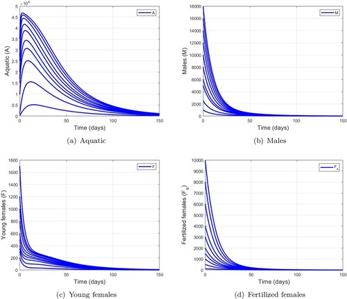
Figure 4 shows the trajectories of model (1(1) $\{\begin{array}{l}\dot{A}\left(t\right)=\mathrm{\rho \varphi }(1-{\displaystyle \frac{A\left(t\right)}{\mathrm{\theta K}}})F_s\left(t\right)-({\nu }_A+\omega +{\mu }_A)A\left(t\right),\\ \dot{M}\left(t\right)=(1-r)\lambda {\nu }_{A}A\left(t\right)-{\mu }_{M}M\left(t\right),\\ \dot{F}\left(t\right)=\mathrm{r\lambda }{\nu }_{A}A\left(t\right)-(\text{β}+{\mu }_F)F\left(t\right),\\ {\dot{F}}_s\left(t\right)=\text{β}{\displaystyle \frac{M\left(t\right)}{M\left(t\right)+F\left(t\right)}F\left(t\right)-{\mu }_{F_s}{F}_s\left(t\right),}\end{array}$(1) ) when $\mathcal{N}>1$. These trajectories converge towards the unique non-trivial equilibrium ${\mathcal{E}}_1$. Hence, mosquito populations persist in the environment. These numerical verifications illustrate the result stated in the Theorem 2.5.

5.1.2. Dynamics of wild mosquitoes with larvicide control only

The most common larviciding treatment is the use of temephos (Abate) and Bacillus thuringiensis israelensis [34, 48]. Here, we have assumed that larvicide spraying takes place at least once every 15 days over a period of 150 days. For this, we fixed $\theta =1$ and consider $\varphi =10,K=\mathrm{50,000},{\nu }_A=0.1,r=0.5,{\mu }_A=0.0583,{\mu }_M=1/10,\text{β}=0.7$, ${\mu }_F=1/7$, $\rho =1$, $\lambda =1$ and ${\mu }_{F_s}=1/10$. The simulations showing the effectiveness of the larvicide treatment are presented in Figure 5. We note that the population of mosquitoes in the aquatic stage is more affected than those in the aldute stage as shown in Table 5. We also observe that the effectiveness of larvicidal treatments has an impact on the basic offspring number, $\mathcal{N}$, more precisely it decreases when the larvicidal control parameter increases.

Figure 4. Simulation of model (1(1) $\{\begin{array}{l}\dot{A}\left(t\right)=\mathrm{\rho \varphi }(1-{\displaystyle \frac{A\left(t\right)}{\mathrm{\theta K}}})F_s\left(t\right)-({\nu }_A+\omega +{\mu }_A)A\left(t\right),\\ \dot{M}\left(t\right)=(1-r)\lambda {\nu }_{A}A\left(t\right)-{\mu }_{M}M\left(t\right),\\ \dot{F}\left(t\right)=\mathrm{r\lambda }{\nu }_{A}A\left(t\right)-(\text{β}+{\mu }_F)F\left(t\right),\\ {\dot{F}}_s\left(t\right)=\text{β}{\displaystyle \frac{M\left(t\right)}{M\left(t\right)+F\left(t\right)}F\left(t\right)-{\mu }_{F_s}{F}_s\left(t\right),}\end{array}$(1) ) using various initial condition when $\varphi =10,K=\mathrm{50,000},\theta =1,{\nu }_A=0.1,r=0.5,{\mu }_A=0.0583,\omega =0,{\mu }_M=1/10,\text{β}=0.7$, ${\mu }_F=1/7$, $\rho =1$, $\lambda =1$ and ${\mu }_{F_s}=1/10$ this leads to $\mathcal{N}=23.4499>1$. (a) Aquatic. (b) Males. (c) Young females and (d) Fertilized females.

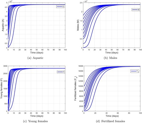
Figure 5. Dynamics of mosquito population using different values of larvicide control. (a) Aquatic. (b) Males. (c) Young females and (d) Ferlized females.

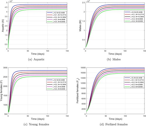
Table 5. Non-trivial equilibrium ${\mathcal{E}}_1=(A^{\ast },M^{\ast },F^{\ast },F_s^{\ast })$ of wild mosquitoes with different larvicide control values.

$\mathrm{\%}{m}_c$	ω	$\mathcal{N}$	$A^{\ast }$	$M^{\ast }$	$F^{\ast }$	$F_s^{\ast }$
$0\mathrm{\%}$	0	23.4499	$\mathrm{47,900}$	$\mathrm{23,930}$	2839	$\mathrm{17,770}$
$0\mathrm{\%}$	0.1	14.3714	$\mathrm{46,520}$	$\mathrm{23,260}$	2760	$\mathrm{17,270}$
$0\mathrm{\%}$	0.2	10.3664	$\mathrm{45,190}$	$\mathrm{22,590}$	2680	$\mathrm{16,770}$
$0\mathrm{\%}$	0.3	8.0998	$\mathrm{43,810}$	$\mathrm{21,910}$	2600	$\mathrm{16,270}$
$0\mathrm{\%}$	0.4	6.6490	$\mathrm{42,480}$	$\mathrm{21,240}$	2520	$\mathrm{15,770}$

5.1.3. Dynamics of wild mosquitoes with mechanical control only

Mechanical control $\left(m_c\right)$ is a type of intervention that involves destroying mosquito breeding sites to slow the growth of the immature form of the mosquito population. It has been shown that mechanical control $\left(m_c\right)$ can be an effective control tool [34, 57]. It is an inexpensive form of control, but requires the support of the local population. We assume that mechanical control $\left(m_c\right)$ leads to a decrease in K, i.e. a decrease in the equilibrium of the wild aquatic stage $A^{\ast }$. From relationship (8(8) $\{\begin{array}{l}{A}^{\ast }={\displaystyle \frac{{\mu }_M{M}^{\ast }}{(1-r)\lambda {\nu }_A},}\\ M^{\ast }={\displaystyle \frac{(1-r)(\mathcal{N}-1)\lambda {\nu }_A\mathrm{\theta K}}{{\mu }_M\mathcal{N}},}\\ F^{\ast }={\displaystyle \frac{r{\mu }_M{M}^{\ast }}{(1-r)(\text{β}+{\mu }_F)},}\\ F_s^{\ast }={\displaystyle \frac{r{\mu }_M\text{β}{M}^{\ast }}{{\mu }_{F_s}\left[\right(1-r\left)\right(\text{β}+{\mu }_F)+r{\mu }_M]}.}\end{array}$(8) ), we deduce that reducing $A^{\ast }$ for $m_c\mathrm{\%}$ corresponds to a decrease in K as follows $K=\frac{\mathcal{N}{A}^{\ast }}{(\mathcal{N}-1)(1-\frac{m_c}{100})},\mathrm{with}\theta =1-\frac{m_c}{100}.$We assume that the effectiveness of mechanical control does not depend on the seasons and should be applied as soon as possible. Thus, θ is defined as being between $(0,1]$, and the numerical simulation is carried out for 150 days. For this, we fixed $\omega =0$ and consider $\varphi =10,K=\mathrm{50,000},{\nu }_A=0.1,r=0.5,{\mu }_A=0.0583,{\mu }_M=1/10,\text{β}=0.7$, ${\mu }_F=1/7,{\mu }_{F_s}=1/10$, $\rho =1$, $\lambda =1$. We use the following initial conditions: $A\left(0\right)=1000,M\left(0\right)=1000,F\left(0\right)=1000,F_s\left(0\right)=1000$. The results of the numerical simulation for the effectiveness of mechanical control is shown in Figure 7. We observe that the mosquito population decreases when the level of mechanical control parameter increases. These figures show that this method of mechanical control is appropriate to fight against the proliferation of mosquitoes, especially in their immature stage as indicated in Table 6.

Table 6. Non-trivial equilibrium ${\mathcal{E}}_1=(A^{\ast },M^{\ast },F^{\ast },F_s^{\ast })$ of wild mosquitoes with different mechanic control values.

$\mathrm{\%}{m}_c$	ω	$\mathcal{N}$	$A^{\ast }$	$M^{\ast }$	$F^{\ast }$	$F_s^{\ast }$
$0\mathrm{\%}$	0	23.4499	$\mathrm{47,900}$	$\mathrm{23,930}$	2839	$\mathrm{17,770}$
$10\mathrm{\%}$	0	23.4499	$\mathrm{43,070}$	$\mathrm{21,540}$	2556	$\mathrm{15,990}$
$20\mathrm{\%}$	0	23.4499	$\mathrm{38,310}$	$\mathrm{19,150}$	2272	$\mathrm{14,220}$
$30\mathrm{\%}$	0	23.4499	$\mathrm{33,510}$	$\mathrm{16,750}$	1988	$\mathrm{12,440}$
$40\mathrm{\%}$	0	23.4499	$\mathrm{28,720}$	$\mathrm{14,360}$	1703	$\mathrm{10,660}$

5.1.4. Dynamics of wild mosquitoes with mechanical and larvicide control

We varied parameter $\theta ,\omega$ and fixed $\varphi =10,K=\mathrm{50,000},{\nu }_A=0.1,r=0.5,{\mu }_A=0.0583,{\mu }_M=1/10,\text{β}=0.7$, ${\mu }_F=1/7,{\mu }_{F_s}=1/10$, $\rho =1$, $\lambda =1$. Figure 6 shows the impact of the combination of mechanical and larvicide control. Moreover, these figures show interesting results that are better than mechanical control in Figure 7 and larviciding in Figure 5. We observe that when larval capacity is reduced by $50\mathrm{\%}$ ($\theta =0.5$) with low larviciding control ($\omega =0.05$), the mosquito population decreases to a significantly lower level than with high larviciding control ($\omega =0.25$) and low mechanical control $10\mathrm{\%}$ ($\theta =0.90$) as show in Table 7. Thus, this combined control could have a greater impact on reducing the growth dynamics of wild mosquitoes.

Figure 6. Dynamics of mosquito population using different values of mechanical and larvicide controls. (a) Aquatic. (b) Males. (c) Young females and (d) Ferlized females.

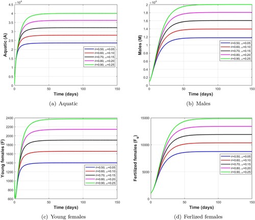
Figure 7. Dynamics of mosquito population using different values of mechanical control. (a) Aquatic. (b) Males. (c) Young females and (d) Ferlized females.

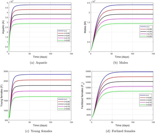
Table 7. Non-trivial equilibrium ${\mathcal{E}}_1=(A^{\ast },M^{\ast },F^{\ast },F_s^{\ast })$ of wild mosquitoes with different mechanic and larvicide control values.

$\mathrm{\%}{m}_c$	ω	$\mathcal{N}$	$A^{\ast }$	$M^{\ast }$	$F^{\ast }$	$F_s^{\ast }$
$50\mathrm{\%}$	0.05	17.8210	$\mathrm{23,580}$	$\mathrm{11,800}$	1400	8759
$40\mathrm{\%}$	0.10	14.3714	$\mathrm{27,920}$	$\mathrm{13,960}$	1656	$\mathrm{10,360}$
$30\mathrm{\%}$	0.15	12.0406	$\mathrm{32,100}$	$\mathrm{16,050}$	1904	$\mathrm{11,910}$
$20\mathrm{\%}$	0.20	10.3604	$\mathrm{36,120}$	$\mathrm{18,070}$	2144	$\mathrm{13,420}$
$10\mathrm{\%}$	0.25	9.0617	$\mathrm{40,030}$	$\mathrm{20,020}$	2376	$\mathrm{14,870}$

5.2. Numerical simulation of mosquito dynamics with constant releases of Wolbachia-infected male mosquitoes

In this section, we test different possible scenarios to reduce or eradicate the population of wild mosquitoes. Specifically, we have considered the following cases:

1. different release quantities of Wolbachia-infected male mosquitoes,

2. the influence of a combination of Wolbachia-infected male mosquitoes release, mechanical control and larvicide treatment on the growth dynamics of wild mosquitoes.

5.2.1. Dynamics of mosquito population with constant release without mechanical and larvicide control

We evaluate in this subsection the impact of different release rates of Wolbachia-infected male mosquitoes on wild mosquito populations. We use the following initial conditions: $A\left(0\right)=1000,M\left(0\right)=2000,F\left(0\right)=500,F_s\left(0\right)=1500,F_{\mathrm{st}}\left(0\right)=1$. The parameters used are: $\varphi =10,K=\mathrm{50,000},\theta =1,{\nu }_A=0.1,r=0.5,{\mu }_A=0.0583,\omega =0,{\mu }_M=1/10,\text{β}=0.7$, ${\mu }_F=1/7,{\mu }_{F_s}=1/10,{\mu }_i=0.12,{\mu }_{\mathrm{st}}=1/10$, $\rho =1$, $\lambda =1$ and the following release rates are assumed: $\mathrm{\Lambda }=\mathrm{10,000},\mathrm{12,500},\mathrm{15,000},\mathrm{17,500}$ which verifies the condition $M_i^{\ast }\in [0,M_i^{\mathrm{crit}})$ as indicated in Table 8. Thus, according to Theorem 3.3, system (11(11) $\{\begin{array}{l}\dot{A}\left(t\right)=\mathrm{\rho \varphi }(1-{\displaystyle \frac{A\left(t\right)}{\mathrm{\theta K}}})F_s\left(t\right)-({\nu }_A+\omega +{\mu }_A)A\left(t\right),\\ \dot{M}\left(t\right)=(1-r)\lambda {\nu }_{A}A\left(t\right)-{\mu }_{M}M\left(t\right),\\ \dot{F}\left(t\right)=\mathrm{r\lambda }{\nu }_{A}A\left(t\right)-(\text{β}+{\mu }_F)F\left(t\right),\\ {\dot{F}}_s\left(t\right)={\displaystyle \frac{\text{β}M\left(t\right)}{M\left(t\right)+M_i\left(t\right)+F\left(t\right)}F\left(t\right)-{\mu }_{F_s}{F}_s\left(t\right),}\\ {\dot{M}}_i\left(t\right)=\mathrm{\Lambda }-{\mu }_i{M}_i\left(t\right).\end{array}$(11) ) admits two positive equilibra points ${\mathcal{E}}_3^{-}$ given in Table 9 and ${\mathcal{E}}_3^{+}$ given in Table 8. By verifying the stability conditions given in Table 10, we conclude that equilibrium ${\mathcal{E}}_3^{-}$ is unstable and equilibrium ${\mathcal{E}}_3^{+}$ is locally stable, so the model solutions approach equilibrium ${\mathcal{E}}_3^{+}$ as shown in Figure 8 which confirms our analytical results stated in Theorem 3.4.

Figure 8. The effect of the release rate of Wolbachia-infected male mosquitoes without mechanical control and larvicide treatment on the population of wild mosquitoes with $M_i^{\ast }\in (0,M_i^{\mathrm{crit}})$ as indicated in Table 8. (a) Aquatic. (b) Males. (c) Young females. (d) Ferlized females and (e) Sterile females.

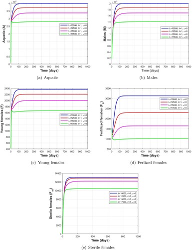
Table 8. Equilibrium point ${\mathcal{E}}_3^{+}$ for different values of Wolbachia-infected male releases $M_i^{\ast }\in (0,M_i^{\mathrm{crit}})$ with $\mathrm{\%}{m}_c=0$ and $\omega =0$.

Λ	$M_i^{\mathrm{crit}}$	$M_i^{\ast }$	$A^{\ast \ast }$	$M^{\ast \ast }$	$F^{\ast \ast }$	$F_s^{\ast \ast }$	$F_{\mathrm{st}}^{\ast \ast }$
$\mathrm{10,000}$	$1.5027\times {10}^5$	$8.3333\times {10}^4$	$\mathrm{39,910}$	$\mathrm{19,950}$	2367	3130	$\mathrm{13,070}$
$\mathrm{12,500}$	$1.5027\times {10}^5$	$1.0417\times {10}^5$	$\mathrm{37,190}$	$\mathrm{18,600}$	2206	2298	$\mathrm{12,870}$
$\mathrm{15,000}$	$1.5027\times {10}^5$	$1.25\times {10}^5$	$\mathrm{33,750}$	$\mathrm{16,870}$	2003	1644	$\mathrm{12,180}$
$\mathrm{17,500}$	$1.5027\times {10}^5$	$1.4583\times {10}^5$	$\mathrm{28,040}$	$\mathrm{14,020}$	1664	1011	$\mathrm{10,510}$

Table 9. Equilibrium point ${\mathcal{E}}_3^{-}$ for different values ofWolbachia-infected male releases $M_i^{\ast }\in (0,M_i^{\mathrm{crit}})$ with $\mathrm{\%}{m}_c=0$ and $\omega =0$.

Λ	$M_i^{\mathrm{crit}}$	$M_i^{\ast }$	$A^{\ast \ast }$	$M^{\ast \ast }$	$F^{\ast \ast }$	$F_s^{\ast \ast }$	$F_{\mathrm{st}}^{\ast \ast }$
$\mathrm{10,000}$	$1.5027\times {10}^5$	$8.3333\times {10}^4$	7960.3	3980.2	427.2235	149.8729	3137.9
$\mathrm{12,500}$	$1.5027\times {10}^5$	$1.0417\times {10}^5$	$\mathrm{10,677}$	5338.7	633.4036	214.918	4193.4
$\mathrm{15,000}$	$1.5027\times {10}^5$	$1.25\times {10}^5$	$\mathrm{14,120}$	7059.9	837.6163	311.4766	5514.9
$\mathrm{17,500}$	$1.5027\times {10}^5$	$1.4583\times {10}^5$	$\mathrm{19,823}$	9911.7	1176	519.9426	7650.1

Table 10. Numerical values verifying the condition of stability of the non-trivial equilibrium for the case of Figure 8.

$\mathcal{N}$	Λ	$M_i^{\ast }$	$M_1^{\ast \ast }$	$g\left(M_1^{\ast \ast }\right)$	$M_{-}^{\ast \ast }$	$M_{+}^{\ast \ast }$
23.4499	$\mathrm{10,000}$	$8.3333\times {10}^4$	8911.7	$-\mathrm{51,078}$	3680.2	$\mathrm{19,950}$
23.4499	$\mathrm{12,500}$	$1.0417\times {10}^5$	9963.6	$-\mathrm{37,445}$	5338.7	$\mathrm{18,600}$
23.4499	$\mathrm{15,000}$	$1.25\times {10}^5$	$\mathrm{10,915}$	$-\mathrm{21,547}$	7059.9	$\mathrm{16,870}$
23.4499	$\mathrm{17,500}$	$1.4583\times {10}^5$	$\mathrm{11,789}$	$-3932.7$	9911.7	$\mathrm{14,020}$

Figure 8 shows the total number of mosquitoes in the aquatic stage, wild males, young females, fertile females and the number of Wolbachia-infected female mosquitoes. When the release rate is increased from $\mathrm{10,000}$ to $\mathrm{17,500}$, we observe that the total number of mosquitoes in the aquatic stage, wild male, young female and fertile female stages decreases to a significantly lower level. Thus, when a large number of Wolbachia-infected male mosquitoes are released, this will result in a significant reduction in the wild mosquito population.

5.2.2. Dynamics of mosquito population with constant release, mechanical and larvicide control

In this subsection, we evaluate the constant release of Wolbachia-infected males in combination with mechanical control and larvicide treatment.

Figure 9 shows the effect of the release rate of Wolbachia-infected male mosquitoes combined mechanical control with larvicide treatment on the population of wild mosquitoes with $M_i^{\ast }\in (0,M_i^{\mathrm{crit}})$ as indicated in Table 11. By comparing the numerical results in Tables 8 and 11, we find that a release of Wolbachia-infected males mosquitoes $\mathrm{10,000}$ with a mechanical control of $20\mathrm{\%}$ and a larvicide treatment of 0.05 gives better results than a release of $\mathrm{17,500}$ Wolbachia-infected males mosquitoes without control measures.

5.3. Numerical simulation of mosquito dynamics with impulsive releases of Wolbachia-infected male mosquitoes

In this section, we simulate different possible scenarios to reduce or eradicate the population of wild mosquitoes by the impulsive release of Wolbachia-infected males. More specifically, we considered the following cases:

1. different release periodicities,

2. different quantities of Wolbachia-infected male mosquitoes for each fixed period,

3. the influence of a combination of impulsive release of Wolbachia-infected male mosquitoes, mechanical control and larvicide treatment on the growth dynamics of wild mosquitoes.

Figure 9. The effect of the release rate of Wolbachia-infected male mosquitoes combined mechanical control and larvicide treatment on the population of wild mosquitoes with $M_i^{\ast }\in (0,M_i^{\mathrm{crit}})$ as indicated in Table 11. (a) Aquatic. (b) Males. (c) Young females. (d) Ferlized females and (e) Sterile females.

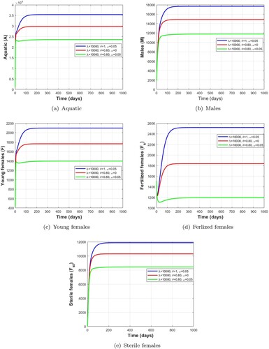
Figure 10. Dynamics of impulsive release of Wolbachia-infected male on the mosquito population when $T=14,\mathrm{\Lambda }=\mathrm{50,000},\mathrm{150,000}$ which verifies the conditions given in Table 12. (a) Aquatic. (b) Males. (c) Young females. (d) Ferlized females. (e) Sterile females and (f) Sterile males.

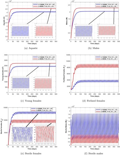
Table 11. Impact of the constant release of Wolbachia-infected males combined with mechanical control and larvicidal treatment on mosquito dynamics with $\mathrm{\Lambda }=\mathrm{10,000}$.

$\mathrm{\%}{m}_c$	ω	$\mathcal{N}$	$M_i^{\mathrm{crit}}$	$M_i^{\ast }$	$A^{\ast \ast }$	$M^{\ast \ast }$	$F^{\ast \ast }$	$F_s^{\ast \ast }$	$F_{\mathrm{st}}^{\ast \ast }$
$0\mathrm{\%}$	0.05	17.8210	$1.1101\times {10}^5$	$\mathrm{83,333}$	$\mathrm{35,380}$	$\mathrm{17,690}$	2098	2520	$\mathrm{11,870}$
$20\mathrm{\%}$	0	23.4499	$1.2021\times {10}^5$	$\mathrm{83,333}$	$\mathrm{29,750}$	$\mathrm{14,880}$	1765	1838	$\mathrm{10,300}$
$20\mathrm{\%}$	0.05	17.8210	$8.8804\times {10}^4$	$\mathrm{83,333}$	$\mathrm{23,570}$	$\mathrm{11,780}$	1398	1194	8448

Table 12. Numerical values verifying the condition of existence and stability of the non-trivial periodic solution, (i.e. $\mathcal{N}>1$, $T>T^{\ast }$ and $\mathrm{\Lambda }<{\mathrm{\Lambda }}^{\ast }$) for the case of Figure 10.

T	$T^{\ast }$	Λ	${\mathrm{\Lambda }}^{\ast }$	$\mathrm{\%}{m}_c$	ω	$\mathcal{N}$
14	5.7689	$\mathrm{150,000}$	655, 990	$0\mathrm{\%}$	0	23.4499
14	2.3937	$\mathrm{50,000}$	655, 990	$0\mathrm{\%}$	0	23.4499

5.3.1. Dynamics of mosquito population with impulsive releases without mechanical and larvicide control

In this subsection to illustrate our theoretical results, we use the following values $\theta =1,\omega =0,\varphi =10,K=\mathrm{50,000},{\nu }_A=0.1,r=0.5,{\mu }_A=0.0583,{\mu }_M=1/10,\text{β}=0.7$, ${\mu }_F=1/7,{\mu }_{F_s}=1/10,{\mu }_i=0.12,{\mu }_{\mathrm{st}}=1/10$, $\rho =1$, $\lambda =1$.

In the case of Figure 10, we choose a pulse period T = 14 days and the number of Wolbachia-infected male mosquitoes release $\mathrm{\Lambda }=\mathrm{50,000}$ and $\mathrm{150,000}$. Moreover, in the case of Figure 11, we take a pulse period T = 21 days and the number of Wolbachia-infected male mosquitoes release $\mathrm{\Lambda }=\mathrm{50,000}$ and $\mathrm{150,000}$. Thus, using these parameters, we have $\mathcal{N}>1$, $T>T^{\ast }$ and $\mathrm{\Lambda }<{\mathrm{\Lambda }}^{\ast }$, as indicated by the numerical values obtained in Tables 12 and 15. Then, according to Theorem 4.7, system (20(20) $\{\begin{array}{l}\begin{array}{l}\dot{A}\left(t\right)=\mathrm{\rho \varphi }(1-{\displaystyle \frac{A\left(t\right)}{\mathrm{\theta K}}})F_s\left(t\right)-({\nu }_A+\omega +{\mu }_A)A\left(t\right)\\ \dot{M}\left(t\right)=(1-r)\lambda {\nu }_{A}A\left(t\right)-{\mu }_{M}M\left(t\right)\\ \dot{F}\left(t\right)=\mathrm{r\lambda }{\nu }_{A}A\left(t\right)-(\text{β}+{\mu }_F)F\left(t\right)\\ {\dot{F}}_s\left(t\right)={\displaystyle \frac{\text{β}M\left(t\right)}{M\left(t\right)+M_i\left(t\right)+F\left(t\right)}F\left(t\right)-{\mu }_{F_s}{F}_s\left(t\right)}\\ {\dot{M}}_i\left(t\right)=-{\mu }_i{M}_i\left(t\right),\end{array}\}t\ne \mathrm{nT}\\ \begin{array}{l}A\left(n{T}^{+}\right)=A\left(\mathrm{nT}\right),\\ M\left(n{T}^{+}\right)=M\left(\mathrm{nT}\right),\\ F\left(n{T}^{+}\right)=F\left(\mathrm{nT}\right),\\ F_s\left(n{T}^{+}\right)=F_s\left(\mathrm{nT}\right),\\ M_i\left(n{T}^{+}\right)=M_i\left(\mathrm{nT}\right)+\mathrm{\Lambda },\end{array}\}t=\mathrm{nT}\mathrm{with}n=1,2,\dots ,N_T.\end{array}$(20) ) has two positive non-trivial periodic solutions ${\mathcal{E}}_{-}^{\ast }\left(t\right)=\left(A_{-}^{\ast }\right(t),M_{-}^{\ast }(t),F_{-}^{\ast }(t),F_{s-}^{\ast }(t),M_i^{\mathrm{per}}(t\left)\right)$ and ${\mathcal{E}}_{+}^{\ast }\left(t\right)=\left(A_{+}^{\ast }\right(t),M_{+}^{\ast }(t),F_{+}^{\ast }(t),F_{s+}^{\ast }(t),M_i^{\mathrm{per}}(t\left)\right)$ . Moreover, ${\mathcal{E}}_{-}^{\ast }\left(t\right)=\left(A_{-}^{\ast }\right(t),M_{-}^{\ast }(t),F_{-}^{\ast }(t),F_{s-}^{\ast }(t),M_i^{\mathrm{per}}(t\left)\right)$ is an unstable non-trivial periodic solution and ${\mathcal{E}}_{+}^{\ast }\left(t\right)=\left(A_{+}^{\ast }\right(t),M_{+}^{\ast }(t),F_{+}^{\ast }(t),F_{s+}^{\ast }(t),M_i^{\mathrm{per}}(t\left)\right)$ is a locally asymptotically stable non-trivial periodic solution. Additionally, the range of existence of a stable non-trivial periodic solution is given in Tables 13, 14, 16 and 17. We observe in the Figures 10 and 11 that the number of mosquitoes in the aquatic stage, wild males, young females and fertile females decreases as release pulses increase, while Wolbachia-infected female mosquitoes increase, leading to a reduction in the wild mosquito population.

Remark 5.1

From the numerical results obtained in Tables 13, 14, 16, 17 and Figures 10, 11 we can deduce that a short pulse period and a higher number of releases of Wolbachia-infected male mosquitoes are the best way to quickly reduce wild mosquito population.

Figure 11. Dynamics of impulsive release of Wolbachia-infected male on the mosquito population when $T=21,\mathrm{\Lambda }=\mathrm{50,000},\mathrm{150,000}$ which verifies the conditions given in Table 15. (a) Aquatic. (b) Males. (c) Young females. (d) Ferlized females. (e) Sterile females and (f) Sterile males.

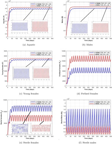
Table 13. The range of existence of a stable non-trivial periodic solution when T = 14 and $\mathrm{\Lambda }=\mathrm{150,000}$ for Figure 10 (blue colour).

A	M	F	$F_s$	$F_{\mathrm{st}}$	$M_i$
$[\mathrm{40,360},\mathrm{41,560}]$	$[\mathrm{20,360},\mathrm{20,480}]$	$[2397,2457]$	$[3296,4039]$	$[\mathrm{12,410},\mathrm{13,310}]$	$[\mathrm{34,360},\mathrm{184,400}]$

Table 14. The range of existence of a stable non-trivial periodic solution when T = 14 and $\mathrm{\Lambda }=\mathrm{50,000}$ for Figure 10 (red colour).

A	M	F	$F_s$	$F_{\mathrm{st}}$	$M_i$
$[\mathrm{45,460},\mathrm{45,990}]$	$[\mathrm{22,800},\mathrm{22,850}]$	$[2698,2724]$	$[7921,9092]$	$[\mathrm{28,060},\mathrm{29,420}]$	$[\mathrm{11,450},\mathrm{61,450}]$

Table 15. Numerical values verifying the condition of existence and stability of the non-trivial periodic solution (i.e. $\mathcal{N}>1$, $T>T^{\ast }$ and $\mathrm{\Lambda }<{\mathrm{\Lambda }}^{\ast }$) for the case of Figure 11.

T	$T^{\ast }$	Λ	${\mathrm{\Lambda }}^{\ast }$	$\mathrm{\%}{m}_c$	ω	$\mathcal{N}$
21	5.7689	$\mathrm{150,000}$	$1.7173\times {10}^6$	$0\mathrm{\%}$	0	23.4499
21	2.3937	$\mathrm{50,000}$	$1.7173\times {10}^6$	$0\mathrm{\%}$	0	23.4499

Table 16. The range of existence of a stable non-trivial periodic solution when T = 21 and $\mathrm{\Lambda }=\mathrm{150,000}$ for Figure 11 (blue colour).

A	M	F	$F_s$	$F_{\mathrm{st}}$	$M_i$
$[\mathrm{43,410},\mathrm{45,070}]$	$[\mathrm{21,920},\mathrm{22,160}]$	$[2576,2667]$	$[5193,7417]$	$[\mathrm{33,210},\mathrm{35,870}]$	$[\mathrm{13,120},\mathrm{163,100}]$

Table 17. The range of existence of a stable non-trivial periodic solution when T = 21 and $\mathrm{\Lambda }=\mathrm{50,000}$ for Figure 11 (red colour).

A	M	F	$F_s$	$F_{\mathrm{st}}$	$M_i$
$[\mathrm{46,230},\mathrm{46,910}]$	$[\mathrm{23,210},\mathrm{23,310}]$	$[2744,2780]$	$[9758,\mathrm{12,140}]$	$[\mathrm{20,520},\mathrm{23,350}]$	$[4375,\mathrm{54,370}]$

5.3.2. Dynamics of mosquito population with impulsive releases, mechanical and larvicide control

Now, we evaluate impulsive release of Wolbachia-infected males combined with mechanical control and larvicide treatment.

In Figure 12 (resp. Figure 13), we choose an impulse period T = 14 days (resp. T = 21 days), $\mathrm{\Lambda }=\mathrm{50,000}$, $\theta =0.70$ and $\omega =0.1$ (curves in red), then we consider $\mathrm{\Lambda }=\mathrm{150,000}$, $\theta =1$ and $\omega =0$ (curves in blue). Thus, using the parameters given in Table 3, we have $\mathcal{N}>1$, $T>T^{\ast }$ and $\mathrm{\Lambda }<{\mathrm{\Lambda }}^{\ast }$, as indicated by the numerical values obtained in Table 18 (resp. Table 19). Moreover, using the same interpretation argument from Section 5.3.1 we can deduce that the non-trivial periodic solution ${\mathcal{E}}_{+}^{\ast }\left(t\right)=\left(A_{+}^{\ast }\right(t),M_{+}^{\ast }(t),F_{+}^{\ast }(t),F_{s+}^{\ast }(t),M_i^{\mathrm{per}}(t\left)\right)$ is locally asymptotically stable. In Figures 12 and 13, we observe that the release of $\mathrm{50,000}$ Wolbachia-infected males combined with a mechanical control of $30\mathrm{\%}(\theta =0.70)$ and a larvicidal treatment that eliminates the population of aquatic stage mosquitoes by $10\mathrm{\%}(\omega =0.1)$ is significantly better than the release of $\mathrm{150,000}$ Wolbachia-infected males without a mechanical control and larvicide treatment.

Remark 5.2

The numerical results obtained in Tables 13, 14, 16, 17, 18, 19 and Figures 10, 11, 12, 13 allow us to deduce that a long pulse period with a lower number of releases of Wolbachia-infected male mosquitoes combined with mechanical control and larviciding is a better way of rapidly reducing the wild mosquito population than a huge number of male releases over a short period.

Figure 12. Dynamics of the impulsive release of a Wolbachia-infected male on the mosquito population with mechanical and larvicide control when $T=14,\mathrm{\Lambda }=\mathrm{50,000},\mathrm{150,000}$ verifying the conditions given in Table 18. (a) Aquatic. (b) Males. (c) Young females. (d) Ferlized females. (e) Sterile females and (f) Sterile males.

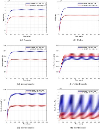
Figure 13. Dynamics of the impulsive release of a Wolbachia-infected male on the mosquito population with mechanical and larvicide control when $T=21,\mathrm{\Lambda }=\mathrm{50,000},\mathrm{150,000}$ verifying the conditions given in Table 19. (a) Aquatic. (b) Males. (c) Young females. (d) Ferlized females. (e) Sterile females and (f) Sterile males.

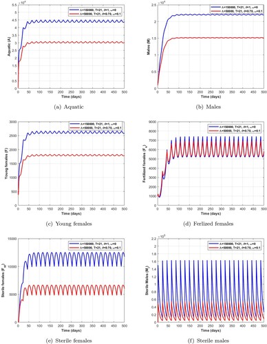
Table 18. Numerical values verifying the condition of existence and stability of the non-trivial periodic solution, (i.e. $\mathcal{N}>1$, $T>T^{\ast }$ and $\mathrm{\Lambda }<{\mathrm{\Lambda }}^{\ast }$) for the case of Figure 12.

T	$T^{\ast }$	Λ	${\mathrm{\Lambda }}^{\ast }$	$\mathrm{\%}{m}_c$	ω	$\mathcal{N}$
14	5.7689	$\mathrm{150,000}$	$6.5599\times {10}^5$	$0\mathrm{\%}$	0	23.4499
14	4.9958	$\mathrm{50,000}$	$2.6580\times {10}^5$	$30\mathrm{\%}$	0.1	14.3714

Table 19. Numerical values verifying the condition of existence and stability of the non-trivial periodic solution, (i.e. $\mathcal{N}>1$, $T>T^{\ast }$ and $\mathrm{\Lambda }<{\mathrm{\Lambda }}^{\ast }$) for the case of Figure 13.

T	$T^{\ast }$	Λ	${\mathrm{\Lambda }}^{\ast }$	$\mathrm{\%}{m}_c$	ω	$\mathcal{N}$
21	5.7689	$\mathrm{150,000}$	$1.7173\times {10}^6$	$0\mathrm{\%}$	0	23.4499
21	4.9958	$\mathrm{50,000}$	$6.9585\times {10}^5$	$30\mathrm{\%}$	0.1	14.3714

6. Conclusion

Due to the absence of effective clinical treatments and vaccines, current methods of controlling vector-borne diseases are mainly aimed at eradicating the main mosquito vectors. However, traditional means, including larval source reduction and insecticide application, are not sufficient to keep vector population densities below the epidemic risk threshold. In recent years, a very promising strategy has been to release Wolbachia-infected male mosquitoes into wild areas in order to sterilize wild female mosquitoes through cytoplasmic incompatibility.

In this work, we first presented a mathematical model (1(1) $\{\begin{array}{l}\dot{A}\left(t\right)=\mathrm{\rho \varphi }(1-{\displaystyle \frac{A\left(t\right)}{\mathrm{\theta K}}})F_s\left(t\right)-({\nu }_A+\omega +{\mu }_A)A\left(t\right),\\ \dot{M}\left(t\right)=(1-r)\lambda {\nu }_{A}A\left(t\right)-{\mu }_{M}M\left(t\right),\\ \dot{F}\left(t\right)=\mathrm{r\lambda }{\nu }_{A}A\left(t\right)-(\text{β}+{\mu }_F)F\left(t\right),\\ {\dot{F}}_s\left(t\right)=\text{β}{\displaystyle \frac{M\left(t\right)}{M\left(t\right)+F\left(t\right)}F\left(t\right)-{\mu }_{F_s}{F}_s\left(t\right),}\end{array}$(1) ) describing the dynamics of the wild mosquito population on the basis of its life cycle. Measures in terms of mechanical control and larviciding were considered to reduce the growth of wild mosquitoes. We have shown that the problem is well posed mathematically and biologically. We defined the basic offspring number $\mathcal{N}$. Specifically, we have shown that, depending on the basic offspring number $\mathcal{N}$, there is an equilibrium point corresponding to the extinction of the wild mosquito population and another corresponding to the persistence of the mosquito population in the environment. We have also shown that when $\mathcal{N}\ge 1$, the trivial equilibrium is globally asymptotically stable and when $\mathcal{N}>1$, there exists a unique non-trivial equilibrium that is globally asymptotically stable. Numerical simulations have been presented to illustrate and support the analytical results. Our numerical result suggests that mechanical control combined with mechanical treatment reduces significantly the wild mosquito population.

Next, we added a compartment of Wolbachia-infected male mosquitoes to this initial model (1(1) $\{\begin{array}{l}\dot{A}\left(t\right)=\mathrm{\rho \varphi }(1-{\displaystyle \frac{A\left(t\right)}{\mathrm{\theta K}}})F_s\left(t\right)-({\nu }_A+\omega +{\mu }_A)A\left(t\right),\\ \dot{M}\left(t\right)=(1-r)\lambda {\nu }_{A}A\left(t\right)-{\mu }_{M}M\left(t\right),\\ \dot{F}\left(t\right)=\mathrm{r\lambda }{\nu }_{A}A\left(t\right)-(\text{β}+{\mu }_F)F\left(t\right),\\ {\dot{F}}_s\left(t\right)=\text{β}{\displaystyle \frac{M\left(t\right)}{M\left(t\right)+F\left(t\right)}F\left(t\right)-{\mu }_{F_s}{F}_s\left(t\right),}\end{array}$(1) ). In order to evaluate the effects of constant releases of Wolbachia-infected male mosquitoes on the wild mosquito population. In addition, we considered mechanical control and larviciding to assess its impact on mosquito dynamics. We obtained a critical threshold number of releases of Wolbachia-infected male mosquitoes, $M_i^{\mathrm{crit}}$ . Then, we established theoretically and numerically that the elimination of wild mosquitoes is possible when the number of Wolbachia-infected male mosquitoes released $M_i^{\ast }$ is greater than this threshold. In addition, below this threshold, we have determined properties of a global nature for system equilibria. We prove that when $M_i^{\ast }\in [0,M_i^{\mathrm{crit}})$ , the model admits exactly two equilibrium points; one of which is asymptotically stable and the other unstable. The trivial equilibrium, corresponding to the elimination of wild mosquitoes, is locally asymptotically stable, and becomes globally asymptotically stable when $\mathcal{N}\le 1$. Our numerical result suggests that releasingWolbachia-infected males in combination with mechanical control and larviciding is more efficient, as shown in Figure 9, since it reduces the number of Wolbachia-infected male mosquitoes initial to be released, which is economically beneficial.

Finally, we have established an impulse model of the interaction between Wolbachia-infected male mosquitoes and wild mosquito population. Firstly, it is found that there is always a trivial periodic solution corresponding to the extinction of mosquito populations, and the corresponding local and global stability conditions are given using Floquet theory and Lyapunov's stability theorem, respectively. Moreover, the results show that the impulsive release of Wolbachia-infected male mosquitoes can lead to the extinction of wild mosquitoes when $\mathcal{N}>1$, $T<T^{\ast }$ and $\mathrm{\Lambda }>{\mathrm{\Lambda }}^{\ast }$. Secondly, we find that there can be two solutions in the system when certain threshold conditions are met. The existence of non-trivial periodic solutions is then obtained, and its local stability is discussed when $\mathcal{N}>1$, $T>T^{\ast }$ and $\mathrm{\Lambda }<{\mathrm{\Lambda }}^{\ast }$. The analysis shows that there is only one non-trivial periodic solution which is locally asymptotically stable. The numerical results of the impulsive model show that a long pulse period with a lower number of releases of Wolbachia-infected male mosquitoes combined with mechanical control and larviciding Figures 12 and 13 is a better way of rapidly reducing the wild mosquito population than a huge number of male releases over a short period Figures 10 and 11.

Our results suggest that the release ofWolbachia-infected male mosquitoes, combined with mechanical control and larviciding, is one of the best ways of significantly reducing the wild mosquito population to a very low level. Indeed, control measures combined with releases reduce the cost of producing Wolbachia-infected male mosquitoes in the laboratory.

In our future work, we intend to use the optimal control approach to minimize the costs associated with controlling the mosquito population through the application of larvicides, by introducing the release of Wolbachia-infected male mosquitoes into the environment. In addition, we aim to couple these models to the transmission of malaria and other vector-borne diseases, in order to assess their impact on transmission.

Disclosure statement

No potential conflict of interest was reported by the author(s).

References

- Caraballo H, King K. Emergency department management of mosquito-borne illness: malaria, dengue, and West Nile virus. Emerg Med Pract. 2014;16(5):1–23.
- Tolle M. Mosquito-borne diseases. Curr Probl Pediatr Adolesc Health Care. 2009;39:97–140.
- Hemingway J, Ranson H. Insecticide resistance in insect vectors of human disease. Annu Rev Entomol. 2000;45:371–91. doi: 10.1146/ento.2000.45.issue-1
- Saha S, Dutta P, Samanta G. Dynamical behavior of SIRS model incorporating government action and public response in presence of deterministic and fluctuating environments. Chaos Solit Fractals. 2022;164:Article ID 112643. doi: 10.1016/j.chaos.2022.112643
- Traoré B, Sangaré B, Traoré S. A mathematical model of malaria transmission in a periodic environment. J Biol Dyn. 2018;12:400–432. doi: 10.1080/17513758.2018.1468935
- Engelstädter J, Telschow A. Cytoplasmic incompatibility and host population structure. J Hered. 2009;103:196–207. doi: 10.1038/hdy.2009.53
- Zheng B, Liu X, Tang M, et al. Use of age-stage structural models to seek optimal Wolbachia-infected male mosquito releases for mosquito-borne disease control. J Theor Biol. 2019;472:95–109. doi: 10.1016/j.jtbi.2019.04.010
- Bian G, Joshi D, Dong Y, et al. Wolbachia invades Anopheles stephensi populations and induces refractoriness to plasmodium infection. Science. 2013;340:748–751. doi: 10.1126/science.1236192
- Xianghong Z, Sanyi T, Robert AC. Models to assess how best to replace dengue virus vectors with Wolbachia-infected mosquito populations. Math Biosci. 2015;269:164–177. doi: 10.1016/j.mbs.2015.09.004
- Dutta P, Samanta G, Nieto JJ. Periodic transmission and vaccination effects in epidemic dynamics: a study using the SIVIS model. Nonlinear Dyn. 2024;112:2381–2409. doi: 10.1007/s11071-023-09157-4
- Koutou O, Traoré B, Sangaré B. Mathematical modeling of malaria transmission global dynamics: taking into account the immature stages of the vectors. Adv Differ Equ. 2018;2018(220):1–34.
- Saha S, Samanta G. Analysis of a host–vector dynamics of a dengue disease model with optimal vector control strategy. Math Comput Simul. 2022;195:31–55. doi: 10.1016/j.matcom.2021.12.021
- Sangaré B. Contribution à la modélisation mathématique en épidémiologie et en écologie et à la résolution numérique des EDP évolutives. Habilitation à Diriger des Recherches, Université Franche-Comté; 02 Juin 2023.
- Traoré B, Koutou O, Sangaré B. A global mathematical model of malaria transmission dynamics with structured mosquito population and temperature variations. Nonlinear Anal Real World Appl. 2020;53:Article ID 103081.
- Luz PM, Codeço CT, Medlock J, et al. Impact of insecticide interventions on the abundance and resistance profile of Aedes aegypti. Epidemiol Infect. 2009;137:1203–1215. doi: 10.1017/S0950268808001799
- Oki M, Sunahara T, Hashizume M, et al. Optimal timing of insecticide fogging to minimize dengue cases: modeling dengue transmission among various seasonalities and transmission intensities. PLoS Negl Trop Dis. 2011;5:1–7. doi: 10.1371/journal.pntd.0,001,367
- Alphey N, Alphey L, Bonsall MB. A model framework to estimate impact and cost of genetics-based sterile insect methods for dengue vector control. PLoS One. 2011;6:1–12. doi: 10.1371/journal.pone.0025384
- Anguelov R, Dumont Y, Lubuma J. Mathematical modeling of sterile insect technology for control of anopheles mosquito. Comput Math Appl. 2012;64:374–389. doi: 10.1016/j.camwa.2012.02.068
- Dumont Y, Yatat–Djeumen I. Sterile insect technique with accidental releases of sterile females. impact on mosquito-borne diseases control when viruses are circulating. Math Biosci. 2022;343:Article ID 108724. doi: 10.1016/j.mbs.2021.108724
- Huang M, Song X, Li J. Modelling and analysis of impulsive releases of sterile mosquitoes. J Biol Dyn. 2017;11:147–171. doi: 10.1080/17513758.2016.1254286
- Roberto CT, Mo YH, Lourdes E. Optimal control of Aedes aegypti mosquitoes by the sterile insect technique and insecticide. Math Biosci. 2010;223(1):12–23. doi: 10.1016/j.mbs.2009.08.009
- Strugarek M, Bossin H, Dumont Y. On the use of the sterile insect release technique to reduce or eliminate mosquito populations. Appl Math Model. 2018;68:443–470. doi: 10.1016/j.apm.2018.11.026
- Bliman P-A, Aronna M, Coelho F, et al. Ensuring successful introduction of Wolbachia in natural populations of Aedes aegypti by means of feedback control. J Math Biol. 2018;76:1269–1300. doi: 10.1007/s00285-017-1174-x
- Himanshu J, Arvind KS. Modeling the effect of Wolbachia to control malaria transmission. Expert Syst Appl. 2023;221:Article ID 119769.
- Hoffmann A, Montgomery B, Popovici J, et al. Successful establishment of Wolbachia in Aedes populations to suppress dengue transmission. Nature. 2011;476:454–457. doi: 10.1038/nature10356
- Jair K, Moacyr AHS, Max OS, et al. Aedes, Wolbachia and dengue; 2014.
- Putri Y, Rozi S, Tasman H, et al. Assessing the effect of extrinsic incubation period (EIP) prolongation in controlling dengue transmission with Wolbachia-infected mosquito intervention.AIP Conference Proceedings, Vol. 1825. Makassar, Indonesia. 2017.
- Arias J, Martínez H, Sepúlveda-Salcedo L, et al. Predator–prey model for analysis of Aedes aegypti population dynamics in Cali, Colombia. Int J Pure Appl Math. 2015;105(4):561–597. doi: 10.12732/ijpam.v105i4.2
- Zhongcai Z, Yuanxian H, Linchao H. The impact of predators of mosquito larvae on Wolbachia spreading dynamics. J Biol Dyn. 2023;17(1):Article ID 2249024.
- Nundloll S, Mailleret L, Grognard F. Two models of interfering predators in impulsive biological control. J Biol Dyn. 2010;4:102–114. doi: 10.1080/17513750902968779
- Pliego-Pliego E, Vasilieva O, Velázquez-Castro J, et al. Control strategies for a population dynamics model of Aedes aegypti with seasonal variability and their effects on dengue incidence. Appl Math Model. 2020;81:296–319. doi: 10.1016/j.apm.2019.12.025
- Dumont Y, Chiroleu F, Domerg C. On a temporal model for the Chikungunya disease: modeling, theory and numerics. Math Biosci. 2008;213(1):80–91. doi: 10.1016/j.mbs.2008.02.008
- Dumont Y, Tchuenche J. Mathematical studies on the sterile insect technique for the Chikungunya disease and Aedes albopictus. J Math Biol. 2012;65:809–854. doi: 10.1007/s00285-011-0477-6
- Hamdan N, Kilicman A. Mathematical modelling of dengue transmission with intervention strategies using fractional derivatives. Bull Math Biol. 2022;84:138. doi: 10.1007/s11538-022-01096-2
- Pulecio-Montoya A, López-Montenegro L, Medina-García J. Description and analysis of a mathematical model of population growth of Aedes aegypti. J Appl Math Comput. 2021;65:335–349. doi: 10.1007/s12190-020-01394-9
- Djeumen V, Couteron P, Jules TJ, et al. An impulsive modelling framework of fire occurrence in a size structured model of tree-grass interactions for savanna ecosystems. J Math Biol. 2017;74:1425–1482. doi: 10.1007/s00285-016-1060-y
- Miranda GAN, Teboh-Ewungkem I. Infectious diseases and our planet. Cham: Springer; 2021.
- Ngwa GA, Teboh-Ewungkem MI, Dumont Y, et al. On a three-stage structured model for the dynamics of malaria transmission with human treatment, adult vector demographics and one aquatic stage. J Theor Biol. 2019;481:202–222. doi: 10.1016/j.jtbi.2018.12.043
- Assefa WW, Rachid O, Jacek B. Mathematical analysis of the impact of transmission-blocking drugs on the population dynamics of malaria. Appl Math Comput. 2021;400:Article ID 126005.
- Howell P, Knols B. Male mating biology. Malar J. 2009;8(Suppl 2):S8. doi: 10.1186/1475-2875-8-S2-S8
- Diabaté A, Sangaré B, Koutou O. Mathematical modeling of the dynamics of vector-borne diseases transmitted by mosquitoes: taking into account aquatic stages and gonotrophic cycle. Nonauton Dyn Syst. 2022;9:205–236. doi: 10.1515/msds-2022-0155
- Diabaté A, Sangaré B, Koutou O. Optimal control analysis of a COVID-19 and tuberculosis (TB) co-infection model with an imperfect vaccine for covid-19. SeMA J. 2023;1–28. doi:10.1007/s40324-023-00330-8.
- Savadogo A, Sangaré B, Ouédraogo H. A mathematical analysis of Hopf-bifurcation in a prey–predator model with nonlinear functional response. Adv Differ Equ. 2021;2021:275. doi: 10.1186/s13662-021-03437-2
- Smith HL. Monotone dynamical systems: an introduction to the theory of competitive and cooperative systems. bull new series. Am Math Soc. 1996;33:203–209. doi: 10.1090/S0273-0979-96-00642-8
- Zhang X, Liu X, Li Y, et al. Modelling the effects of Wolbachia-carrying male augmentation and mating competition on the control of dengue fever. J Dyn Differ Equ. 2023;81:1–41.
- Koutou O, Diabaté A, Sangaré B. Mathematical analysis of the impact of the media coverage in mitigating the outbreak of covid-19. Math Comput Simul. 2022;205:600–618. doi: 10.1016/j.matcom.2022.10.017
- Savadogo A, Sangaré B, Ouédraogo H. A mathematical analysis of prey–predator population dynamics in the presence of an SIS infectious disease. RMS Res Math Stat. 2022;9:1–22.
- Iboi E, Gumel A, Taylor J. Mathematical modeling of the impact of periodic release of sterile male mosquitoes and seasonality on the population abundance of malaria mosquitoes. J Biol Syst. 2020;28:1–34. doi: 10.1142/S0218339020400033
- Ivanka S, Gani S. Applied impulsive mathematical models. Cham: Springer; 2016.
- Pang Y, Wang S. Dynamic analysis of the Wolbachia-infected male mosquitoes model by pulsed release. Adv Appl Math. 2021;10:3505–3517. doi: 10.12677/AAM.2021.1010370
- Pang Y, Wang S, Liu S. Dynamics analysis of stage-structured wild and sterile mosquito interaction impulsive model. J Biol Dyn. 2022;16:464–479. doi: 10.1080/17513758.2022.2079739
- Drumi DB, Pavel SS. Impulsive differential equations: periodic solutions and applications; 1993.
- Bainov D, Simeonov PS, Lakshmikantham V. Theory of impulsive differential equations. Plovdiv: Word Scientific Publishing; 1989.
- Korobeinikov A, Wake G. Lyapunov functions and global stability for SIR, SIRS, and SIS epidemiological models. Appl Math Lett. 2002;15(8):955–960. doi: 10.1016/S0893-9659(02)00069-1
- Manyombe MLM, Mbang J, Tsanou B, et al. Mathematical analysis of a spatiotemporal model for the population ecology of anopheles mosquito. Math Methods Appl Sci. 2020;43:3524–3555. doi: 10.1002/mma.v43.6
- Hughes H, Britton N. Modeling the use of Wolbachia to control dengue fever transmission. Bull Math Biol. 2013;75:796–818. doi: 10.1007/s11538-013-9835-4
- Dumont Y, Chiroleu F. Vector control for the Chikungunya disease. Math Biosci Eng. 2010;7:313–345. doi: 10.3934/mbe.2010.7.313