POTATO CRISP MOISTURE ESTIMATION USING NEAR INFRARED SPECTROSCOPY

Abstract

Near infrared spectral analysis is a widely used tool for non-destructive determination of moisture content in food. Moisture in potato crisps is often measured using near infrared analysis, however shape contours and curvatures in samples causes scattering of light, which reduces the accuracy of the measurement. The piecewise multiple scatter correction algorithm is commonly used to reduce the effect of light scattering from the sample. Implementation of the piecewise multiple scatter correction algorithm requires careful selection of scatter correction window size and combinations of spectral wavelength predictors. This paper considers different search heuristics for the purpose of piecewise multiple scatter correction window size selection and optimal spectral wavelength predictor selection. The search heuristics under consideration are a genetic algorithm, hill climbing, feature selection and full spectrum modeling. Calibration models using partial least square regression are formed from the scatter corrected data. The standard error of a cross-validated calibration data set was used to compare the performance of the different techniques. It has been found that a genetic algorithm produced the lowest cross validated standard error from the techniques considered. This suggests that the use of a genetic algorithm resulted in more judicious selection of near infrared model parameters.

INTRODUCTION

Spectral analysis of optical information is a common technique used to determine the properties of food. Quantitative near infrared (NIR) spectral analysis involves using spectral information to determine chemical properties. Inherent geometrical properties, such as shape curvatures and contours, in the objects under investigation (potato crisps) cause scattering of reflected or transmitted light. The problem of scattering is normally dealt with in two ways: either grinding the sample to remove shape curvature and contours; or the application of data pre-processing techniques to deal with the effects of scattering.

The first option is commonly used in laboratory analysis. However grinding constitutes destructive testing and is not applicable when the mechanical properties of the sample are of interest or an on-line monitoring system is being investigated. The second option uses pre-processing techniques to deal with scatter, however these techniques often result in reduced accuracy and loss of information. The multiple scatter correction (MSC) algorithm, proposed by Geladi et al. (1985), is a pre-processing technique commonly used to remove the effects of scattering in food samples. Issakson and Kowalski (1993) introduced the piecewise multiple scatter correction (PMSC) algorithm, subsequent studies have shown (Batten et al., 1997) that PMSC is superior to MSC, however implementation of PMSC requires selection of the PMSC window size.

Selection of optimal spectral wavelength predictors has focussed on the use of search heuristics combined with multi-variate regression techniques as a method of identifying the best combinations of spectral predictors. The most popular multi-variate regression technique in use is partial least squares proposed by Wold (1966). Partial least squares is commonly used with full spectrum modeling and requires no heuristic for selection of wavelength predictors. Full spectrum partial least square modeling is thus very fast.

Feature selection methods extract spectral features and select wavelength predictors according to the spectral predictor regression coefficients. The most commonly used feature selection method is the algorithm proposed by Frenich et al. (1995). Reported results have indicated that this algorithm improves model performance over the full spectrum modeling (Shaffer, 1996).

Hill climb algorithms select an initial subset of predictors and iteratively improve this combination to find an optimal combination of predictors, however the final combination selected is often a local optimum for the system. Osborne et al. (1997), investigated the use of hill climbing algorithms and reported results of a performance improvement over the standard techniques of feature selection and full spectrum methods.

The genetic algorithm (GA) has advantages over other search heuristics such as full spectrum modeling and hill climbing methods. It is well established that GA's have the ability to make global use of information in the data space (Chambers, 1995). Consequently GA's have been used in NIR analysis for wavelength predictor selection in a number of different materials. Guchardi et al. (1998), reported the use of a GA in determination of gasoline properties. Van den Broek et al. (1997) used the GA for discrimination purposes in plastics. PMSC window size and wavelength predictor selection can be simultaneously optimized using the GA and it is surprising that no reference to a combined optimization of these parameters has been found in the available literature. This paper presents results of a GA, feature selection, full spectrum modeling, and a hill climb algorithm in optimal PMSC window size and spectral predictor selection in potato crisps.

MATERIALS PREPARATION

Samples of potato crisps were collected to provide 147 captured spectra. The samples were collected on 2 occasions. The first set of spectra relates to 46 sets of 20 g samples collected on Jan 22/99. The second set of spectra relates to 101 sets of 20 g samples collected on May 18/99. The potato variety used on the respective occasions were the Illiam Hardie and Delcora varieties corresponding to the variety used in the factory at the time of processing. For the purpose of this analysis the two varieties are grouped into one data set and are treated the same. The potatoes were processed in accordance to conditions normally used for processing in the factory, a detailed description of the processing conditions and factory operation procedures are found in Withers (1998). The potatoes were cut into flat slices of 1.5 mm and were fried in Canola oil in a fryer. The frying time was set at 180 s and the process used a temperature of 192 °C at the inlet of the fryer, however the exit temperature was 172 °C. The potato crisps used for samples were collected directly off the production line, after they had reached the end of the frying process. The sample potato crisps contained no flavoring or additives, which might affect the spectra.

The samples had the moisture varied artificially to produce 4 50% moisture variation in the sample set. The process selected for varying the moisture was equilibration. The time selected for equilibration was 24 h (Moisture Systems Corporation, 1993). The samples were then inspected by the spectrometer, without grinding, in a flask.

A NIR System model 6500 NIR spectrometer was used to capture the spectra. This covers a spectral region of 400 nm to 2500 nm, corresponding to 1050 wavelengths at 2 nm separation. The measurements were taken in reflectance mode and the mathematical treatment of the spectra was log(1/R). After the samples had their spectra recorded, the moisture content of the samples was directly measured by drying following the procedures described by Nollet (1996).

DATA ANALYSIS

Scatter Correction

The PMSC (Issakson and Kowalski, 1993), is a variant of the MSC algorithm. The MSC algorithm (Geladi et al., 1985) uses regression constants to correct for scatter in the spectra. The correction is given by,

where I′ _n and I_n are the corrected and uncorrected spectral intensity values, b _0n and b _1n are regression coefficients determined for specified wavelengths on each spectrum. PMSC corrects spectra by applying linear regression fits to local regions of the spectra. The difference between MSC and PMSC is that the regression coefficients b _0n and b _1n of eq. 1 are fitted over a restricted range or local window of I_n values. The window is centered at the wavelength corresponding to the intensity value being corrected namely,

The width of this moving window is equal to j + k + 1 wavelengths, where j and k are the number of wavelengths either side of the central wavelength. As the length of each spectrum is not infinite, the first j wavelengths, and the last k wavelengths are corrected from a fixed window of width j + k + 1 wavelengths.

Partial Least Squares

The method of partial least squares (PLS) is often used to extract information from complex spectra containing overlapping absorption peaks. When applied to spectra, the aim of PLS analysis is to find a mathematical relationship between a set of independent variables, the X matrix (N_objects × K_wavelengths ), and a set of dependent variables, the Y matrix (N_objects × M_measurements ). The resulting model has the form Y = XB + E, where B is the matrix of regression coefficients obtained from PLS analysis and E is the matrix of residuals. The method of full spectrum modeling uses all the available wavelengths as predictors, a PLS model is then formed using these predictors.

Feature Selection

The method of feature selection is based on the selection of wavelengths with the largest B coefficients following a full spectrum regression (Frenich et al., 1995). Feature selection requires that the data are initially mean centered and scaled to unit variance. Feature selection regression coefficients, denoted B_w , are calculated from the PLS loadings corresponding to a full spectrum model with the optimal number of factors,

where W is the X weight matrix, P is the X loading matrix, and Q is the Y loading matrix. To determine the number of predictors to be used in the final model, iteratively the number of predictors in the model is decreased by removing the predictor(s) with the smallest B_w value from consecutive models. SE_cv values are calculated for each model and the model with minimum SE_cv is selected. The SE_cv calculation uses the leave out one cross validation method described by Stone (1974) given by,

where y_n is the measured moisture value, ^y_n is estimated moisture value, and N is the number of objects in the data set. The number of predictors and factors required in the optimal feature selection model are used as parameters in the hill climbing algorithm.

Hill Climbing Algorithm

The hill climbing algorithm is used to identify optimal spectral predictors. The steps of the hill climbing algorithm are: 1 initialization; 2 test predictor selection; 3 predictor combination testing; 4 performance assessment; (5) basis updating; and (6) termination. These steps are shown in Figure 1. Initialization requires selection of a subset of possible predictors to form a basis. The set of basis predictors was randomly selected and the cross-validated standard error of this set, denoted SE_cvm was calculated. The number of predictors we selected for our basis corresponded to the optimal number of predictors identified by feature selection. The step of test predictor selection involves selecting a wavelength not in the basis for testing. This was achieved using selection of single consecutive wavelengths. During predictor combination testing, the test predictor iteratively replaces each predictor in the basis and test cross validated standard errors, denoted SE_cvt are calculated for each combination. The performance assessment step ranks the SE_cvt values. The minimum SE_cvt is then compared to the SE_cvm , if the minimum SE_cvt is lower than SE_cvm , the basis is replaced by the basis corresponding to minimum SE_cvt and the minimum SE_cvt value replaces SE_cvm . Steps 2-4 and (5) are repeated until all the possible predictors have been tested and there is no change in SE_cvm . After the optimal combination of wavelength predictors has been determined the PMSC window size is found by varying the window size between 10 and 2100 nm and calculating the SE_cv . The window size corresponding to the minimum SE_cv is used as the PMSC window size.

Figure 1. Overview of a hill climbing algorithm.

Genetic Algorithm

A simple GA is used to determine the optimal wavelengths and the PMSC window size. The GA consists of 5 stages shown by Figure 2: 1 coding, 2 initiation, 3 evaluation, 4 exploitation and (5) exploration.

Figure 2. Overview of genetic algorithm.

The string in the GA is encoded by representing the string as 1060 bits. As there are 1050 possible wavelengths that can be selected, the first 1050 bits in the string represent these possible wavelengths, 1 represents a selected wavelength, 0 a non-selected wavelength. The last ten bits of a string represents the PMSC window size. In the initiation stage an initial population of strings is generated randomly. In the evaluation stage, the string is assessed against the SM_cv , the process can be terminated during evaluation if a string is found to meet a pre-specified SM_cv , or a fixed number of iterations have occurred. In the exploitation stage the reproduction probability for the bitstrings is determined in three steps. In this work, the roulette wheel selection criterion is chosen. The second step is the reproduction of the bitstrings for setting up the next population. Once the bitstrings for the next generation are selected, these are randomly paired in the third step. The last stage is the exploration of the new generation by means of two operators: crossover and mutation. In the crossover step, each pair of bitstrings in the new population exchanges parts of their string with a pre-defined probability, in our case set at 0.9. A control parameter controls the location where crossover occurs. The structure chosen used two crossovers, one crossover for the bits relating to the selection of spectral predictors, the second for the bits relating to the PMSC window length. In the mutation step, each bit can change value, controlled by a predefined probability. This was set at 0.001, to prevent the GA behaving like a random search.

RESULTS AND DISCUSSION

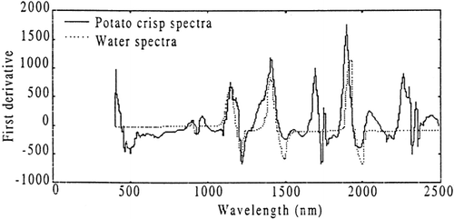
Before discussing the results of the predictor selection search heuristics, the general potato crisp spectra are compared with water. The shape of the potato crisp spectra is dependent on several different factors, including composition of the potato crisp and physical shape.

As 4 60% of the mass of the potato crisp samples comprises of water, a large portion of the absorption is due to hydroxyl bonding. The main absorption bands in water, located at 970, 1190, 1450 and 1940 nm (Petty and Curcio, 1951) are clearly visible in the water spectra, peaks located at 972, 1201, 1458, 1964 nm show up corresponding to O-H bonding in the potato spectra (see Fig. 3). This shows that a large amount of the spectral characteristics are due to O-H bonding.

Figure 3. Comparison of potato crisps spectra to water.

Full Spectrum Modeling

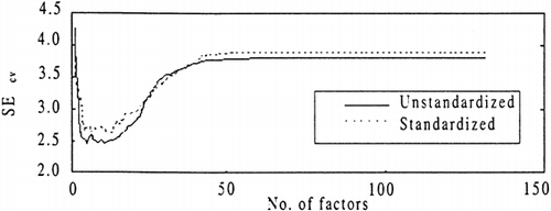
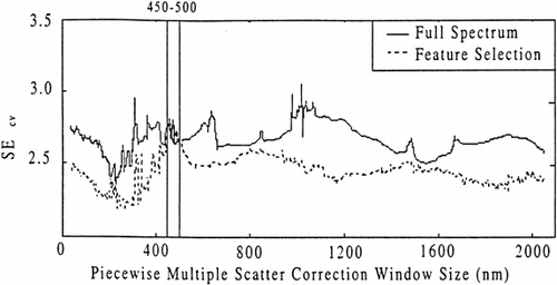
Full spectrum PLS results, shown in Figure 4, indicates the PLS models generated from unstandardized, MSC preprocessed data have lower cross validated errors and a smaller number of factors (9, as opposed to 19), than models obtained using standardized MSC preprocessed data. The overall minimum error in the standardized data is a SM_cv value of 2.66 corresponding to the third minimum at 19 factors. In contrast the minimum SM_cv value of 2.45 for the unstandardized data coincided with the first local minimum at 9 factors. This illustrates the danger in selecting the first minima as optimal without considering other local minima. Using this value for the optimum number of factors, the PMSC window size is varied between 20 and 2100 nm. The optimal window size is found to be located at 226 nm, shown in Figure 5. The improvement in SM_cv is a 6% percentage difference (Table 1), using PMSC over the MSC processed data with full spectrum modeling.

Figure 4. Comparison of standardized and unstandardized full spectrum model.

Figure 5. SE_cv vs. PMSC window size for feature selection and full spectrum methods.

Table 1. Search Heuristics Mean and Median SE_cv Values

Model	PMSC Window Size	SEcv (MSC)	SEcv (PMSC)	No. of Factors
GA	250	–	1.930 (median)	23
Hill climb	260	1.976 (median)	1.939 (median)	23
GA	250	–	1.9171 (mean)	23
Hill climb	260	1.986 (mean)	1.9366 (mean)	23
Feature selection	260	2.39	2.222	23
Full spectrum	226	2.45	2.353	9
Full spectrum (scaled)	–	2.66	–	19

Feature Selection Results

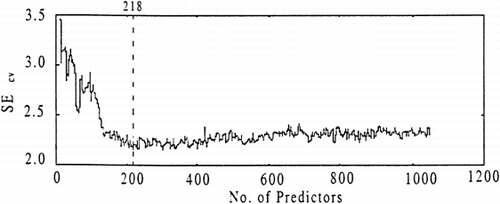
The feature selection method produced a minimum SM_cv at 218 predictors (see Fig. 6). The optimal number of factors that corresponded to this value is 23. The plot of SE_cv vs. PMSC window size (shown in Fig. 5) exhibits a trend of lower SE_cv values for feature selection models compared to the full spectrum model. All the SE_cv values, except those in the region of 450 nm to 500 nm, were lower. The optimal feature selection model was found to correspond to a PMSC window size of 260 nm. The improvement over the optimum full spectrum PMSC model is a 5.5% percentage difference and the improvement over the feature selection model with MSC is a 7.5% percentage difference (see Table 1).

Figure 6. SE_cv vs. number of wave length predictors using feature selection.

Hill Climbing and Genetic Algorithm Results

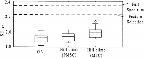
The box plot (Fig. 7) shows the SE_cv values of the hill climbing and GA methods. A total of 90 different runs are represented in the box plot, 30 for each of the hill climb and GA methods, each run had different randomly selected starting combinations. Each box in the plot encloses 50% of the SE_cv values, with the top and bottom of the box representing upper and lower quartiles. The lines protruding from the box indicate values that fall within acceptable range. Any point outside this range is indicated with a (o) and is termed as an outlier. These are mathematically defined as points which lie more than 1.5 times the interquartile range, above or below the upper or lower quartiles. The optimum model found in this investigation, is a SE_cv value of 1.82 in the GA box plot. This represents a 23% percentage difference improvement over the full spectrum model with PMSC and an 18% percentage difference improvement over the feature selection method with PMSC. The hill climb algorithm using PMSC produced a median SE_cv value of 1.939. This was of similar value to the median SE_cv value produced by the GA (1.930). A feature of the box plot worth mentioning is none of the SE_cv values in the hill climbing and GA plots were higher than the SE_cv values for the feature selection and full spectrum methods.

Figure 7. Box plot of SE_cv vs. different search heuristics with different starting combinations.

Using the mean SE_cv values for the GA and hill climbing methods (rows 3,4 table 1), the percentage difference in means was calculated. The performance increase obtained by the hill climbing algorithm with PMSC over hill climbing with MSC is a 3% percentage difference, the improvement over feature selection with PMSC is a 15% percentage difference and the improvement over the full spectrum method is a 22% percentage difference. The GA produced a 16% percentage difference improvement over feature selection with PMSC, a 23% percentage difference improvement over the optimum full spectrum model and the improvement over hill climbing with PMSC is a 1% percentage difference.

The significance of the percentage difference in mean was tested using statistical T-tests at the 95% significance level. Where both data sets have different variances the Welch statistic is used to estimate the pooled standard deviation (Wild and Seber, 2000), for use in calculation of the T-test statistic. Table 2 shows the T-test statistics for the GA and Table 3 shows the T-test statistics for the hill climb algorithm with PMSC. All the percentage differences in mean were judged significant at the 95% significance level, however the difference in means between the GA vs. hill climb with PMSC and the hill climb with PMSC vs. hill climb with MSC, would not be judged significant if the criteria had been a 97.5% significance level (denoted ‘*’ Tables 2-3.

Table 2. Significance Test Results of GA (mean SE_cv ) vs. Other Heuristics

Variable	N	SEcv	Std.	T-value	P-value
*Hill climb (PMSC)	30	1.9366	0.0529 (pooled)	− 2.05	0.049
Feature selection (PMSC)	1	2.222	0.520	− 32.11	0.000
Full spectrum (PMSC)	1	2.45	0.520	− 56.12	0.000

Table 3. Significance Test Results of Hill Climb with PMSC (mean SE_cv ) vs. Other Heuristics

Variable	N	SEcv	Std.	T-value	P-value
*Hill climb (MSC)	30	1.9568	0.0541 (pooled)	− 2.05	0.049
Feature selection (PMSC)	1	2.222	0.05377	− 29.07	0.000
Full spectrum (PMSC)	1	2.45	0.05377	− 52.29	0.000

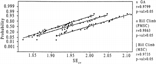
The results drawn from the T-tests are based on the assumption that the data is approximated by the normal distribution. The appropriateness of this assumption determines whether the error estimate is valid. This is an important consideration, given that the T-values are based on the computed mean square. To evaluate these issues the Wilk Shapiro W-test was used to test for normality (Shapiro et al., 1968). Figure 8 shows a plot of the normalized probability vs. SE_cv . Using the Wilk Shapiro test a high correlation between the SE_cv and the normalized probability provides strong evidence of a normal relationship. The correlation statistics were 0.9799, 0.9863 and 0.9735 respectively for the GA, hill climb with PMSC and the hill climb with MSC. The P-values corresponding to the correlation coefficients were all greater than 5% (0.05), providing no evidence against a normality hypothesis.

Figure 8. Normalized probability vs. the SE_cv for GA and hill climbing search heuristics.

Piecewise Multiple Scatter Correction Window Size Selection Results

The plot of the SE_cv vs. the optimal PMSC window size (Fig. 9) for the GA and the hill climb with different starting combinations shows a spread of optimal PMSC window values from 45 nm to 490 nm. The plot also shows a minima located at 250 nm. Both search heuristics appear to converge at this minima, however the GA appears to have lower SE_cv values, also illustrated by the box plot (Fig. 7). As one moves away from the minima, it is evident that the SE_cv value increases with a change in PMSC window size. This suggests that there is a relationship between the combinations of predictors and the PMSC window size, however a quantitative study of this relationship is outside the scope of the investigation.

Figure 9. SE_cv vs. optimal PMSC window size for hill climbing and GA with random initial selections of predictors.

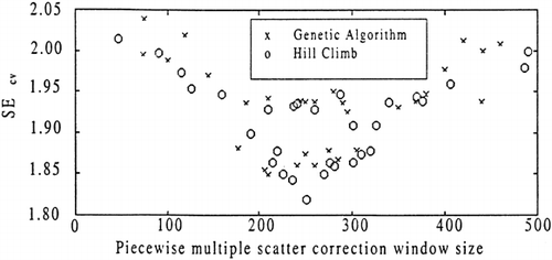
Absorption bands in the NIR are known to have broad spectral features, with widths of absorption bands being near 100 nm (Wilson, 1994). To reduce loss of information associated with additive and multiplicative effects resulting from scattering of the spectra, the PMSC window size should be larger than the absorption bandwidth. Our results are consistent with this. The most prominent O-H absorption bands, located at 970, 1190, 1450 and 1940 nm, correspond to a minimum distance between spectral overtones of 220 nm. An optimal window size of 250 nm may correspond to the size required to isolate the known O-H absorption bands.

CONCLUSIONS AND RECOMMENDATIONS

The GA architecture provides significant performance improvements over the methods of full spectrum modeling, feature selection and hill climbing, in the task of optimal spectral predictor and PMSC window size selection. The GA architecture described provides a single step optimization approach by simultaneously identifying both optimal PMSC window size and wavelength predictors. All the other architectures described identify optimal spectral wavelength predictors followed by PMSC window size. This research suggests that there is an inter-relationship between the wavelength predictors selected and PMSC window size. It is concluded that the GA architecture described, by simultaneously selecting both PMSC window size and wavelength predictors provides a degree of invariance to this inter-relationship and thus has advantages over the other methods discussed in this paper.

The prediction of potato crisp moisture, the use of PMSC leads to improved results over MSC. It is thus recommended that this form of pre-processing be used to correct for inherent shape curvatures and contours in non-destructive testing of potato crisps. The recommended method for selecting optimal combinations of spectral predictors and PMSC window size is the GA with the architecture described in this paper.

The moisture content of potato crisp can be determined to an accuracy of 1.82 SE_cv using the GA architecture. This suggests a high enough accuracy is possible for an automated inspection system, however the dataset contained two different varieties of potatoes that were treated without differentiation, to form a single dataset. At present the effect of different potato varieties on the results is still under investigation. In the future it is intended to focus on the methods of automated potato variety classification for an automated classification and properties determination system.

Acknowledgments

REFERENCES

- Batten , G. , Flinn , P. , Welsh , L. and Blake , A. , eds. 1997 . Leaping Ahead with Near Infrared Spectroscopy, Chapter, Piece-wise Multiple Scatter Correction PMSC 95 – 98 . New York : Wiley .
- Chambers , L. 1995 . Practical Handbook of Genetic Algorithms Boca Roton, Florida : CRC Press .
- Frenich , A. G. , Jouan-Rimbaud , D. , Massart , D. L. , Kuttatharmmakul , S. , Martinez , G. M. and Vidal , J. 1995 . Wavelength Selection Method for Multicomponent Spectrophotometric Determinations Using Partial Least Squares Analysis . Analyst , 120 : 2787 – 2792 .
- Geladi , P. , MacDougall , D. and Martens , H. 1985 . Linearization and Scatter Correction for Near Infrared Reflectance of Meat . Applied Spectroscopy , 39 ( 5 ) : 491 – 500 .
- Guchardi , R. , Filho , P. , Poppi , R. and Pasquni , C. 1998 . Determination of Ethanol and Methyl Tert-Butyl Ether Mtbe in Gasoline by NIR-AOTF Based Spectroscopy and Multiple Linear Regression with Variables Selected by Genetic Algorithm . Applied Spectroscopy , 55 ( 6 ) : 257 – 266 .
- Isaksson , T. and Kowalski , B. 1993 . Piece-Wise Multiplicative Scatter Correction (MSC) and Linearity in NIR Spectroscopy . Applied Spectroscopy , 42 ( 7 ) : 1273 – 1284 .
- 1993 . “ Moisture Systems Corporation ” . In Report: December Applications Newsletter Hopkinton, , MA, USA : Moisture Systems Corporation . 117 South Street
- Nollet , L. 1996 . Handbook of Food Analysis 72 – 73 . New York : Marcel Dekker . ISBN 0-8247-9682-9
- Osborne , S. D. , Jordan , R. B. and Kunnemeyer , R. 1997 . Method of Wavelength Selection for Partial Least Squares . Analyst , 122 : 1531 – 1537 .
- Petty , C. and Curcio , J. 1951 . The Near Infrared Absorption Spectra of Liquid Water . Journal of the Optical Society of America , 41 ( 5 ) : 301 – 306 .
- Shaffer , R. 1996 . Optimization Methods for the Analysis of Infrared Spectral and Interferogram Data , Ph.d. Thesis Ohio : Ohio University .
- Shapiro , S. , Wilk , M. and Chen , H. 1968 . A Comparative Study of Various Tests for Normality . Journal of the American Statististical Association , 63 : 1343 – 1372 .
- Stone , M. 1974 . Cross-Validatory Choice and Assessment of Statistical Predictions . Journal of the Royal Statistical Society , Series B : 111 – 133 .
- Van den Broek , W. H. , Wienke , D. , Melssen , W. J. and Buydens , L. M. 1997 . Optimal Wavelength Range Selection by a Genetic Algorithm for Discrimination Purposes in Spectroscopic Infrared Imaging . Applied Spectroscopy , 51 ( 8 ) : 1210 – 1217 .
- Wild , C. and Seber , G. 2000 . Chance Encounters 339 – 441 . New York : Wiley .
- Wilson , R. 1994 . Spectroscopic Techniques for Food Analysis 100 – 115 . New York : VCH Publishers .
- Withers , B. 1998 . “ Report: Possible Methods to Reduce Browning of Potato Crisps ” . In Department of Food Technology Palmerston North, , New Zealand : Mssey University .
- Wold , H. 1966 . Multivariate Analysis 391 – 410 . New York : Academic Press .