A mixed effects model to estimate timing and intensity of pubertal growth from height and secondary sexual characteristics

Abstract

Aim: To estimate and compare pubertal growth timing and intensity in height, Tanner stage markers and testis volume.

Subjects and methods: Data on height, genital stage, breast stage and pubic hair stage, testis volume and menarche in 103 boys and 74 girls from the Edinburgh Longitudinal Growth Study were analysed. The SITAR model for height and a novel mixed effects logistic model for Tanner stage and testis volume provided estimates of peak velocity (PV, intensity) and age at peak velocity (APV, timing), both overall (from fixed effects) and for individuals (random effects).

Results: Based on the six markers, mean APV was 13.0–14.0 years in boys and 12.0–13.1 years in girls, with between-subject standard deviations of ∼1 year. PV for height was 8–9 cm/year by sex and for testis volume 6 ml/year, while Tanner stage increased by 1.2–1.8 stages per year at its peak. The correlations across markers for APV were 0.6–0.8 for boys and 0.8–0.92 for girls, very significantly higher for girls (p = 0.005). Correlations for PV were lower, −0.2–0.6.

Conclusions: The mixed effects models perform well in estimating timing and intensity in individuals across several puberty markers. Age at peak velocity correlates highly across markers, but peak velocity less so.

• Height
• mixed effect model
• puberty
• Tanner stage
• velocity

Introduction

There is now considerable interest in the life course, particularly in the idea that patterns of child growth may influence the risk of adverse adult outcomes such as cardiovascular disease, diabetes or hypertension (Kuh & Ben-Shlomo, 2004). Puberty is a period of intense hormonal activity and rapid growth, of which the most striking feature is the spurt in height, whose intensity in individuals is measured by peak height velocity (PHV) and its timing by age at PHV (APHV).

Mean PHV is ∼10 cm/year in boys and 9 cm/year in girls, while mean APHV is ∼13.5 and 11.5 years by sex (Tanner et al., 1966). However, there is considerable variability in the intensity and timing of the spurt from one child to another, with standard deviations of ∼1 cm/year for PHV and 1 year for APHV (Tanner et al., 1966). PHV and APHV can be estimated from longitudinal height data by fitting parametric growth curves such as Preece-Baines (Preece & Baines, 1978) or JPA2 (Jolicoeur et al., 1992) or cubic spline curves (Cole et al., 2008) or, more recently, with the SITAR method of growth curve analysis (SuperImposition by Translation And Rotation) (Cole et al., 2010). SITAR is a shape invariant model consisting of a mean cubic spline curve and subject-specific random effects. Together these effects provide estimates of the timing and intensity of pubertal height growth in individuals.

In addition to height, several secondary sexual characteristics mark the individual’s passage through puberty: the ‘Tanner’ developmental stages of genitalia in boys, breasts in girls and pubic hair in both sexes (Marshall & Tanner, 1969, 1970), plus testis volume in boys and menarche in girls. As with height, the timing of these events in individuals is very variable. However, estimating the mean age of a given developmental stage is complicated by the fact that the data are unobservable—the age that a child enters or leaves a given stage cannot be observed directly.

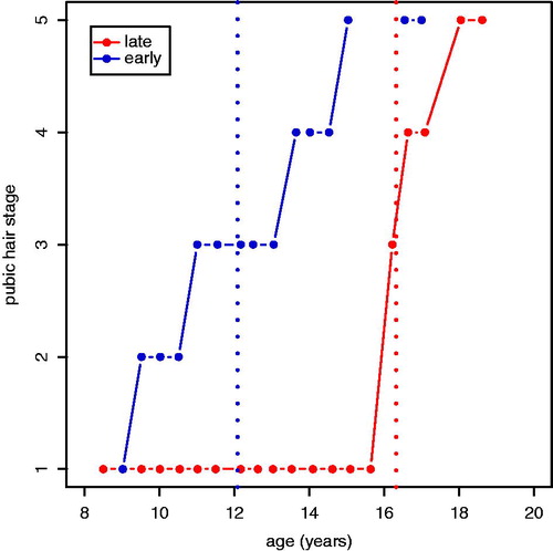
Marshall & Tanner (1969, 1970) estimated the mean ages for each stage using the method of Swan (1969) and for intensity they measured the time period between selected pairs of stages, e.g. from stage 2–5. A recent paper by Gasser et al. (2013) uses similar methodology. To illustrate variation in timing and intensity, Figure 1 shows serial measures of Tanner pubic hair stage plotted against age in two selected boys. The first boy takes 6 years, from age 9–15, to pass from stage 1 to stage 5, a rate of four stages in 6 years. In contrast, the second boy proceeds from stage 1 to stage 5 in only 3 years, from age 15–18. The timing of the passage from stage 1 to stage 5 is summarized by the mean age in stage 3. This is marked by vertical lines in Figure 1, so the first boy’s timing is 12 years and his intensity is 4/6 or 0.67 stages per year, while for the second his timing is 16.5 years and his intensity 4/3 or 1.33 stages per year, twice as fast.

Figure 1. Pubic hair stage plotted against age in two boys, selected to show early vs late pubertal timing and low vs high pubertal intensity. The vertical lines indicate age at peak velocity.

A weakness with previous approaches to the estimation of pubertal timing and intensity is that they have focused on individual stages or pairs of stages. If there was a way to make use of all the available stage measurements per individual it would increase efficiency. The aim of this paper is to describe a toolbox of statistical methods, including SITAR, to do just that for height, Tanner stages, testis volume and menarche. The methods efficiently estimate peak velocity (PV) and age at peak velocity (APV) for each marker, in individual subjects and overall, and they are illustrated using data from the Edinburgh Growth Study.

Methods

The Edinburgh Longitudinal Growth Study was set up in 1972 by Dr Shirley Ratcliffe of the MRC Human Genetics Unit, Edinburgh, UK, where 103 boys and 74 girls acted as the controls in a study of growth and cytogenetic abnormality (Ratcliffe et al., 1986, 1991; Butler et al., 1989). Measurements of height from birth and from age 5 Tanner stages of pubic hair (both sexes), breast development (girls) and genital development and testis volume by Prader orchidometer (boys) were obtained every quarter- or half-year until 20 years. Menarche (girls) was recorded as the month of age when menses first occurred.

The aim here is to fit growth curve models for each of the pubertal markers by sex, providing subject-specific measures of pubertal timing and intensity. For height this is achieved with the SITAR model (Cole et al., 2010), restricted to measurements over age 5 to match the pubertal markers: where y_it is height in the ith subject at age t; α_i, β_i and γ_i are random effects for subject i and h(.) is a cubic spline curve. Corresponding fixed effects α₀, β₀ and γ₀ are also fitted. The residual errors and random effects are assumed to be normally distributed with mean zero and statistically independent. The meanings of α_i, β_i and γ_i are as follows:

• α_i is mean height in subject i, expressed relative to overall mean height and measured in units of centimetres. Called size, it corresponds to the intercept in a random intercept model and geometrically it equates to a shift up or down of the mean curve on the height scale.

• β_i is the tempo or timing of PHV in subject i, their APHV expressed relative to mean APHV in units of years. It corresponds to a shift left or right of the mean curve on the age scale.

• γ_i is a measure of mean velocity or intensity in subject i, their PHV relative to mean PHV. Geometrically it corresponds to a stretching or shrinking of the age scale, which has the effect of decreasing or increasing the slope, i.e. mean velocity, of the curve. It is measured in fractional units and, multiplied by 100, it can be viewed as a percentage difference from mean PHV. The effect on velocity applies across the age range, so it applies to PHV and velocity at other ages and it has an inverse effect on the duration of puberty in the individual.

Thus, in general terms α is a measure of size, while β and γ are measures of, respectively, timing and intensity of pubertal growth. The function h(.) in equation (1) is fitted with a natural cubic regression spline, with degrees of freedom selected to minimize the Bayesian Information Criterion (BIC) (Schwarz, 1978).

For Tanner-stage-based sexual characteristics and testis volume, a longitudinal mixed model is needed to quantify timing and intensity and an obvious solution would be to use SITAR. However, simpler models are possible, as the corresponding growth curves are not as complex as the height curve. Consider the logistic model which allows y_t to take values between the asymptotes 0 and 1, such that when , when and when . Thus, β represents the timing of the process, the age when the velocity of y_t is at its peak. The model can be applied either to binary 0/1 variables or to continuous variables bounded by 0 and 1.

Tanner stage plotted against age follows the logistic form of equation (2), with stage 1 as the lower asymptote and stage 5 the upper asymptote. So, equation (2) can be extended as follows, using the same transformed age notation as for SITAR (equation 1):

Here, when t is small and when t is large; the random effects β_i and γ_i are measures of timing and intensity, analogous to those for height (equation 1), where β_i is the individual’s mean age in stage 3, the age when stage is changing most rapidly, and γ_i indicates the relative rate of change of stage at this age, i.e. peak velocity.

The same logistic form can also be applied to mean testis volume, except that here the lower asymptote (corresponding to childhood) is ∼1 ml and the upper asymptote (adulthood) is 20–25 ml. So, for mean testis volume, equation (3) is extended as follows:

There are now four subject-specific random effects, α_i, β_i, γ_i and δ_i, where α_i is adult testis volume, δ_i is child testis volume and β_i and γ_i are measures of timing and intensity of the testis volume growth spurt equivalent to those in equations (1) and (3). In particular, when then , the mean of child and adult testis volume, at the age when testis volume is increasing most rapidly, while γ_i measures the relative rate of rise of the logistic curve. Equation (4) is modified from a model proposed by Gasser et al. (2013).

For completeness the Tanner stage and testis volume curves are also fitted using SITAR (equation 1) and the fit relative to the logistic models (equations 3 and 4) assessed using BIC. All the mixed effects models are fitted in the statistical language R (R Core Team, 2012) using the nlme package (Pinheiro et al., 2012), from which a dedicated sitar library has been developed. The random effects are assumed to have an unstructured covariance matrix and the fixed effects define the population mean curves. For SITAR the starting values for the spline curve coefficients (including α₀) come from the curve , with the data treated cross-sectionally. This model is equivalent to equation (1), without the random effects and with the fixed effect coefficients absorbed into the spline coefficients, and it provides the fixed effects residual SD. The starting value for β₀ is set to mean APHV from this same curve and that for γ₀ is set to zero. For testis volume, equation (4) turns out to fit better with δ as a fixed effect rather than a random effect.

Equivalent fixed effects logistic models, omitting the random effects, are fitted using the nls package in R. The impact of adding the random effects to these models is quantified as the extra variance explained, defined as where σ_m and σ_f are the residual standard deviations from the mixed and fixed models, respectively.

Menarche, unlike the other pubertal markers, is a binary 0/1 variable. As such its timing β_i in individuals is their age at menarche relative to mean age at menarche. However, there is no equivalent measure of intensity γ_i as there is only one event.

Taken together, equations (1), (3) and (4) provide estimates of timing and intensity for height, Tanner breast, genital and pubic hair stages, plus testis volume and menarche (timing only). This allows the mean timings and intensities to be compared for the different markers and also allows the individual subject values, based on the random effects, to be correlated across markers. For SITAR the timing and intensity are estimated by differentiating the spline curve to obtain the velocity curve and reading off the peak velocity and the age when it occurs. For the logistic models (equations 3 and 4), β₀ estimates timing explicitly, i.e. mean APV in units of years and its standard deviation (SD) is obtained as the SD of the random effect β_i. The mean intensity, i.e. PV, is derived as in equation (3) and in equation (4). The SD of PV is obtained as the SD of γ_i multiplied by mean PV. The peak velocities are in measurement units per year. For menarche, the mean and SD of APV are derived from the individual menarcheal ages. The correlations between timing and intensity are those for the random effects β_i and γ_i in each model.

For each sex the six correlations between the four markers are averaged by treating the correlation matrix as compound symmetric. The second and subsequent eigenvalues of this matrix are equal to , where r is the mean correlation, and the logarithm of the eigenvalue is asymptotically normally distributed with variance , where n is the sample size (Jolliffe, 2002). So to compare the mean correlations by sex has variance , where the subscripts refer to the two sexes.

The outcome of each analysis is a population mean curve based on fixed effects and a set of subject-specific random effects. Thus, there is just one fitted curve, where the random effects are set to zero, and the random effects transform the mean curve to model individual subject curves. This is the basis for a shape invariant model. For presentation purposes this process is reversed here, using the random effects to back-transform the data for the individual growth curves. If the fit is adequate these curves will then be effectively superimposed on the mean curve, providing a visual demonstration both of the shape of the mean curve and the overall goodness of fit. In practice this is achieved by plotting each outcome measure adjusted for size α_i, (which are, respectively, in equation (1), in equation (3) (no adjustment needed) and in equation (4)) against age adjusted for timing β_i and intensity γ_i, i.e. .

Results

For ages over 5 years there were 2469/1561 heights in 103/74 boys/girls (Table 1). Individual height growth curves from 5 years to adult are shown in Figure 2(a) and (b) by sex. SITAR models of height vs age were fitted for each sex using spline curves with 9/7 df, leading to residual standard deviations of 0.9/0.7 cm each, explaining 98.4% of the variance compared to the fixed effects models.

Figure 2. Individual height growth curves for (a) 103 boys and (b) 74 girls. The same growth curves after SITAR adjustment for size, timing and intensity are shown in (c) boys and (d) girls, where the curves are superimposed, and the population mean curve is shown in white. The vertical lines indicate mean age at peak height velocity.

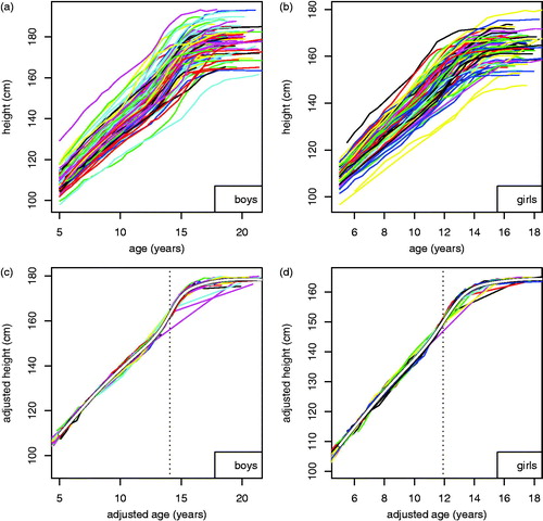
Table 1. Summary statistics for timing and intensity of puberty.

			Age at peak velocity (years)		Peak velocity (units/year)		Residual SD (units)
Sex	Marker	n subjects/ measures	Mean (SE)	SD	Mean	SD	Fixed effects model	Randomeffects model	Variance explained* (%)	Correlation (APV-PV)
Boys	Height (cm)	103/2469	14.1 (0.13)	1.03	9.7	0.83	6.9	0.89	98.4	−0.65
	Genital stage	98/1383	13.0 (0.08)	0.80	1.2	0.35	0.60	0.31	73.8	−0.25
	Pubic hair stage	98/1319	13.7 (0.10)	0.94	1.7	0.68	0.72	0.26	86.4	0.07
	Testis volume (ml)	101/1409	13.3 (0.12)	1.13	6.3	2.7	3.4	1.08	89.8	−0.71
Girls	Height (cm)	74/1561	11.9 (0.20)	1.01	7.6	0.91	6.0	0.76	98.4	−0.78
	Breast stage	74/961	12.0 (0.13)	1.09	1.5	0.39	0.75	0.29	84.8	0.20
	Pubic hair stage	74/825	12.6 (0.12)	0.97	1.8	0.68	0.74	0.25	88.8	−0.06
	Menarche	70/70	13.1 (0.15)	1.21	–	–	–	–	–	–

*Compared to fixed effects model.

The individual curves after SITAR adjustment are shown in Figure 2(c) and (d) by sex, with the individual curves shown in colour, the mean fitted curves in white and the mean ages at peak height velocity highlighted as vertical dotted lines. The SITAR adjustment causes the individual curves to appear superimposed on the mean curve. The few apparently discrepant curves after 12 years are due to missing data during the growth spurt.

The Tanner stage markers were fitted both to the SITAR model (equation 1) and the logistic model (equation 3). For breast stage, the BIC for the SITAR model with 3 df was 18 units larger than for the logistic model, while none of the other SITAR models converged. Thus, the results here are restricted to the logistic models, as summarized in Table 1. The extra variance explained by adding the random effects to the fixed effects models ranged from 74–89%.

Figure 3, like Figure 2, shows patterns for the Tanner stage markers, based on 98/74 boys/girls: (a) genital stage and (c) pubic hair stage in boys, (b) breast stage and (d) pubic hair stage in girls. In each graph the unadjusted curves are shown in the background (in grey), with the same curves adjusted for subject timing and intensity random effects from equation (3) superimposed (in black). Also superimposed is the mean logistic curve (in white) and a dotted vertical line indicating mean APV for the marker. The residual SDs about the mean curves vary between 0.25–0.31 stage units (Table 1) and the residuals are close to normally distributed (not shown).

Figure 3. Individual growth curves for (a) genital stage and (c) pubic hair stage in 98 boys and (b) breast stage and (d) pubic hair stage in 74 girls. The raw curves appear in grey, while the same curves adjusted for individuals’ timing and intensity with equation (3) are superimposed in black. The population mean logistic curves are in white and the vertical lines indicate mean age at peak velocity.

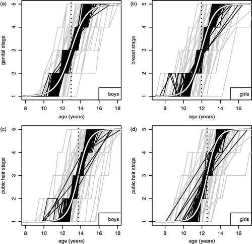
The effect of adjusting for timing and intensity in Figure 3 is to cluster the curves, allowing the mean logistic patterns to emerge. The stepped appearance arises because, although individuals usually progress from one stage to the next during puberty, they remain in the same stage for between a fifth and a half of the time periods (depending on the marker and ignoring intervals spent in stages 1 or 5). The clustering is less tight than for height (Figure 2) and the fit is relatively poor at the start and end of puberty, but it does allow the data to be combined to estimate mean PV and APV. Referring back to Figure 1, note that the vertical lines there mark the subject-specific APVs for pubic hair, which are close to the mean ages in stage 3. This demonstrates that, in general, APV for the Tanner stages corresponds to the mean age in stage 3.

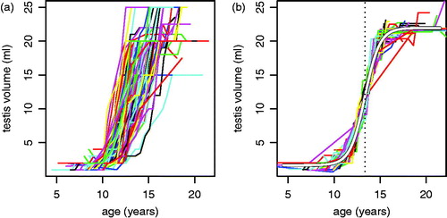
Testis volume was fitted to the SITAR model (equation 1) with 5 df and the logistic model (equation 4) and the logistic fitted appreciably better (relative BIC −238). Figure 4 shows testis volume growth curves based on equation (4) for 101 boys, unadjusted (Figure 4a) and adjusted for timing, intensity and adult testis volume (Figure 4b). Here again the adjustment causes the individual curves to cluster around the mean curve, with 90% of the variance explained (Table 1). The residual SD is 1.1 ml and the estimated child and adult asymptotes are δ₀ = 1.7, SE 0.7 ml and α₀ = 21.9, SE 0.3 ml, respectively.

Figure 4. Individual testis volume growth curves for 101 boys, (a) raw and (b) adjusted for timing and intensity with equation (4). In (b) the population mean curve is shown in white and the vertical line indicates mean age at peak testis volume velocity.

Table 1 summarizes the estimates of timing (APV) and intensity (PV) in the puberty markers by sex. Mean age at peak velocity is 13–14 years in boys and 12–13 years in girls, depending on the marker, while the SD for APV is 0.8–1.1 years. The PV for height is 9.7 cm/year in boys and 7.6 cm/year in girls, with SDs ∼0.9 cm/year. PV for testis volume is 6.3 (SD = 2.7) ml/year and for the four Tanner stages PV is between 1.2–1.8 stages per year. (The PVs in Figure 1 of 0.67 and 1.33 are smaller but are not directly comparable, as they cover stage 1 to stage 5, whereas the PVs in Table 1 are instantaneous velocities in stage 3.) The SDs of PV are appreciably greater and the percentage of variance explained rather smaller for the Tanner stages than for height or testis volume, despite having smaller means, indicating greater measurement error.

The correlations between APV and PV are ∼−0.7 for height and testis volume, but much closer to zero for the Tanner stages. Thus, for height and testis volume early maturers tend to have a higher peak velocity, suggesting that their individual body clocks are running faster and they pass through puberty more quickly than later maturers.

Figures 5 and 6 show scatterplot matrices of timing and intensity for the four markers by sex, with the correlations superimposed and their font size scaled appropriately. The correlations between markers for pubertal timing (upper triangle) are generally high, ∼0.6–0.8 in boys and 0.8–0.9 in girls, but very significantly higher in girls (mean correlations 0.76 and 0.87 respectively, p = 0.005). For intensity the correlations are much lower (lower triangle), 0.1–0.6 in boys and −0.2–0.2 in girls, with the girls’ correlations close to zero (sex difference, p = 0.2).

Figure 5. Scatterplot matrix for boys showing the correlations between four pubertal markers for timing (upper triangle) and intensity (lower triangle). The correlation values are included, with the font size scaled to reflect the value.

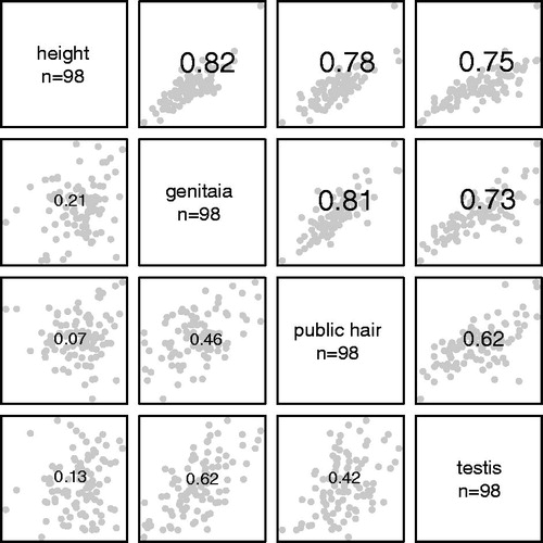
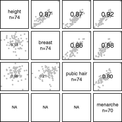
Figure 6. Scatterplot matrix for girls showing the correlations between four pubertal markers for timing (upper triangle) and intensity (lower triangle). The correlation values are included, with the font size scaled to reflect the value.

Discussion

The process of pubertal growth and development can be monitored by four distinct markers in each sex; height, genitalia/breast, pubic hair and testis volume/menarche. The results of this analysis, based on longitudinal data from the Edinburgh Growth Study, show how closely linked the markers are in terms of their timing (age at peak velocity) and intensity (peak velocity). The statistical methods developed here allow timing and intensity to be efficiently estimated for each marker and then compared across markers within individuals.

The strength of this approach is most obvious with the Tanner stage markers. Usually the timings of breast, genital and pubic hair stages are based on the age of onset of individual stages, e.g. breast stage 2, while intensity is measured by the time elapsed between pairs of stages, e.g. stages 2–5 (Marshall & Tanner, 1969, 1970; Gasser et al., 2013). Here, however, the whole ‘growth curve’ for the marker is modelled, using all the available longitudinal data, which results in efficient estimates of both the mean age at peak velocity (effectively the mean age in stage 3) and the mean peak velocity, the rate of change of the stage. Note that this is the mean age in stage 3, not the mean age of onset of stage 3, which is what is usually estimated with cross-sectional data. In addition, testis volume is modelled the same way, using a variant (equation 4) of the model proposed by Gasser et al. (2013), but fitted as a mixed effects model rather than to individuals.

The Tanner stage measurement scale is somewhat artificial, with peak velocity in units of stages of per year and age at peak velocity corresponding to mean age in stage 3. Yet the logistic curve with normal errors provides a reasonable fit to the longitudinal stage data (see Table 1 and Figure 3) and the definitions of peak velocity and age at peak velocity lead from the units of measurement.

Fitting the logistic model (equation 3) with and without random effects gave very similar estimates for the mean age at peak velocity β, all within 0.1 years (data not shown). This suggests a way of estimating the mean timing of puberty in cross-sectional growth studies, by fitting the fixed effects logistic model (equation 3) to Tanner stage markers. The resulting ages can be compared to the age at peak height ‘velocity’ based on the first derivative of the cross-sectional mean height curve, which is an unbiased estimate of the underlying longitudinally-based age at peak velocity (Cole et al., 2008).

Figures 2–4 show that the models adjusted for individual variation in timing and intensity fit the data well. The SITAR models, for example, explain 98.4% of the variability in height and the logistic models between 74–90%. The fixed effects provide efficient estimates of the mean timing and intensity of the growth spurt, while the random effects show how individuals vary in these respects. Despite the fact that the Tanner stage data are granular, on the integer scale 1–5, the residuals from the models are consistently close to normal.

The SITAR growth curve model’s three random effects were called size, tempo and velocity when first published (Cole et al., 2010). The size effect is not relevant for this study, being a reflection of mean height over time in the individual and for this reason it has not been highlighted. The tempo and velocity effects are just different names for timing and intensity, as used here.

On average the first pubertal marker to reach peak velocity in boys is genital stage (at age 13.0 years, Table 1), closely followed by testis volume, pubic hair stage and then height. In girls the sequence is height (11.9 years) and breast stage (12.0 years), followed by pubic hair then menarche (13.1 years). The standard deviations of these mean timings are all close to 1 year (Table 1). This sequence is similar to those seen in other studies (Marshall & Tanner, 1970; Gasser et al., 2013).

Peak height velocity approaches 10 cm/year for boys and 8 cm/year for girls, slightly lower than Tanner’s figures for instantaneous velocity (Tanner et al., 1966). Among the Tanner markers, genital stage proceeds at the slowest rate (mean peak velocity 1.2 stages/year), with breast stage next (1.5) and pubic hair fastest (1.7 and 1.8 by sex). Thus, the progression through four stages, from stage 1 to 5, takes longest for genitalia and shortest for pubic hair. For comparison the mean PV for testis volume is 6.3 ml/year, with the change in volume from child to adult averaging ∼20 ml. So testis volume PV can be re-scaled crudely to Tanner stage units, based on the ‘distance’ travelled, to give PV = 6.3/20 × 4 = 1.3 stages/year, close to that for genital stage. This is reassuring, as genitalia and testes ought to be developing in tandem.

For height in both sexes and testis volume in boys there is a strong inverse correlation of −0.7 between APV and PV, meaning that early maturers have a higher PV and progress through puberty more quickly than later maturers. This implies that the underlying passage of time is multiplicative rather than additive, with an elastic age scale where early puberty corresponds to shrinking the scale and late puberty to stretching it. This in turn makes the growth curve steeper or shallower depending on the timing, hence generating the negative correlation between APV and PV.

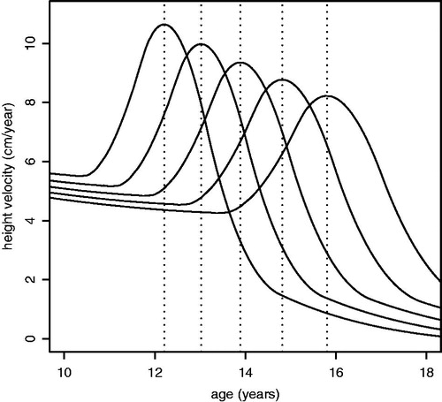
There is empirical support for this idea. Refitting the SITAR height models using log age rather than age improves the fit by 185 and 190 units of deviance for boys and girls, respectively, and the corresponding correlations between APV and PV of +0.3 and −0.2 are appreciably smaller than before. Using log age also improved the fit for Christ’s Hospital School boys (Cole et al., 2010). Velocity curves based on the multiplicative model are seen in Figure 7 for five hypothetical boys, closely matching the famous Figure 1 from Tanner et al. (1966). This confirms that the age effect is closer to multiplicative than additive.

Figure 7. Predicted height velocity curves for boys from a SITAR model of height vs log age, where the tempo random effect varies from −2 to +2 standard deviations.

There is little sign of a multiplicative age effect with the other markers, and particularly for girls, where the correlations between APV and PV are close to zero. This may reflect the greater measurement error of Tanner stage markers, coupled with possible inadequacy of the logistic model at the extremes, or it may hint at a more general truth that puberty as measured by secondary sexual characteristics is not accelerated in early maturers.

As to the correlations between markers, Figures 5 and 6 provide simple visual summaries for the two sexes. For girls the timing of peak velocity is quite tightly linked across markers, with correlations of 0.8 upwards, and between height and menarche it is as high as 0.92. For boys the correlations are very significantly lower, in the range 0.62–0.82, and there is little overlap with the girls’ values. For intensity the story is reversed, with higher correlations for boys than girls, although height intensity is uncorrelated with the other markers in either sex.

The main limitation of the study is the sample size, 103 boys and 74 girls, reflecting the effort required to set up and maintain such a study over 20 years. Other longitudinal growth studies are similarly modest in size—the 1st Zurich Longitudinal Growth Study for example had 120 boys and 112 girls (Gasser et al., 2013). It means that the confidence intervals around the correlations are relatively wide, but even so the sex difference in the size of correlations between markers is highly significant (p  = 0.005) and is probably genuine. The strength of the study is its demonstration that the unified modelling approach fits the data well, and it allows the individual patterns of pubertal growth to be concisely summarized. In addition the mixed effects model allows all individuals to be included in the analysis, whereas individually fitted models inevitably fail to fit in a few cases (Sandhu et al., 2006; Molinari et al., 2013).

In conclusion, a logistic growth model is proposed that efficiently models serial changes in Tanner stage and testis volume through puberty, and which allows the timing and intensity of the growth spurt to be documented for height and secondary sexual characteristics.

Declaration of interest

The authors report no conflicts of interest. The authors alone are responsible for the content and writing of the paper.

Acknowledgements

The authors dedicate the paper to Dr Shirley Ratcliffe, the inspiration behind the Edinburgh Growth Study, who died on 17 July 2013. The authors also thank the two reviewers for their useful comments, which improved the paper considerably. Dr Marco Geraci was helpful in developing the test to compare compound symmetric matrices. TJC was supported by Medical Research Council grant MR/J004839/1.

References

- Butler GE, Walker RF, Walker RV, Teague P, Riadfahmy D, Ratcliffe SG. 1989. Salivary testosterone levels and the progress of puberty in the normal boy. Clin Endocrinol 30:587–596
- Cole TJ, Cortina Borja M, Sandhu J, Kelly FP, Pan H. 2008. Nonlinear growth generates age changes in the moments of the frequency distribution: the example of height in puberty. Biostatistics 9:159–171
- Cole TJ, Donaldson MD, Ben-Shlomo Y. 2010. SITAR – a useful instrument for growth curve analysis. Int J Epidemiol 39:1558–1566
- Gasser T, Molinari L, Largo R. 2013. A comparison of pubertal maturity and growth. Ann Hum Biol 40:341–347
- Jolicoeur P, Pontier J, Abidi H. 1992. Asymptotic models for the longitudinal growth of human stature. Am J Hum Biol 4:461–468
- Jolliffe IT. 2002. Principal component analysis. New York, NY: Springer-Verlag
- Kuh D, Ben-Shlomo Y, editors. 2004. A life course approach to chronic disease epidemiology. 2nd ed. Oxford: Oxford University Press. p 473
- Marshall WA, Tanner JM. 1969. Variations in pattern of pubertal changes in girls. Arch Dis Child 44:291–303
- Marshall WA, Tanner JM. 1970. Variations in pattern of pubertal changes in boys. Arch Dis Child 45:13–23
- Molinari L, Gasser T, Largo R. 2013. A comparison of skeletal maturity and growth. Ann Hum Biol 40:333–340
- Pinheiro J, Bates D, DebRoy S, Sarkar D, R Core team. 2012. nlme: linear and nonlinear mixed effects models. R package version 3.1-105
- Preece MA, Baines MJ. 1978. A new family of mathematical models describing the human growth curve. Ann Hum Biol 5:1–24
- R Core Team. 2012. R: a language and environment for statistical computing. Vienna, Austria: R Foundation for Statistical Computing
- Ratcliffe SG, Butler GE, Jones M. 1991. Edinburgh study of growth and development of children with sex chromosome abnormalities IV. Birth Defects: Original Article Series 26:1–44
- Ratcliffe SG, Murray L, Teague P. 1986. Edinburgh study of growth and development of children with sex chromosome abnormalities III. Birth Defects: Original Article Series 22:73–118
- Sandhu J, Davey Smith G, Holly J, Cole TJ, Ben-Shlomo Y. 2006. Timing of puberty determines serum insulin-like growth factor-1 in late adulthood. JCEM 91:3150–3157
- Schwarz G. 1978. Estimating the dimension of a model. Ann Statist 6:461–464
- Swan AV. 1969. Computing maximum-likelihood estimates for parameters for normal distribution from grouped and censored data. Appl Stat 18:65–69
- Tanner JM, Whitehouse RH, Takaishi M. 1966. Standards from birth to maturity for height, weight, height velocity, and weight veloc British children, 1965 Parts I and II. Arch Dis Child 41:454–471, 613–635