Impact of Laptev Sea flaw polynyas on the atmospheric boundary layer and ice production using idealized mesoscale simulations

Abstract

The interaction between polynyas and the atmospheric boundary layer is examined in the Laptev Sea using the regional, non-hydrostatic Consortium for Small-scale Modelling (COSMO) atmosphere model. A thermodynamic sea-ice model is used to consider the response of sea-ice surface temperature to idealized atmospheric forcing. The idealized regimes represent atmospheric conditions that are typical for the Laptev Sea region. Cold wintertime conditions are investigated with sea-ice–ocean temperature differences of up to 40 K. The Laptev Sea flaw polynyas strongly modify the atmospheric boundary layer. Convectively mixed layers reach heights of up to 1200 m above the polynyas with temperature anomalies of more than 5 K. Horizontal transport of heat expands to areas more than 500 km downstream of the polynyas. Strong wind regimes lead to a more shallow mixed layer with strong near-surface modifications, while weaker wind regimes show a deeper, well-mixed convective boundary layer. Shallow mesoscale circulations occur in the vicinity of ice-free and thin-ice covered polynyas. They are forced by large turbulent and radiative heat fluxes from the surface of up to 789 W m⁻², strong low-level thermally induced convergence and cold air flow from the orographic structure of the Taimyr Peninsula in the western Laptev Sea region. Based on the surface energy balance we derive potential sea-ice production rates between 8 and 25 cm d⁻¹. These production rates are mainly determined by whether the polynyas are ice-free or covered by thin ice and by the wind strength.

Keywords:

• Mesoscale modelling
• polynyas
• sea-ice production
• Laptev Sea

Polynyas and leads are huge energy sources for the atmosphere in the Arctic and Antarctic. Polynyas can comprise vast areas of open water or newly formed thin ice. Large atmosphere–ocean temperature contrasts trigger convection above polynyas. Convection transports sensible and latent heat into the stably stratified atmospheric boundary layer (ABL). While ocean currents and wind stress cause the divergent sea-ice drift that creates leads, polynyas are mostly generated by atmospheric forcing. An adequate offshore wind regime is necessary to push the pack ice away from the fast ice edge or the coastline. These so-called latent heat polynyas form as flaw polynyas in many areas of the Arctic (Barber & Massom 2007). When offshore wind speed and associated surface stress reach a sufficient strength, the sea-ice cover opens. Polynya dynamics are governed by ice advection away from the polynya and ice production within the polynya. Both effects are mainly controlled by wind speed and air temperature (Pease 1987).

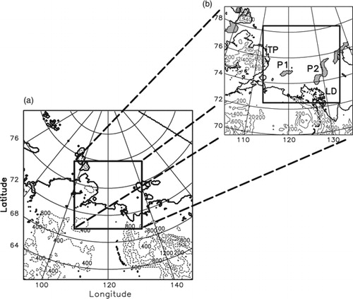
The Laptev Sea is generally covered by pack ice and fast ice from October to June but several flaw polynyas recur at the same positions along the fast ice edge. Zakharov (1966) identified these main flaw polynyas in the Laptev Sea based on their positions (from east to west; see Fig. 1 in Willmes et al. 2011 [this volume]) for locations): the eastern Severnaya Zemlya polynya, the north-eastern Taimyr polynya, the Taimyr polynya, the Anabar–Lena polynya and the western New Siberian polynya. In our study, we apply the sea-ice situation from 29 April 2008, when the western New Siberian polynya (WNS) was well expanded in the eastern Laptev Sea (Fig. 1b). The WNS is the largest polynya in the Laptev Sea and more stable in recurrence than polynyas in the western and north-western Laptev Sea (Bareiss & Görgen 2005).

Fig 1. (a) Consortium for Small-scale Modelling (COSMO) model domain with 15-km resolution (3000 km×3000 km, COSMO-15) and (b) the nesting domain with 5-km mesh size (1000 km×1000 km, COSMO-05). The dashed contour lines represent the topography of the model domain in metres. The polynyas from 29 April 2008 are shown as shaded areas in the 5-km model domain. The rectangle (600 km×600 km) in (b) sketches the area of main interest and indicates the locations of the polynyas we refer to in our studies as P1 (the Anabar–Lena polynya) and P2 (the western New Siberian polynya) as well as the locations of the Taimyr Peninsula (TP) and the Lena Delta (LD).

An energy source like the WNS has a massive impact on the structure of the ABL and the shallow ocean layer (depth around 30 m) in the cold polar climate, especially in winter. With the ocean at freezing point during winter, new ice forms when energy from the ocean is released to the atmosphere in open-water areas. Large quantities of dense brine rejections accumulate at the shelf bottom and contribute to the Arctic deep bottom water after passing the continental slope. These brine inflows originating from the Laptev Sea shelf can have a serious impact on the thermohaline structure and circulation patterns of the Arctic Ocean (Johnson & Polyakov 2001; Dmitrenko et al. 2005). Numbers estimating total ice production in the Laptev Sea are controversial. According to Dethleff et al. (1998)Dethleff et al. (1998a) sea-ice production of 258 km³ within the Laptev Sea flaw polynyas were found for the winter of 1991/92. In contrast, Willmes et al. (2011) estimate a much lower average wintertime ice production—55.2 km³—for the Laptev Sea polynyas, based on remote sensing and data from the National Centers for Environmental Prediction for 1979–2008.

The energy input into the atmosphere changes the structure of the stable ABL dramatically. Developments of mesocyclones have been observed over polynyas (Heinemann 1996; Klein & Heinemann 2001; Hebbinghaus et al. 2007). A couple of numerical simulations have been done in the past using different micro- and mesoscale models to investigate the impact of polynyas and leads on the ABL at high latitudes (Gallée 1997; Dare & Atkinson 2000; Heinemann 2003; Lüpkes, Vihma et al. 2008). Large-eddy simulation models with a very small mesh size of a few metres are necessary for the direct simulation of turbulence above leads and polynyas. While large-eddy simulation models have been successfully applied for studies of small-scale leads (Weinbrecht & Raasch 2001; Esau 2007; Lüpkes, Gryanik et al. 2008), the simulation of polynyas hundreds of kilometres in extent in a realistic environment (with topography and synoptic forcing) can only be done by mesoscale models.

In the next section, the model and the basic settings we employed in our study are described. This is followed by an introduction of the data we used, the design of the simulations and the initial conditions of the six regimes. We then present the results for the impact on the ABL and potential ice production. Finally, we discuss the results and offer our conclusions.

Model description and set-up

In this study we use the mesoscale, non-hydrostatic Consortium for Small-scale Modelling (COSMO) atmosphere model version 4.0 (Steppeler et al. 2003), formerly known as ‘Lokal-Modell’, of the German Meteorological Service. Since 1999, COSMO has been the operational model for weather prediction over Central Europe, with a horizontal resolution of 7 km for Europe and 2.8 km for Germany. The model works on a rotated, spherical coordinate system on a staggered Arakawa C/Lorenz grid. We have chosen 42 layers with 10 layers below 500 m, the lowest layer at 10 m above ground and the top layer at roughly 22 200-m height. Two model domains are applied for nesting purposes with 200×200 grid points each. The coarser one has a horizontal resolution of about 15 km and the finer one of 5 km. For time integration a third-order Runge-Kutta scheme is used. Turbulent processes are parameterized by a prognostic turbulent kinetic energy (TKE) closure with level 2.5. Surface fluxes are parameterized by the TKE-based surface transfer scheme in COSMO. This scheme calculates the transfer coefficients for the exchange of momentum, sensible and latent heat as well as the near surface variables (2 m and 10 m). The zone between the surface and the first model layer is divided in three layers: the laminar boundary layer, the turbulent population layer and the turbulent Prandtl layer. In each of these layers the drag transfer coefficient is calculated separately (Doms et al. 2007). Radiation processes are computed every hour using the parameterization scheme presented by Ritter & Geleyn (1992) and sub-grid moist convection is parameterized using Tietdke's (1989) scheme. The soil temperature and humidity are calculated in the soil module TERRA-ML (Heise et al. 2006), which consists of eight layers beneath the surface; five of these layers are within the upper half metre of the soil column. Initial surface and soil data are taken from the Global Model Extended system of the German Meteorological Service.

The COSMO model has been previously applied in Arctic regions. Klein et al. (2001) simulated the katabatic wind in the transition region between the ice sheet and the tundra over Greenland. Hebbinghaus & Heinemann (2006) analysed snow drift characteristics on the Greenland Ice Sheet. A polar cold air outbreak over Fram Strait was studied by Wacker et al. (2005). Former studies assumed sea-ice surface temperatures to be constant during the simulations (there is no sea-ice module in an operational version so far). This assumption is a strong idealization of sea-ice conditions and does not allow sea-ice response to varying atmospheric conditions.

To study the effect of the Laptev Sea polynya on the ABL, a more realistic description of the sea-ice surface temperature is needed. A thermodynamic sea-ice model was implemented by Schröder et al. (2011 [this volume]). The initial sea-ice coverage, surface temperature and ice thickness field have to be prescribed for each simulation. There is no partial sea-ice cover: the sea-ice fraction is either 0% (open water) or 100% (sea ice). The ice model calculates surface temperatures and ice growth/melting based on the energy budget of the ice layer. No sea ice is produced on grid cells without initial sea ice.

Data and design of the simulations

The model studies were carried out with artificial atmospheric conditions in the Laptev Sea region, while realistic properties of the land surface and the soil layers from the Global Model Extended system and external data were applied.

At first, initial data were prepared (Fig. 2) for the larger model domain with 15-km mesh size (COSMO-15). Mid-winter conditions from 30 December 2007 were used for the surface and soil conditions (Table 1). Sea-ice surface temperature (243 K/253 K), thickness (2 m) and coverage (100%) were set uniformly for the entire Laptev Sea in each COSMO-15 simulation. The initial and boundary atmosphere data for the COSMO-15 runs are defined as horizontally homogeneous. We start with a neutral temperature profile for the lowest 8000 m. During the first 48 h of the simulations, a stably stratified ABL developed, while the surface temperatures decreased because of radiative cooling. Initial temperature profiles with a strong stable stratification were not applied, because they led to an unrealistically strong low level jet above the sea ice due to the model physics and the predefined inversion. The ground surface temperature for the profile calculation was set to the sea-ice surface temperature: 243 K for the cold cases and 253 K for the warm cases. For the upper atmosphere (>8000 m) we assumed an isothermal temperature profile. The initial relative humidity was set to 0%. We assumed a vertically constant initial easterly wind of 3 ms⁻¹, 4 ms⁻¹ and 15 ms⁻¹ (Table 2). We chose these values because the impact of initial wind speed on the resulting wind speed was non-linear. Initial wind speed between 5 and 15 ms⁻¹ from the east led to very similar regimes with an easterly wind speed of 7 to 8 ms⁻¹ for the reference area indicated in (Fig. 3f). Further wind directions were not considered because the WNS polynya (shown as P2 in Fig. 1 only opens by easterly to south-easterly offshore wind directions (perpendicular to the fast ice edge in the eastern Laptev Sea).

Fig 2. The schematic shows the design used in our study. The Consortium for Small-scale Modelling (COSMO) module ‘src_artifdata.f90’ provides the idealized atmospheric conditions. Regimes are shown in Fig. 3 and Table 2.

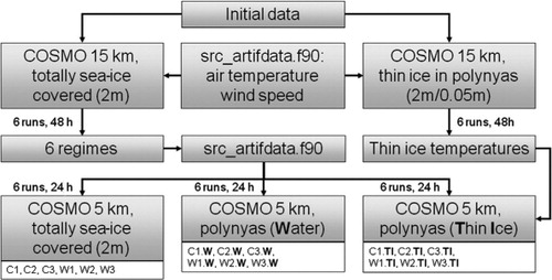
Fig 3. Initial conditions for COSMO-05 obtained from six different COSMO-15 simulations: (a) C1, (b) W1, (c) C2, (d) W2, (e) C3 and (f) W3. Cold regimes are illustrated in (a), (c) and (e) and warm regimes in (b), (d) and (f). The surface temperature is represented by the dashed contour lines with 1-K intervals. Contour minimum for the cold cases is −39°C and for the warm cases −32°C. Vectors indicate 10-m wind velocity (ms⁻¹; every eighth component in meridional [v] and zonal [u] directions). Grey shading indicate the polynya locations (see Fig. 1). The small rectangle in (f) is used to obtain the characteristic properties (10-m wind speed and sea-ice surface temperature) for each simulation (see Table 2). The dot in the centre of the small rectangle marks the position of the profiles shown in Fig. 4.

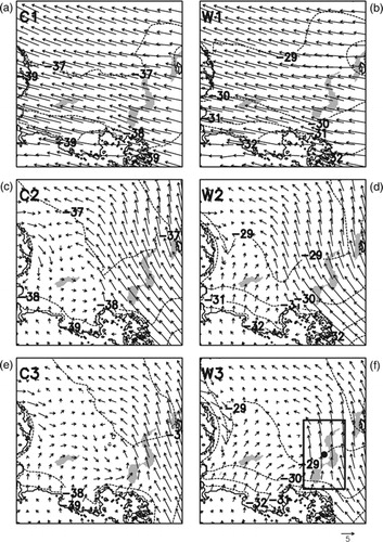
Table 1. Initial, constant and boundary fields for the idealized Consortium for Small-scale Modelling (COSMO) studies.

Parameter	Derived from
Elevation	Global Land One-Kilometre Base Elevation (GLOBE) digital elevation model (1 km; Hastings et al. 1999)
Land cover	GLOBE data set
Soil type	National Aeronautical and Space Administration (5 km; Zobler 1986)
Sea-ice coverage	Advanced Microwave Scanning Radiometer–Earth Observing System (6.25 km; Spreen et al. 2007)
Plant cover	Satellite data with 10′ resolution (Kineman & Hastings 1992)
Leaf area index	Plant cover larger than 0 has a leaf area index=1
Root depth	Global Model Extended (GME; 40 km)
Roughness length	Land: GME (40 km); sea ice: z 0=10^−3 m; water: Charnock (1955)
Soil properties	GME (40 km)
Sea-ice properties	Sea-ice surface temperature: −20.2°C/−30.2°C, water: constant at −1.7°C
Atmosphere	Prescribed in artifdata module of COSMO

Table 2. Start conditions of COSMO-15 and COSMO-05 simulations for cold (C1–C3) and warm regimes (W1–W3). Initial wind speed (v) for COSMO-15 runs applied for all models layers and ice surface temperatures (IST) for the whole sea-ice cover. IST and 10-m wind speed (v_10) as area mean averages of COSMO-05 are from the rectangle in Fig. 3f.

Cold regimes					Warm regimes
	COSMO-15		COSMO-05		COSMO-05		COSMO-15
Regime	IST (°C)	v (ms^−1)	IST (°C)	v_10 (ms^−1)	IST (°C)	v_10 (ms^−1)	IST (°C)	v (ms^−1)	Regime
C1	−30.2	15	−37.3	7.6	−29.7	7.6	−20.2	15	W1
C2	−30.2	4	−37.3	6.8	−29.4	6.3	−20.2	4	W2
C3	−30.2	3	−37.1	4.2	−29.2	4.6	−20.2	3	W3

These COSMO-15 simulations comprised idealized atmospheric conditions, idealized sea-ice specifications and realistic topography with common land use characteristics and were carried out for 48 h. After this period we assumed conditions to be dynamically consistent. The surface roughness over the sea ice, along with the sea-ice thickness and coverage, were kept constant for the simulation period. Therefore, only the sea-ice surface temperature varied. The idealized studies were carried out for winter conditions without shortwave radiation.

Six additional COSMO-15 simulations were performed with a reduced ice thickness of 5 cm within the polynya areas (Fig. 2), retaining the initial surface temperature and roughness length of momentum as for the 2-m ice thickness. The polynya area is taken from Advanced Microwave Scanning Radiometer–Earth Observing System data on sea-ice distribution on 29 April 2008.

Afterwards, we employed the surface and atmospheric characteristics obtained from the last time step (48 h) of the COSMO-15 simulations (without ice thickness reduction in polynya areas) to force six reference runs (100% sea-ice coverage) with 5-km horizontal resolution (COSMO-05). The same boundary file was provided every hour. For impact studies, we changed the surface properties within the polynya area for the COSMO-05 simulations. In the case of open-water polynyas (six runs), the water temperature was set to −1.7°C (freezing point). For thin-ice simulations (six runs), ice thickness is set to 5 cm and thin sea-ice surface temperatures were obtained from the additional COSMO-15 runs with thin ice coverage in the polynyas. The sea-ice fraction threshold to distinguish between sea ice and polynya, necessary for model input due to the restrictions of the sea-ice model, was set to 70%. This commonly used threshold for polynya classification (Massom et al. 1998; Parmiggiani 2006) is suitable for our idealized studies, considering that we want to use different surface properties and varying atmospheric conditions to compare the impact of a polynya system that is constant in extent. The extent of the WNS polynya (P2) in our studies is 7225 km²; the polynya we refer to as P1 has an area of 2375 km².

The resulting cases for the reference runs (without polynya influence) are referred to as C1, C2 and C3 for the cold regimes and W1, W2 and W3 for the warm regimes (Fig. 2), with increasing number indicating decreasing wind speed in the defined rectangle (Fig. 3f). We denote simulations comprising an open-water polynya with the ending W (e.g., C1.W). For thin-ice polynyas the ending TI (e.g., C1.TI) is used.

Start conditions

As explained above, the initial fields for our impact studies were obtained from six COSMO-15 simulations (plus six additional COSMO-15 simulations for cases with thin-ice temperature) with different wind speed and sea-ice temperature initializations. We performed 18 model runs with COSMO-05 to analyse the polynya impact on the ABL concerning three different underlying surface properties at the location of the polynyas for each initial field.

Figure 3 illustrates the six different initial sea-ice and atmospheric conditions of COSMO-05. It is obvious that 48 h is long enough for the large model domain to allow for the development of synoptic and mesoscale systems.

Regimes C1 and W1 are characterized by strong easterly winds in the entire domain with an average speed of 7.6 ms⁻¹ in the eastern Laptev Sea (Table 2). The regimes C2, C3, W2 and W3 are dominated by a heterogeneous wind field above the whole Laptev Sea. While in the eastern region a south-easterly wind direction can be noticed, a weak trough is presented in the western and central Laptev Sea. Lower wind velocities in C2 (6.8 ms⁻¹) and W2 (6.3 ms⁻¹) from the south-eastern region and even lower wind velocities in C3 (4.3 ms⁻¹) and W3 (4.8 ms⁻¹) for the main area of interest are shown.

The weak trough in the western and central part is caused by the extremely cold land mass in the western and southern part of the model domain. The very cold land surface temperatures—up to 20 K colder than the sea-ice surface—act like a barrier for initialized weak winds from the east. The strong south–north temperature gradient causes strong baroclinic conditions along the coast and is responsible for the development of a south-easterly wind direction, with increasing wind speed. The sea-ice surface temperatures between cold and warm regimes differ by around 8 K (Table 2).

Profiles of potential temperature (θ), specific humidity (q), wind velocity (ff) and wind direction (dd) are presented in Fig. 4 from COSMO-05 simulations at initialization time. The θ profiles of case C1 and W3 (Fig. 4a) show a well-developed inversion of up to 1500-m height for C1 and up to 2000 m height for W3. The temperature difference at the first model layer is about 8 K. Specific humidity, which results from evaporation at the surface, reaches maximum values at the lowest model level of about 0.08 g kg⁻¹ for regime C1 and 0.16 g kg⁻¹ for regime W3. The vertical extent of moisture input reaches heights of about 1000 m in regime C1 and 1500 m in regime W3. In both curves there is a noteworthy sharp decrease of air humidity between 150 m and 200 m, where the neutral/slightly stable stratification turns to a strong inversion.

Fig 4. (a) Potential temperature (θ) in °C (solid lines) and specific humidity (q) in g kg⁻¹ (dashed line, upper axis). (b) Wind speed (ff) in ms⁻¹ (solid line) and wind direction (dd) in degrees (dashed line, upper axis). Open circles represent regime C1; closed circles represent regime W3 (Fig. 3, Table 2). Profiles were obtained at the position masked by the dot in Fig. 3f.

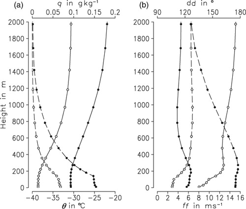
The wind speed and direction are shown in Fig. 4b. Wind speed increases with height from 8 ms⁻¹ at 10 m to 13 ms⁻¹ at 200 m for regime C1, while for regime W3 only a slight increase of about 1 ms⁻¹ occurs. The wind veering with height is simulated with 20° in case C1. In W3 a backing of 50° occurs in the lowest 2000 m.

Impact on the ABL

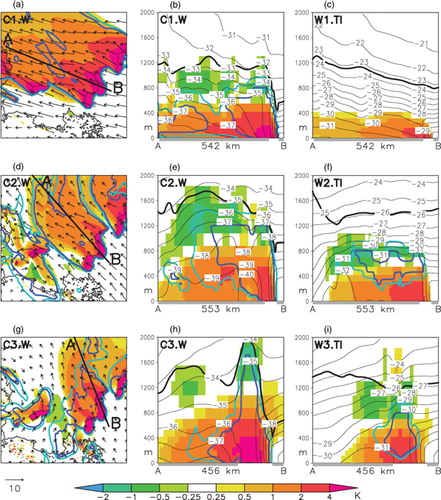
The near-surface atmospheric conditions after a simulation period of 24 h of the COSMO-05 runs are shown in Fig. 5 (cold regimes) and Fig. 6 (warm regimes). In general, an impact of the polynyas on the near-surface wind field and 2-m air temperature is apparent. The influence of polynyas is stronger at cold conditions, which is expected as a result of the higher temperature gradients between the polynya and the atmosphere. The increase of the near-surface temperature downstream of P2 is most extensive in regime C1.W (Fig. 7a). A maximum temperature increase of up to 5 K occurs in the near vicinity downstream of the WNS polynya; even at the eastern coast of the Taimyr Peninsula at a distance of roughly 500 km an increase of 1 K is simulated. In regime W1.TI, the convective boundary layer (CBL) does not exceed 400 m in the vertical (Fig. 7c) due to lower air–sea or air–thin-ice temperature differences and a higher inversion strength compared with the colder regime C1.W (Fig. 7b) with a CBL height of 600-m height. Thus, a shallow CBL is present above the polynya associated with a large-scale, downwind warm plume in case of strong wind speed. Decreasing wind speed enhances the convective heat transfer above polynyas and CBL heights of up to 1200 m develop for the weak wind regime C3.W (Fig. 7h). Compared with the warmer and thin-ice covered case (Fig. 7i), the CBL structure extents to larger heights and the warm anomaly to a larger horizontal scale. Furthermore, a maximum positive temperature anomaly of 5 K in the lowest 400 m is simulated above the polynya.

Fig 5. Atmospheric conditions after 24-h simulation with COSMO-05 for the cold regimes and ice-free polynyas (see initial conditions in Fig. 3). (a), (c), (e) Ten-m wind vectors (every eighth grid point) in ms⁻¹ and 2-m air temperature (2-K intervals between dashed contour lines; minimum contour values −44°C). (b), (d), (f) Anomalies between simulations with polynyas and 100% sea-ice cover after a simulation time of 24 h, with 10-m wind vectors (every fourth grid point) in ms⁻¹. Wind speed anomalies of less than 1 ms⁻¹ are masked out.

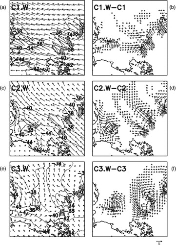
Fig 6. Atmospheric conditions after 24-h simulation with COSMO-05 for the warm regimes and ice-free polynyas (see initial conditions in Fig. 3). (a), (c), (e) Ten-m wind vectors (every eighth grid point) in ms⁻¹ and 2-m air temperature (2-K intervals between dashed contour lines; minimum contour values −40°C). (b), (d), (f) Anomalies between simulations with polynyas and 100% sea-ice cover after a simulation time of 24 h, with 10-m wind vectors (every fourth grid point) in ms⁻¹. Wind speed anomalies of less than 1 ms⁻¹ are masked out.

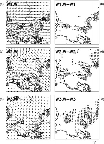
Fig 7. Differences of temperature (shaded) in K between simulations with polynyas and a wholly sea-ice covered Laptev Sea. For location see Fig. 1b. (a), (d), (g) Two-m temperature anomalies in K (shaded) overlaid with horizontal 10-m wind vectors in ms⁻¹ and maximum cloud coverage of the lower 2000 m (light/dark blue contour lines indicate cloud coverage of 10% and 90%). The thick black line sketches the position of the vertical cross-section shown in (b), (e), (h) for cold regimes and in (c), (f), (i) for warm regimes: Temperature anomalies in K (shaded) plotted with potential temperatures (θ) indicated by thin black contour lines with 1-K intervals. The thick black curve marks the 0.01 g kg⁻¹ isoline for specific humidity and the light/dark blue curves mark the cloud coverage isoline of 10%/90%, respectively. The grey line on the x-axis marks the sea-ice cover.

Thermally induced convergence through large horizontal temperature gradients has a visible impact to the near-surface wind field (Figs. 5 and 6). Wind field distortions are stronger for moderate and weak wind conditions than for strong wind regimes and are more spatially limited in warmer regimes. The strong wind regime with 2-m air temperatures of about −30°C shows the weakest modifications of the near-surface wind field (Fig. 6b) compared with weaker wind regimes and colder air temperatures.

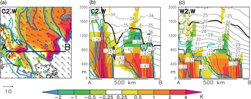
Cyclonic rotation of the near-surface wind is apparent above P1 and in the northern and southern part of P2 for the moderate and weak wind regimes (Fig. 5d, f, 6d, f). Initially calm wind conditions for the cold regimes in the western Laptev Sea and the north-westerly cold air flow of Taimyr Peninsula (Fig. 3c, e) are suitable atmospheric conditions for forcing convection above polynyas. Hence, the most pronounced cyclonic circulations are simulated above P1 for the cold regimes C2.W and C3.W (Fig. 5d, f). Positive temperature anomalies reach up to 1600-m height due to strong convection (Fig. 8b). Also an increase of cloud cover up to 2000-m height occurs for this low-level mesoscale trough, forced by polynya presence in this region. On the other hand, heat advection from the eastern P2 polynya between 300-m and 800-m height can dampen the developing of the cyclonic through (Fig. 8b). Even if the polynya is covered by 5 cm of thin ice, a cyclonic rotation of the wind field is simulated with slightly weaker anomalies (not shown). In the warmer regimes (W2, W3) the development of a pronounced mesoscale trough is retarded due to diminishing temperature gradients at initialization time (Fig. 6, 8c).

Fig 8. Differences of temperature (shaded) in K between simulations with open-water polynyas and a wholly sea-ice covered Laptev Sea. For location see Fig. 1b. (a) Two-m temperature anomalies in K (shaded) overlaid with horizontal 10-m wind vectors in ms⁻¹ and maximum cloud coverage of the lower 2000 m (light/dark blue contour lines indicate cloud coverage of 10% and 90%). The thick black line sketches the position of the vertical cross-section shown in (b) for the cold regime and in (c) for the warm regime: temperature anomalies in K (shaded) plotted with potential temperatures (θ) indicated by thin black contour lines with 1-K intervals (as in Fig. 7). The thick black curve marks the 0.01 g kg⁻¹ isoline for specific humidity and the light/dark blue curves mark the cloud coverage isoline of 10%/90%, respectively. The grey line on the x-axis marks the sea-ice cover.

In general, warm regimes with thin ice coverage within the polynyas show a sharp declining impact on the temperature and wind field anomalies in comparison with colder surroundings and ice-free polynyas. Due to less sensible and latent heat release of a thin-ice covered polynya (Table 3), the CBL can be flattened by 400 m, especially in the weak wind regimes (Fig. 7i). Furthermore, the turbulent heat flux from the ocean into the atmosphere is reduced through a thin ice layer in our studies at strong wind conditions by 274 W m⁻² (44%; Table 3). With less release of latent heat, cloud coverage decreased above polynyas with thin ice coverage (Fig. 7c, f, i). This led to roughly the same surface radiation loss as for an ice-free polynya (Table 4). A maximum value of surface radiation loss is calculated for regime W1.W, caused by less cloud coverage due to a higher dew-point temperature (compared with C1.W) and a fast cloud drift. A relatively high surface radiation loss is simulated for the thin-ice covered polynyas (W1.TI and C1.TI). This is caused by the sharp decrease of cloud coverage in C1.TI (not shown) and the clear sky conditions in W1.TI (Fig. 7c). Hence, polynya induced wind speed, wind direction and air temperature anomalies play a crucial role for cloud processes and, therefore, for the radiation balance above polynyas.

Table 3. Total surface turbulent heat flux (latent [E₀] plus sensible [H₀] heat) and Bowen ratio (β) for polynya P2 (Fig. 1b). Mean area and time averaged values over a simulation time of 24 h.

Regime	Water W m^−2	β=H0/E0	Thin ice W m^−2	β=H0/E0	Δ W m^−2
C1	−619	4.3	−345	8.6	−274
C2	−479	4.6	−308	8.8	−171
C3	−340	4.4	−219	7.3	−121
W1	−470	3.5	−265	5.8	−205
W2	−357	3.8	−223	6.1	−134
W3	−240	3.7	−156	5.5	−84

Table 4. Surface net radiation flux (Q₀) for polynya P2 (Fig. 1b). Mean area and time averaged values over a simulation time of 24 h.

Regime	Water W m^−2	Thin ice W m^−2	Δ W m^−2
C1	−170	−173	+3
C2	−154	−157	+3
C3	−152	−141	−9
W1	−192	−173	−19
W2	−170	−167	−3
W3	−160	−158	−2

The negative air temperature anomaly at the transition between the CBL and the stable stratified atmosphere above is characterized by a maximum cooling of up to 2 K (Figs. 7, 8). Generally, these areas of temperature decline are consistent with the upper boundary of the cloud coverage and the border of the 0.01 g kg⁻¹ specific humidity contour line in the cold regimes (Fig. 7, C1.W–C3.W). Hence, the temperature decline is a result of cooling at the cloud tops (radiation, evaporation). This is confirmed by the clear sky conditions in Fig. 7c and the missing cooling zone above the CBL. The inversion strength will be intensified at the inversion bottom through cloud top cooling processes. Due to higher specific humidity in the warm cases (W1.TI–W3.TI in Fig. 7), the 0.01 g kg⁻¹ border line does not match well with the upper boundary of cooling.

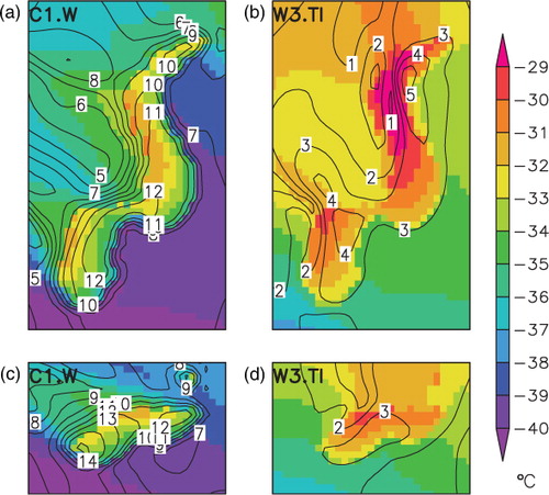
A more detailed view of the 10-m wind speed and 2-m air temperature (Fig. 9) shows strong gradients in the vicinity of the polynyas. Distinct changes of near-surface conditions are obvious at the ice edge of the polynyas in the cold and strong wind regime C1.W (Fig. 9a). Roughly the same temperature amplitude is simulated in the warm and weak wind regime W3.TI (Fig. 9b), while the wind field shows much smoother gradients, apart from the northern area of P2. Marked changes of temperature and wind conditions are caused by polynyas and lead to small-scale variations of ice-production rates that will be discussed below.

Fig 9. Two-m air temperature in °C and 10-m wind speed (contours have 1 ms⁻¹ intervals) as obtained after a simulation time of 24 h for (a) and (b) polynya P2 and (c) and (d) polynya P1. Regime C1.W, with an ice-free polynya, is represented in (a), while regime W3.TI, with 5-cm thin ice is shown in (b). For location see Fig. 1b. The areal extent of (a) and (b) is 150 km×250 km and of (c) and (d) is 150 km×100 km.

Potential ice production

To estimate the amount of newly formed ice in polynyas, potential sea-ice production rates are calculated with following assumptions. The calculation is based on the surface energy balance, assuming that the total atmospheric heat flux (Q_A) is compensated by latent heat release of freezing of sea ice. The Q_A is the sum of the latent (E₀) and sensible (H₀) heat flux and the radiation balance (Q₀). The ice-production rate is then calculated as: (1)

where h is the ice thickness, L the latent heat of fusion (334 kJ kg⁻¹) and ρ the ice density (910 kg m⁻³). It is assumed that newly formed ice does not accumulate in the polynya area. In case of thin ice coverage within the polynya, ice thickness is kept constant during the simulation. Fig. 10 shows the results of simulations of potential sea-ice production rates for the two Laptev Sea polynyas (P1 and P2) without thin ice after a simulation period of 24 h. Additionally, the production rates are given for the entire area of each polynya as the temporal mean over the whole simulation period. The highest rates are derived for the cold and strong wind regime with open-water polynyas (C1.W). The highest value of sea-ice production of more than 24 cm d⁻¹ occurs at the south-eastern part of P2 and the western part of P1. It is striking that there is a strong horizontal gradient of sea-ice production within P2. Differences of about 6 cm d⁻¹ occur between the western and eastern ice edge. An absolute amount of about 1.64 km³ newly formed sea ice is produced within 24 h. This is about 2.5 times higher than the lowest ice-production rate that occurred under the warm and weak wind regime with 5-cm thin ice coverage (Fig. 11f).

Fig 10. Potential sea-ice production rates in cm d⁻¹ (shaded) of the polynya areas P1 and P2 (see Fig. 1b) after a simulation time of 24 h and 10-m wind vectors (ms⁻¹). (a), (b), (c) Potential ice production with open-water polynyas and cold regimes (C1.W, C2.W, C3.W). (d), (e), (f) Potential ice production with open-water polynyas and warm regimes (W1.W, W2.W, W3.W). Potential sea-ice production rates (h) in cm d⁻¹ and sea-ice volume production (V) in km³ d⁻¹ are calculated as an area and time average over 24 h for the polynyas (left value=P1, right value=P2).

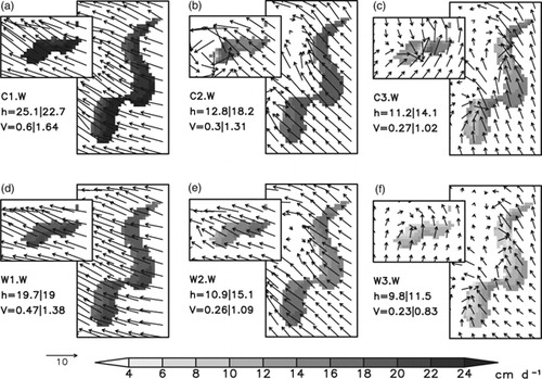
Fig 11. Potential sea-ice production rates in cm d⁻¹ (shaded) of the polynya areas P1 and P2 (see Fig. 1b) after a simulation time of 24 h and 10-m wind vectors (ms⁻¹). (a), (b), (c) Potential ice production with thin ice covered polynyas and cold regimes (C1.TI, C2.TI, C3.TI). (d), (e), (f) Potential ice production with thin ice covered polynyas and warm regimes (W1.TI, W2.TI, W3.TI). Potential sea-ice production rates (h) in cm d⁻¹ and sea-ice volume production (V) in km³ d⁻¹ are calculated as an area and time average over 24 h for the polynyas (left value=P1, right value=P2).

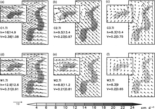
Thermally induced circulations by the polynyas are able to modify the flow for weak wind conditions. The field surface energy fluxes over the polynya areas lead to spatial patterns of ice-production rates. Simulations with strong and moderate wind regimes and 5-cm thin ice coverage show more homogeneous sea-ice production rates in relation to open-water polynyas. The 2-m temperature gradients can differ up to 10 K within a few kilometres between the polynya and the upstream sea-ice cover (Fig. 9).

Variations of wind speed play the dominant role for sea-ice production rates. If we compare the strong wind case (Fig. 10a) with the weak wind case (Fig. 10c) under similar initial temperature (Table 2), ice production decreases from 22.7 to 14.1 cm d⁻¹ for P2. If we compare strong cold conditions (Fig. 10a) with moderate cold conditions (Fig. 10d) under similar initial wind speed, ice production decreases less dramatically from 22.7 to 19 cm d⁻¹. This shows that the high 2-m temperature gradient above the polynya is a secondary atmospheric controlling factor behind wind speed, which leads to further modifications of the existing spatial patterns of ice production (compare Fig. 9a, 10a and Fig. 9b, 11f).

Discussion and conclusions

We studied the impact of a typical flaw polynya system on the ABL in the Laptev Sea through idealized simulations derived from the non-hydrostatic mesoscale COSMO model, with the thermodynamic sea-ice model implemented by Schröder et al. (2011). Six different atmospheric regimes were generated using different initial sea-ice surface temperature and wind speed conditions for a completely sea-ice covered Laptev Sea in a COSMO run with 15-km resolution. In a second run with a higher resolution of 5 km, we investigated the polynya's impact on the ABL in the region.

The studies show an impact on the ABL at distances of hundreds of kilometres away from the polynyas. In the strong easterly wind regime, a positive 2-m air temperature anomaly of 1 K is present over sea ice even further than 500 km downstream of the polynya. In the proximity of polynyas, 2-m air temperature increases up to 5 K. In weaker wind regimes, the horizontal extent of the warming is reduced. Due to weaker wind speed and consequently a more convective ABL, surface heat fluxes lead to a warming of up to 5 K in the lowest 400 m directly above polynyas. Hence, mixed layers develop with depths between 400 m to 1200 m above polynyas and extended warm plumes downwind of the polynyas. Due to cooling at cloud tops, a temperature decline of the inversion bottom layer above the CBL leads to an increase of the inversion strength. For low wind conditions and strong cold temperatures (C2, C3), mesoscale cyclones or mesoscale troughs develop over the western Laptev Sea, which are strongest for runs including ice-free polynyas. This agrees well with simulations made by Hebbinghaus et al. (2007). They found that a vortex over a polynya area being best developed for weak large-scale pressure gradients. In our case, the topography of the Taimyr Peninsula in the vicinity of the small polynya P1 (see Fig. 1b) is an additional forcing factor for mesocyclogenesis by amplifying horizontal and vertical wind shear through cold air flows downward the slopes. The simulations indicate that suitable orography structures can support mesocyclogenesis even in regions with relatively flat orography, compared to Greenland and the Antarctic (Heinemann 1997; Klein & Heinemann 2001; Heinemann & Klein 2003). However, a verification of the mesocyclogenesis is not possible since no in situ measurements are available for the Laptev Sea area. The simulated mixing heights of our study agree well with results presented by Dare & Atkinson (2000).

Cloud coverage above polynyas is caused by surface latent heat release and varies between different simulations. Cloud coverage is greater above ice-free polynyas due to the forced latent heat release from the water surface. Therefore, cloud coverage reduces the differences in the surface radiation loss of ice-free and thin-ice covered polynyas. We have found that thin ice coverage of polynyas can reduce the release of surface turbulent heat flux up to 274 W m⁻² (44%) with cold and strong wind conditions. The decline for warm and weak wind regimes due to thin ice coverage amounts to 84 W m⁻² (35%).

In the proximity of polynyas, large gradients of the 2-m air temperature of up to 10 K occur within a few kilometres. The wind field is also strongly modified by the polynya presence due to thermally induced convergence or even by the development of mesoscale troughs. The polynya-induced small-scale changes strongly modify near-surface conditions (wind field, air temperature) and, therefore, ice-production rates. We derive time- and area-averaged potential ice-production rates between 8 cm d⁻¹ and 25 cm d⁻¹ from our simulations under idealized conditions. Previous calculations of sea-ice production in the Laptev Sea (e.g., Dethleff et al. 1998; Willmes et al. 2011) suffer from missing small-scale atmospheric variability due to the application of global reanalyses model data, in which polynyas are not present. Hence, the use of the temperature and wind field for (long-term) sea-ice production estimation relies on atmospheric conditions that are representative above sea ice. Our results show that this can cause a systematic underestimation of air temperature of up to 10 K and an underestimation of wind speed of up to 5 ms⁻¹. Fortunately, both errors have an opposite effect on sea-ice production. Lower temperatures overestimate ice production, whereas weaker winds underestimate ice production.

Using remote sensing data, Willmes et al. (2011) determined that polynyas are mostly covered with thin ice. Our maximum ice-production rate for ice-free polynyas is about 25 cm d⁻¹; with thin ice coverage, the maximum production rate declines to 16 cm d⁻¹. This matches well with the maximum values of Willmes et al. (2011) . Improving small-scale modelling results will require more investigation of the sea-ice assumptions within a polynya—whether the polynya is ice-free or covered in thin ice and what the thickness of the ice is.

Keeping in mind that the large variability of our ice-production rates results from relatively small variations in forcing fields and boundary conditions, we have demonstrated that the feedback of polynyas and the ABL on a small-scale has a considerable impact on the potential sea-ice production. This uncertainty should be considered in estimations of sea-ice production in polynyas derived from remote sensing data, global circulation models or reanalyses data.

Acknowledgements

This study was funded within the framework of the Laptev Sea System project, supported by the German Federal Ministry of Education and Research (grant no. 03G0639A). The COSMO model was made available by the German Weather Service. Thanks are given to two anonymous reviewers for their helpful comments on the manuscript.

References

- Barber D.G. & Massom R.A. 2007. The role of sea ice in Arctic and Antarctic polynyas. In W.O. Smith Jr. & D.G. Barber (eds.): Polynyas: windows to the world. Pp. 1–43. Amsterdam: Elsevier.
- Bareiss J. & Görgen K. 2005. Spatial and temporal variability of sea ice in the Laptev Sea: analyses and review of satellite passive-microwave data and model results, 1979 to 2002. Global and Planetary Change 48, 28–54.
- Charnock H. 1955. Wind stress over a water surface. The Quarterly Journal of the Royal Meteorological Society 81, 639–640.
- Dare R.A. & Atkinson B.W. 2000. Atmospheric response to spatial variations in concentration and size of polynyas in the southern ocean sea-ice zone. Boundary-Layer Meteorology 94, 65–88.
- Dethleff D., Loewe P. & Kleine E. 1998. The Laptev Sea flaw lead-detailed investigation on ice formation and export during 1991/1992 winter season. Cold Regions Science and Technology 27, 225–243.
- Dmitrenko I.A., Tyshko K.N., Kirillov S.A., Eicken H., Hole-mann J.A. & Kassens H. 2005. Impact of flaw polynyas on the hydrography of the Laptev Sea. Global and Planetary Change 48, 9–27.
- Doms G., Fostner J., Heise E., Herzog H.-J., Raschendorfer M., Reinhardt T., Ritter B., Schrodin R., Schulz J.-P. & Vogel G. 2007. Description of the nonhydrostatic regional model LM. Part II: physical parameterization. Offenbachom Main, Germany: Deutscher Wetterdienst.
- Esau I.N. 2007. Amplification of turbulent exchange over wide Arctic leads: large-eddy simulation study. Journal of Geophy-sical Research-Atmospheres 112, D08109, doi: 10.1029/2006JD007225.
- Gallee H. 1997. Air-sea interactions over Terra Nova Bay during winter: simulation with a coupled atmosphere-polynya model. Journal of Geophysical Research-Atmospheres 102, 13835–13849.
- Hastings D. A., Dunbar P.K., Elphingstone G.M., Bootzan M., Murakami H., Maruyama H., Masaharu H., Holland P., Payne J., Bryant N.A., Logan T.L., Muller J.-P., Schreier G. & MacDonald J.S. (eds.) 1999. The Global Land One-Kilometre Base Elevation (GLOBE) digital elevation model. Version 1.0. Boulder, CO: National Geophysical Data Centre, National Oceanic and Atmospheric Administration.
- Hebbinghaus H. & Heinemann G. 2006. LM simulations of the Greenland boundary layer, comparison with local measurements and SNOWPACK simulations of drifting snow. Cold Regions Science and Technology 46, 36–51.
- Hebbinghaus H., Schlfinzen H. & Dierer S. 2007. Sensitivity studies on vortex development over a polynya. Theoretical and Applied Climatology 88, 1–16.
- Heinemann G. 1996. On the development of wintertime mesoscale cyclones near the sea ice front in the Arctic and Antarctic. The Global Atmosphere and Ocean System 4, 89–123.
- Heinemann G. 1997. Idealized simulations of the Antarctic katabatic wind system with a three-dimensional mesoscale model. Journal of Geophysical Research-Atmospheres 102, 13825–13834.
- Heinemann G. 2003. Forcing and feedback mechanisms between the katabatic wind and sea ice in the coastal areas of polar ice sheets. The Global Atmosphere and Ocean System 9, 169–201.
- Heinemann G. & Klein T. 2003. Simulations of topographically forced mesocyclones in the Weddell Sea and the Ross Sea region of Antarctica. Monthly Weather Review 131, 302–316.
- Heise E., Ritter B. & Schrodin R. 2006. Operational implementa-tion of the multilayer soil model. COSMO Technical Reports No. 9. Offenbach am Main, Germany: Consortium for Small-Scale Modelling.
- Johnson M.A. & Polyakov I.V. 2001. The Laptev Sea as a source for recent Arctic Ocean salinity changes. Geophysical Research Letters 28, 2017–2020.
- Kineman J. & Hastings D. 1992. Monthly generalized global vegetation index from NESDIS NOAA-9 weekly GVI data (Apr 1985-Dec 1988). Boulder, CO: National Geophysical Data Centre, National Oceanic and Atmospheric Administration.
- Klein T. & Heinemann G. 2001. On the forcing mechanisms of mesocyclones in the eastern Weddell Sea region, Antarctica: process studies using a mesoscale numerical model. Meteor-ologische Zeitschrift 10, 113–122.
- Klein T., Heinemann G. & Gross P. 2001. Simulation of the katabatic flow near the Greenland ice margin using a high-resolution non-hydrostatic model. Meteorologische Zeits-chrift 10, 331–339.
- Lupkes C., Gryanik V.M., Witha B., Gryschka M., Raasch S. & Gollnik T. 2008. Modelling convection over Arctic leads with LES and a non-eddy-resolving micro-scale model. Journal of Geophysical Research—Oceans 113, C09028, doi: 10.1029/2007JC004099.
- Lupkes C., Vihma T., Birnbaum G. & Wacker U. 2008. Influence of leads in sea ice on the temperature of the atmospheric boundary layer during polar night. Geophysical Research Letters 35, L03805, doi: 10.1029/2007GL032461.
- Massom R.A, Harris P.T., Michael K. & Potter M.J. 1998. The distribution and formative processes of latent heat polynyas in East Antarctica. Annals of Glaciology 27, 420–426.
- Parmiggiani E 2006. Fluctuations of Terra Nova Bay polynya as observed by active (ASAR) and passive (AMSR-E) microwave radiometers. International Journal of Remote Sen-sing 27, 2459–2469.
- Pease C.H. 1987. The size of wind-driven coastal polynyas. Journal of Geophysical Research—Oceans 92, 7049–7059.
- Ritter B. & Geleyn J.F. 1992. A comprehensive radiation scheme for numerical weather prediction models with potential applications in climate simulations. Monthly Weather Review 120, 303–325.
- Schröder D., Heinemann G. & Willmes S. 2011. The impact of a thermodynamic sea-ice module in the COSMO numerical weather prediction model on simulations for the Laptev Sea, Siberian Arctic. Polar Research 30, article no. 6334, doi: 10.3402/polar.v30i0.6334 (this volume).
- Spreen G., Kaleschke L. & Heygster G. 2007. Sea ice remote sensing using AMSR—E 89 GHz channels. Journal of Geo-physical Research—Oceans 113, CO2503, doi: 10.1029/2005JC003384.
- Steppeler J., Doms G., Schättler U., Bitzer H.W., Gassmann A., Damrath U. & Gregoric G. 2003. Meso-gamma scale fore-casts using the non-hydrostatic model LM. Meteorology and Atmospheric Physics 82, 75–96.
- Tietdke M. 1989. A comprehensive mass flux scheme for cumulus parameterization in large-scale models. Monthly Weather Review 117, 1779–1800.
- Wacker U., Jayaraman Potty K.V., Liipkes C., Hartmann J. & Raschendorfer M. 2005. A case study on a polar cold air outbreak over Fram Strait using a mesoscale weather prediction model. Boundary-Layer Meteorology 117, 301–336.
- Weinbrecht S. & Raasch S. 2001. High-resolution simulations of the turbulent flow in the vicinity of an Arctic lead. Journal of Geophysical Research—Oceans 106, 27035–27046.
- Willmes S., Adams S., Schroder D. & Heinemann G. 2011. Spatio-temporal variability of polynya dynamics and ice production in the Laptev Sea between the winters of 1979/80 and 2007/08. Polar Research 30, article no. 5971, doi: 10.3402/polar.v30i0.5971 (this volume).
- Zakharov V.F. 1966. The role of flaw leads off the edge of fast ice in the hydrological and ice regime of the Laptev Sea. Oceanology 6, 815–821.
- Zobler L. 1986. A world soil file for global climate modelling. NASA Technical Memorandum 87802. Washington, DC: National Aeronautical and Space Administration.