The barrier layer of the Atlantic warmpool: formation mechanism and influence on the mean climate

ABSTRACT

Many coupled general circulation models (CGCMs) tend to overestimate the salinity in the Atlantic warm pool or the Northwestern Tropical Atlantic (NWTA) and underestimate the surface salinity in the subtropical salinity maxima region. Most of these models also suffer from a sea-surface temperature (SST) bias in the NWTA region, leading to suggestions that the upper ocean salinity stratification may need to be improved in order to improve the barrier layer (BL) simulations and thus the SST through BL-SST-intertropical convergence zone feedbacks. In the present study, we use a CGCM to perform a set of idealised numerical experiments to test and understand the sensitivity of the BL and consequently SST in the NWTA region to freshwater flux and hence the upper ocean salinity stratification. We find that the BL of the NWTA is sensitive to upper ocean salinity changes in the Amazon river discharge region and the subtropical salinity maxima region. The BL phenomenon is further manifested by the formation of winter temperature inversions in our model simulations, the maximum magnitude of inversions being about 0.2°C. The atmospheric response causes a statistically significant reduction of mean precipitation and SST in the equatorial Atlantic region and helps improve the respective biases by 10–15%. In the region of improved BL simulation, the SST change is positive and in the right direction of bias correction, albeit weak.

• barrier layer
• upper ocean salinity
• temperature inversions
• Atlantic climate
• Amazon river discharge

1. Introduction

Most coupled general circulation models (CGCMs) fail to accurately simulate the tropical Atlantic climate. A notable feature of CGCM simulations is the bias in sea-surface temperature (SST), with a warm bias over the Southeast Tropical Atlantic (SETA) and a cold bias over the Northwestern Tropical Atlantic (NWTA). The tropical Atlantic SST is an important factor in determining the regional climate of the Atlantic sector and is affected by phenomena, such as El Niño and Southern Oscillation (ENSO), NAO, etc., through atmospheric and oceanic teleconnections (Xie and Philander, 1994; Chang et al., 1997; Saravanan and Chang, 2000; Chang et al., 2006). It also plays a prominent role in the tropical Atlantic hurricane activity (Emanuel, 2005). This underscores the need to understand the sources of these biases in the coupled model simulations.

Carton and Zhou (1997) studied the seasonal cycle of the tropical Atlantic and they attribute the SST cycle in the SETA to the combined effect of coastal upwelling and the changes in latent and sensible heat fluxes due to variation in the trade winds. DeWitt (2005), using an ocean model forced with observed winds, attributed the SST bias primarily to the bias in the zonal wind stress that causes an error in the thermocline and associated entrainment. The erroneous zonal wind pattern not only causes an error in the slope of the thermocline but also causes weak mixing in the East and strong mixing in the West and thus causes the zonal SST bias. Hazeleger and Haarsma (2002) demonstrated the sensitivity of the SST in SETA to upper ocean mixing and thus the entrainment efficiency using both an ocean model as well as a coupled model. Richter and Xie (2008), after an analysis of an ensemble of CGCMs and their atmospheric components, suggested that the bias in coupled model simulations appears to originate from the atmospheric component, particularly convective parameterisations over the Amazon and the NWTA. The failure to simulate good precipitation over tropical South America may be responsible for the weaker-than-observed zonal winds in the eastern equatorial Atlantic, which in turn does not allow the cold tongue to develop during boreal summer. Huang et al. (2007) attributed the SST bias to the models inability to simulate stratus clouds in the SETA region along with the zonal windstress bias in the equatorial Atlantic region.

The upper ocean interacts with the atmosphere, exchanging heat, momentum and buoyancy fluxes. These fluxes jointly determine the climate of the coupled system. The upper ocean density stratification determines the extent to which the atmospheric forcing can influence the ocean interior through turbulent mixing. Mixing occurs when the turbulent kinetic energy imparted by wind mixing or convective instability caused by surface cooling or evaporation is sufficiently strong to overcome the potential energy barrier imposed by density stratification. Mixing affects the SST by regulating the mixed layer heat (MLH) budget through entrainment of subsurface water into the mixed layer and in this way exerts a certain degree of control on the climate of the coupled system.

The tropics are regions of strong air–sea coupling and thus it is very important to understand the role played by the various factors that determine the upper ocean density structure. Salinity is an important variable of the ocean, which plays a pivotal role along with temperature in determining the density and hence the stratification of the ocean. Traditionally, the importance of salinity has always been recognised in the high-latitude deep-water formation regions of the world, in the context of the thermohaline circulation, but not so much so in the tropics.

The importance of the role played by salinity in the tropics was first recognised by Miller (1976), who extended the thermally mixed upper ocean layer theory originally developed by Kraus and Turner (1967) and later by Denman (1973) to include the effects of salinity and found that it has a significant influence on the heating characteristics of the upper ocean mixed layer and is essential for the formation of temperature inversions. But the real interest in salinity began with the focus on the ENSO gaining momentum, when it was recognised that the upper ocean salinity in the Western Pacific warm pool region might have a role to play in the onset of El Niño. This eventually led to the discovery of the salt-stratified barrier layer (BL) (Godfrey and Lindstrom, 1989; Lukas and Lindstrom, 1991). Recent studies also confirm the importance of upper ocean salinity in the Western Pacific. Maes et al. (2006), using data obtained from TAO/TRITON moorings, demonstrated the significance of upper ocean salinity in the Western Pacific warm pool in controlling air–sea interactions. They show that the BL at the eastern edge of the warm pool is very well correlated with the 28 C isotherm near the dateline. Using a regional ocean–atmosphere coupled model, Maes et al. (2002) illustrated the importance of salinity of BLs for the heat build-up in the pacific warm pool, which possibly triggers the ENSO.

The BL mechanism is perhaps one of the most important mechanisms through which salinity directly plays a role in air–sea coupling. The BL occurs when the mixed layer depth (MLD), which is homogenous in density, is shallower than the isothermal layer depth (ILD), which is homogenous in temperature. In this situation, the distance separating the top of the pycnocline from the top of the thermocline is known as BL, as it acts like a barrier to vertical mixing. Even though it occurs in many oceanic regions, its significance is amplified in the tropics due to the effect of strong air–sea coupling in the region. In the tropics, the three important regions of BL formation are the Western Pacific warm pool, NWTA and the Bay of Bengal in the Indian Ocean. Sprintall and Tomczak (1992), based on observational data, pointed out that the formation mechanisms of the BLs are different from one tropical ocean to another.

From the tropical Atlantic annual Evaporation–Precipitation (E–P) balance analysis, it becomes clear that the NWTA or the region to the East of the Caribbean Sea is a place of net loss of freshwater (Dorman and Bourke, 1981; Schmitt et al., 1989). Thus the freshwater in the surface has to be obtained from other sources like local rivers. One of the dominant factors in the freshwater balance in this region is the combined discharge of the mighty Amazon and Orinoco river systems, which when put together form the biggest river system in the world in terms of discharge (0.2 Sv). As a result, thick BLs are formed off the river mouths (Pailler et al., 1999). The Guyana current takes a significant portion of this water into the Caribbean Sea during boreal summer and fall (Hu et al., 1997). Foltz and McPhaden (2008) also showed that the Amazon outflow is advected northwestward towards the Caribbean and conclude that this advection is the main term in the surface salinity balance of that region. Subsurface warm and high-salinity waters are formed in the subtropical gyres of the respective hemispheres and are subducted as salinity maximum water (SMW). The surface of freshwater along with the subsurface of SMW presumably form the thick BLs observed here during boreal winter (Sprintall and Tomczak, 1992). The region to the North of South America and East of the Caribbean basin has thick persistent BLs and, according to Mignot et al. (2007), is one of the most prominent structures of the global tropics and subtropics. These BLs, when they form during late fall and early winter, weaken entrainment and do not allow atmospheric cooling to penetrate into deeper waters. Thus, this region is usually associated with a temperature inversion during the winter (Breugem et al., 2008).

It was shown that the barrier layer thickness (BLT) indeed has an impact on SST in the tropical Atlantic (Foltz and McPhaden, 2009). As the BL plays a role in trapping the heat within the upper ocean layer, it may also affect the Atlantic hurricane activity (Ffield, 2007; Vizy and Cook, 2009). The Amazon plume, which extends into the Caribbean Sea, has relatively high SSTs. The high SSTs are sustained for great distances in the plume due to the BL effect, which may significantly impact the air–sea coupling processes of hurricanes passing these regions by alleviating the SST cooling due to the more stable stratification of the BLs. Hence, such BL effects on the tropical climate and hurricane simulations in CGCMs may not be negligible. For long-term trend prediction in Atlantic hurricanes, we need realistic BL simulations in CGCMs.

Many CGCMs underestimate the freshening due to river discharge in this region and also have a bias in precipitation due to an error in the mean position of the intertropical convergence zone (ITCZ) (Breugem et al., 2008). These two factors together contribute to the upper ocean salinity bias. This can potentially cause a bias in the density stratification and hence the BL formation. Breugem et al. (2008) suggested that upper ocean salinity stratification needs to be improved in the model to allow a realistic representation of BL dynamics and associated feedbacks among BL, SST and ITCZ.

Most studies in the past have focused on the effects of heat and momentum flux exchanges between the atmosphere and ocean, fewer studies have focused on feedbacks associated with freshwater changes. Masson and Delecluse (2001) have performed a series of sensitivity experiments with varying river discharge to observe the effect of Amazon river discharge on the tropical Atlantic climate. However, their experiments were carried out with an ocean general circulation model, thus leaving out the scope for potentially important air–sea interactions to play a role. Here, we have devised a set of idealised sensitivity experiments with a CGCM to examine not only the effect of freshwater flux on the upper ocean salinity stratification but also its effect on the SST in the NWTA region through BL-SST-ITCZ feedbacks.

The organisation of the paper is as follows. Section 2 gives a description of the model, the experiments performed and the data used for analysis. In Section 3, the surface ocean response to the (E–P) forcing is examined in various experiments while the indirect response is discussed in Section 4. Sections 5 and 6 pertain to temperature inversions and the MLH budget analysis, respectively. Finally, a brief summary and discussion is given in Section 7.

2. Model, data and experiments

The model we use for the present study is the fully coupled climate model CCSM 3.0 developed at NCAR. It consists of the Community Atmosphere Model (CAM), the Community Land Model (CLM), the Parallel Ocean Program (POP) and the Community Sea Ice Model (CSIM). These four component models interact with each other through a coupler (CPL). Analysis of its performance at high resolution is given by Collins et al. (2006). We use the model at its standard resolution which has CAM and CLM configured at a resolution of T42 (2.8×2.8  approximately) while POP and CSIM are set at a resolution of gx1v3, which is 1  in longitude and variable in latitudinal direction, with a fine resolution of 0.3 near the equator. POP has 40 vertical levels, increasing monotonically from 10 m near the surface to 250 m at the bottom.

First, we consider the simulated climate of this model. Figure 1 shows the model bias in SST, SSS and precipitation. The model bias in SST and SSS is obtained by subtracting the climatological annual mean SST and SSS (Locarnini et al., 2010; Antonov et al., 2010) from the corresponding model simulated annual mean based on 50 yr of the model run. In the SST (Fig. 1a), the model shows a warm bias in the SETA and a cold bias in the NWTA region. The warm bias has a maximum value of about 5 C while the cold bias has a maximum value of about 3 C. On the other hand, the model shows a positive SSS bias (Fig. 1b) with a peak value of about 1 g kg⁻¹ in the NWTA region. In the south tropical Atlantic, the SSS shows a negative bias with a peak value of about 4 g kg⁻¹. Another negative SSS bias occurs near the northern subtropical salinity maxima region. The precipitation bias, shown in Fig. 1c, is obtained by taking the difference between the model annual mean precipitation in the control run (CR) and the annual mean precipitation from CMAP (Xie and Arkin, 1997). The most glaring error of the precipitation is the positive bias over the SETA region and the negative bias over the Amazon region. This error pattern is indicative of a Southward shift of the ITCZ, which sparks the hypothesis by Breugem et al. (2008) that the erroneous BL simulation in this region may contribute to the bias in SST through the BL-SST-ITCZ feedback mechanism.

Fig. 1.  Mean biases in the model simulation. (a) SST ( C), (b) SSS (g kg⁻¹), (c) precipitation (mm d⁻¹) and (d) BLT (m).

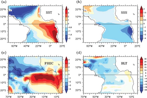
In Fig. 1d, the mean bias of the simulated BLT model is shown. The computation of BLT is done as follows. The ILD is defined as the depth where the potential temperature ( ) decreases by 0.2 C with respect to its value at 10 m. The MLD is the depth where the potential density (σ) has increased by a value that corresponds to a decrease in potential temperature by 0.2 C, with respect to its reference value at a depth of 10m. The BLT is then defined as the ILD minus the MLD (de Boyer Montégut et al., 2007). The observational climatology of BLT and MLD was obtained from ‘Laboratoire d Oceanographie et du Climat (http://www.lodyc.jussieu.fr/cdblod/blt.html)’. As seen from Fig. 1d, the model underestimates the BL in the NWTA region with most underestimation occurring between 60 W–50 W and 10 N–20 N. This bias is not just inherent to CCSM but to most currently existing coupled models. Also, there is a small region in the Caribbean basin between 15 N and 20 N and to the West of 65 W where the BL is overestimated (Breugem et al., 2008).

To study factors that cause these biases, we conduct four ensembles of experiments with the coupled model. First, we perform a 50-yr control simulation with an initial condition obtained from a spin up run. The restart file of the spin up run is obtained from ‘NCAR (www.earthsystemgrid.org)’. We then divide the 50-yr long run into five sets of 10-yr runs and use the first month of each of these five sets as our initial condition and perform simulations with each initial condition. With each of these five initial conditions, we then add a constant precipitation anomaly of +4 mm d⁻¹ in the region of Amazon discharge to the model and integrate the model for 10 yr. The value of 4 mm d⁻¹ is estimated from the precipitation bias over Northern South America. This experiment is referred to as EXP1, where we attempt to emulate the Amazon–Orinoco river discharge and examine the effect of lowering the upper ocean salinity in this region.

In reality, most of the rainfall that feeds the Amazon basin occurs in the South between 0 S–10 S and 70 W–50 W. However, the model is unable to accurately simulate the rainfall in the catchment basin and consequently the Amazon discharge (Dickinson et al., 2006). Misrepresentation of precipitation and soil moisture physics is supposed to be the origin of the bias. The forcing we specify attempts to overcome this model inability. By applying the forcing in the ocean model close to the river mouth and directly over the ocean, we are trying to artificially simulate the effects of the Amazon river discharge and overcome the discrepancies which might arise from specifying the freshwater flux through the atmosphere model and from translation of the freshwater flux into river discharge at the Amazon mouth by the land model.

In the next set of experiments, we add a constant precipitation anomaly of –4 mm d⁻¹ in the subduction region of the northern subtropical salinity maxima, along with the forcing described earlier in EXP1. We refer to this experiment as EXP2. Since primarily subduction processes control the subsurface salinity in the NWTA region, EXP2 allows us to examine the effect of correcting the bias in subsurface salinity on improving the BL simulation in the NWTA region (Sprintall and Tomczak, 1992). Finally, to test the model sensitivity, we double both the forcings in EXP3. A brief description of the experiments is given in Table 1 and the regions of forcing are shown in Fig. 2.

Fig. 2.  Regions and the magnitudes of the forcing applied in model experiments.

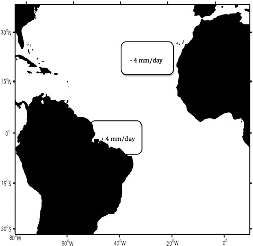
Table 1. Description of various model simulations performed

Experiment	Description
CR	Control run, 50 yr long
EXP1	Five 10-yr runs with freshening in the Amazon region
EXP2	Five 10-yr runs with both, freshening in the Amazon region as well as increased salinity in the subtropical salinity maxima region
EXP3	Five 10-yr runs with double the forcing in EXP2

Using different ocean and atmosphere initial conditions for each simulation allows us to form an ensemble of runs subject to the same salinity forcing. An ensemble average of these runs can reduce the influence of internal variability of the system, so that the response of the coupled system to the salinity forcing can be more clearly delineated. In each of these experiments, after we perform the simulations with each of the five initial conditions, we perform an ensemble average to generate a single time series of 10 yr. We then analyse the ensemble averaged model simulations to identify the factors controlling the extent and magnitude of BLs in the NWTA region.

3. Surface ocean response to the (E–P) forcing

We begin by examining EXP1 in Fig. 3. The changes in mean SST and SSS are shown in Fig. 3a and b, while the mean changes in MLD and BLT are shown in Fig. 3c and d, respectively. The change is obtained by taking the ensemble average of time mean for EXP1 and the CR and subtracting the latter from the former.

Fig. 3.  Mean changes in EXP1 (a) SST ( C), (b) SSS (g kg⁻¹), (c) MLD (m) and (d) BLT (m) (closed contours show those regions where the changes satisfy the Student's t-test for statistical significance at 95% confidence level).

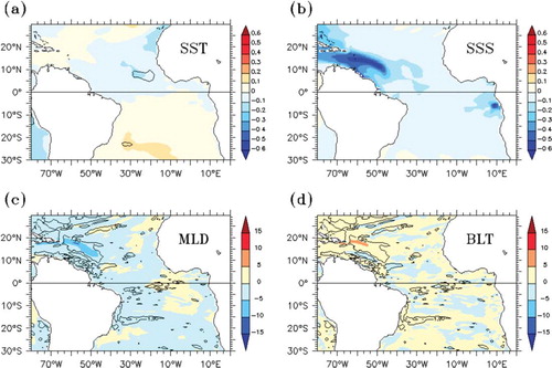
The Amazon river discharges about 0.17 Sv on an average from its mouth located at around 50 W, 0 N. The river discharge varies from about 112 000 m³ s⁻¹ in November to about 229 000 m³ s⁻¹ in May–June. Most of the discharged water is carried Northwestward initially by the Guyana current with a maximum correlation of the downstream river plume SSS with the SSS at Amazon mouth occurring at Barbados with a lag time of 2 months. The water then flows further westward through the islands of Lesser Antilles into the Caribbean Sea. From there, the Caribbean current takes it Northward and westward and the water finally exits through the Yucatan Channel (Hellweger and Gordon, 2002). Consistent with this depiction, we find that most of the freshening is carried Northwestward towards the Caribbean islands with a peak freshening of about 1 g kg⁻¹ due to the strong North Brazil and Guyana current system, which creates a surface divergence near the Amazon mouth and a convergence in the Caribbean Sea. There is some eastward propagation of the surface freshening and this could be attributed to the seasonal NECC.

Let us now consider the SST change in Fig. 3a. A Student's t-test is performed based on the five-member ensemble to check the statistical significance of the SST change and it is found that apart from a few small regions, there are no major regions where the t-value satisfies the criterion for 95% confidence level. Thus the SST change in this experiment is not statistically significant. To the east of the Caribbean Sea, between 50 W and 65 W and at around 18 N, we find an increase of BLT with a maximum increase of about 10 m, as seen in Fig. 4c. Coinciding with this is the reduction in MLD with a maximum reduction of about 10 m (Fig. 4d). The changes in BLT and MLD, which are statistically significant, suggest that the increase in BLT is brought about by the same factor that causes a decrease in MLD, which is surface freshening. This is especially evident when we consider that there is hardly any change in the ILD. A time-series analysis shows that the MLD and BLT are negatively correlated with a correlation coefficient of –0.65 at zero lag. Another interesting finding is that the region of maximum MLD change does not coincide with the region of maximum SSS change, but with the maximum gradient in SSS.

Fig. 4.  The mean changes along 57 W and between 10 N and 25 N for (a) SSS (g kg⁻¹), (b) d(▵SSS)/dy (g kg⁻¹ m⁻¹) and changes in (c) MLD (m).

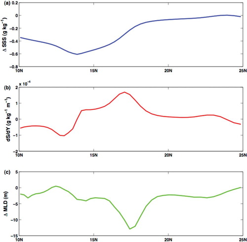
The mean changes in SSS, the meridional gradient in SSS anomaly d▵SSS/dy and MLD, along 57 W and between 10 N and 25 N, are shown in Fig. 4a–c, respectively. The maximum decrease of salinity occurs at around 14 N by about 0.6 g kg⁻¹ while both d▵SSS/dy and MLD change reach their maxima at around 18 N. Increase in the salinity gradient occurs where the freshwater meets saltier water and slides over it, causing the increase in stratification and the reduction in MLD. The same can be seen when we look at the change in static stability (not shown).

In the NWTA, the surface salinity is heavily influenced by the river discharge from Amazon to Orinoco river systems while the subsurface salinity is controlled primarily by the remote mechanism of subduction. Almost 8 Sv of the SMW flows into the Caribbean after sinking from the Northern Hemisphere subtropical region (Blanke et al., 2002). The model fails to accurately simulate the subtropical salinity maxima region. In the Northern Hemisphere, the high SSS is not only lower but also displaced to the West of the actual region. The high SSS water subducts as a shallow subtropical salinity maximum and spreads both southward and westward. This high-salinity water underlying the freshwaters of the Amazon–Orinoco river system is partially responsible for the formation of the shallow pycnocline. To validate our conjecture, we further design a set of ensemble experiments, EXP2, as discussed in what follows.

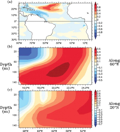
The salinity change induced in EXP2 is shown in Fig. 5. From the SSS change shown in Fig. 5a it can be seen that in addition to the surface freshening from the Amazon mouth to the Caribbean as shown in the previous experiment, we also see high-salinity water flowing southwestwards from the region of subtropical salinity maxima. Figure 5b shows subsurface salinity changes along a North–South transect at 60°W while Fig. 5c shows the same along an East–West transect at 20 N. From these two figures, it is clear that high-salinity anomalies sink with the subtropical salinity maxima waters and flow southward and westward towards the Caribbean, where they lie beneath the low-salinity anomalies propagating from the Amazon discharge region. Together they maintain the shallow pycnocline observed in this region. Every year, beginning in May, the NECC develops as a continuous eastward flow. The NECC weakens considerably by November and due to this, most of the salinity maxima water flows westward during winter. This has been proposed to be a main cause for thick BLs to form during the winter months in the Caribbean (Sprintall and Tomczak, 1992).

Fig. 5.  Illustration of the mean salinity changes (g kg⁻¹) induced in EXP2. The change in surface salinity is shown in (a), the subsurface salinity change along 60 W in (b) and along 20 N in (c).

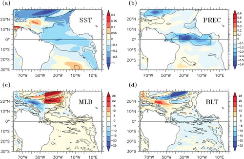
In Fig. 6, we examine the response of the model to the salinity change. The changes in mean SST and precipitation are shown in Fig. 6a and b, respectively. Figure 7c and d shows the changes in mean MLD and BLT, respectively. The first thing to note is that the regions of maximum change in BLT, MLD and SST coincide. The closed contours show those regions where the change is statistically significant at 95% confidence level. The mean change in BLT is over 20 m and the mean MLD change is of the same order. This shows that not only a surface freshening but also a subsurface salinity maximum is required for BL formation in this region. The relative extent to which the model responds to the changes in these two factors would depend on the respective magnitudes of bias. There is a positive SST change in the region of BL increase of about 0.1–0.2 C, but the change does not satisfy the t-test and hence is not statistically significant. However, there is statistically significant SST cooling of about 0.6 C and reduction in precipitation of about 0.2mmd⁻¹ in the region between 60 W and 40 W and between 25 N and 30 N.

Fig. 6.  The results from EXP2 are shown. The mean change in SST ( C) is shown in (a), the mean precipitation change (mm d⁻¹) in (b), the MLD change (m) in (c) and the mean BLT change (m) in (d) (closed contours show those regions where the changes satisfy the Student's t-test for statistical significance at 95% confidence level).

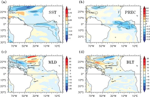
Fig. 7.  Idem as for Fig. 7, but now for EXP3.

To test the sensitivity of the model response to the forcing amplitude, we perform EXP3. The results are shown in Fig. 7. The salinity changes are regionally similar to the salinity changes in EXP2 but the magnitude of maximum salinity change is about 1.5 g kg⁻¹. Again, like in the previous experiment, we find a decrease of MLD and an increase of BLT in the Caribbean with the respective changes being higher than in EXP2 (about 25 m). Similar to EXP2, we have significant negative SST and precipitation anomalies to the North and North-East region of BL increase but with a maximum magnitude of about 1 C and 0.5 mm d⁻¹, respectively.

We note that these cold anomalies do not appear in EXP1. This leads us to the question as to what the source of this cooling could be. There are two important observations that are worth noting. The first is that the cooling occurs only in those experiments where we increase the salinity in the salinity maxima region. The second is that the magnitude of cooling responds almost linearly to forcing magnitude. This suggests that the cooling may be a direct response to the salinity changes in the subduction region. When we look at the evolution of SST (not shown), it is very clear that the cooling pattern resembles the pattern of salinity changes at the surface. Also, when we look at the change in MLD (Figs. 6 and 7), we can see that the regions of MLD increase coincide well with regions of cooling. To increase the salinity, we have added a positive E–P anomaly in this region. More evaporation occurs leading to an increase in surface salinity, which in turn destabilises the water column, resulting in an enhanced mixing. The convection within the oceanic boundary layer in the K profile parameterisation mixing scheme, which is employed in this model, can penetrate into the thermocline and cause an increase in the mixed layer (Large et al., 1994). Therefore, the evaporation forcing is likely to be responsible for the cooling.

4. Indirect response to the forcing

Both in EXP2 and EXP3, there is SST cooling and reduction in precipitation in the equatorial Atlantic region. The maximum SST cooling in EXP2 is about 0.2 C and the maximum reduction in precipitation is about 0.4 mm d⁻¹. Thus, the improvement in equatorial Atlantic SST and precipitation bias is only about 10% of the mean bias. In EXP3, there is statistically significant SST cooling with a maximum magnitude of about 0.2–0.6 C near the equator. The magnitude of precipitation anomalies straddling the equator in this experiment is also higher (about 0.8 mm d⁻¹) and is statistically significant. The improvement in equatorial Atlantic SST and precipitation bias in this experiment is about 15%. To establish the causal relationship between SST and precipitation, Singular Value Decomposition analysis was performed. The region where maximum covariance occurs is between 35 W and 20 W and between 0  and 5 N. Up to 47% of the covariance can be explained by the first three empirical modes. For this region, the time series of SST and precipitation anomalies are correlated at 0.53, suggesting that the SST change causes the precipitation anomaly.

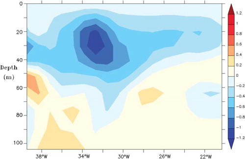
To explain the cooling in the equatorial region, we need to consider changes in atmospheric circulation as shown in Fig. 8. The cooling to the North and Northeast region of BL increase strengthens the Azores high or the North Atlantic Anticyclone and consequently generates easterly wind anomalies near the equator. These zonal wind anomalies cause enhanced equatorial upwelling and SST cooling. This cooling consequently results in enhanced surface wind divergence and a reduction in precipitation. A time series analysis shows that for the region averaged between 34 W and 30 W on the equator, the zonal wind anomalies and SST anomalies are correlated significantly at 0.19 with the zonal wind stress anomalies leading the SST anomalies by a month. Also, for the same region, the anomalies of divergence of surface wind stress are significantly correlated with SST anomalies at zero lag with a correlation coefficient of –0.58. The correlation coefficients obtained satisfy the Student's t-test at 95% confidence level. Figure 9 shows the mean changes in oceanic vertical velocity for EXP3 along the equator. We can clearly see that upwelling is increased, with maximum increase occurring between 34 W and 30 W. Thus we suggest that when the forcing is strong, the response in the atmospheric circulation triggers a significant equatorial response in SST through changes in local upwelling, which in turn causes the response in surface wind divergence and precipitation.

Fig. 8.  The mean changes in circulation of surface winds in EXP3. The units are in N m⁻².

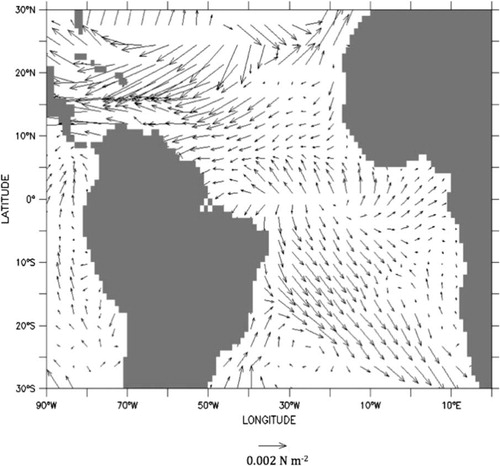
Fig. 9.  Mean changes in vertical velocity along the equator and between 40 W and 20 W. Velocity is positive downwards and each unit is 10⁻⁶ m s⁻¹.

5. Temperature inversions

One of the signatures of BLs in the NWTA is the formation of temperature inversions during boreal winter months. Beginning in late fall, the atmosphere tends to cool the surface ocean. Normally, surface winds would mix up the upper ocean and cause a uniform cooling of the mixed layer or isothermal layer. However, in the presence of a BL, the strong pycnocline below the mixed layer does not allow wind mixing to penetrate below the mixed layer. Consequently, the water below the density mixed layer is not cooled and is able to retain its temperature. As a result of this, temperature inversions begin to form. Typically, entrainment would cause a cooling of the mixed layer but in cases where we have subsurface temperature inversions, entrainment would cause a warming of the mixed layer temperature (Breugem et al., 2008). This process helps in alleviating the effect of atmospheric cooling on SST in the NWTA. The effect of improved BL simulation on the temperature inversions found in this region is now examined.

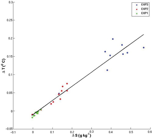
We take the ensemble averages for each experiment and compute the maximum subsurface temperature difference (▵T) across the base of the mixed layer, averaged over the region between 65 W and 50 W and between 18 N and 20 N and for the winter seasons in each of the 10 yr. ▵T=T _–h –T _ml, where T _–h is the temperature below the mixed layer and T _ml is the temperature at the base of mixed layer. Thus a positive ▵T indicates an inversion in subsurface temperature. ▵S is the corresponding salinity difference across the mixed layer. Figure 10 shows the scatter between ▵T and ▵S. In EXP1, the increase in BLT is about 10m and the vertical salinity stratification is not strong enough to support an inversion in temperature. However, in EXP2 the BLT increase is much larger (about 20m) and the salinity gradients induced are substantial enough to induce temperature inversions. The maximum inversion in this experiment is about 0.07 C. The BLT increase in EXP3 is even larger (about 25m) and thus the higher salinity gradients are able to support a stronger temperature inversion of about 0.2 C.

Fig. 10.  Winter vertical subsurface temperature and salinity differences below the mixed layer plotted against each other for the three experiments. Values have been averaged over the region between 65 W and 50 W and between 18 N and 20 N.

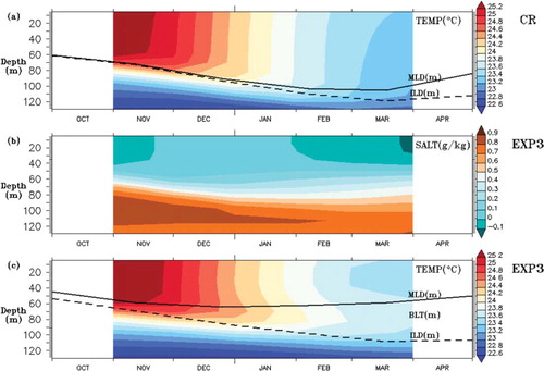
The effect of improved BL simulation on the formation of temperature inversions is shown in Fig. 11. The top panel (Fig. 11a), corresponding to the winter of year 4 from the 10 yr CR, shows that the MLD is almost as deep as the ILD, as a result of which there are no thick BLs. This means that below the MLD, the haline stratification is not strong enough to sustain the formation of an inversion in temperature and thus no inversions develop. The middle panel (Fig. 11b) shows the development of the subsurface salinity anomaly in year 4 of EXP3. The intrusion of a high-salinity tongue, which can be seen centred at around 100 m, is a result of the enhanced subduction as discussed earlier. This increased salinity in the subsurface is responsible for the shoaling of the pycnocline and the formation of thick BLs. From Fig. 11c, it is evident that the thick BLs result as a consequence of the subsurface salinity anomaly, which in turn supports the formation of temperature inversions. It should be noted that the ILD in EXP3 is almost identical to the ILD in the control simulation, suggesting that the inversions are entirely induced by changes in MLD and consequently BLT.

Fig. 11.  The subsurface temperature during the winter of year 4 in the CR is shown in (a). (b) and (c) show the subsurface salinity anomaly and the subsurface temperature, respectively, during the winter of year 4 in EXP3. Values have been averaged over the region between 65 W and 50 W and between 18 N and 20 N.

6. Heat budget analysis

To better understand the SST change in the region of BL increase, we consider a simplified MLH budget equation (Moisan and Niiler, 1998), which can be written as:1

The aforementioned simplified MLH equation was also used by Foltz and McPhaden (2009) in the analysis of BL in the central tropical North Atlantic. The term on the left-hand side, ?C _p h , represents the rate of change of MLH storage. Here ? is the mixed-layer averaged density, C _p is the specific heat of sea water (4000 J kg⁻¹ K⁻¹), h is the depth of the mixed layer and T is the mixed-layer averaged temperature. The first term on the right hand side, q ₀, represents the net surface heat flux (SHF) corrected for the penetration of short wave radiation at the base of the mixed layer. The second, ?C _p h (v. T), represents the advective heat flux (AHF) where v is the mixed-layer averaged velocity. The third term, q _–h , represents the heat flux due to entrainment and other turbulent processes at the base of the mixed layer (turbulent heat flux, THF), which is obtained as a residue. ɛ is the error.

The short wave radiation penetrating the base of the MLD can be estimated as:2

Here, the parameters A ₁, A ₂, B ₁ and B ₂ are chlorophyll-based parameters, q _sfc is the short wave radiation incident at the surface, the albedo ‘a’ is assumed as 6% (Foltz and McPhaden, 2009) and h is the MLD. The climatology of chlorophyll distributions is based on Sea-viewing Wide Field-of-view Sensor (SeaWIFS) data and the chlorophyll-based parameters A ₁, A ₂, B ₁ and B ₂ are obtained from Ohlmann (2003). The SeaWIFS chlorophyll climatology was obtained from NCAR (Nancy J. Norton, personal communication, 2009).

Figure 12 shows the evolution of the anomalies for each of the terms in the MLH budget in EXP1, EXP2 and EXP3 for the region averaged between 65 W and 50 W and between 18 N and 20 N. All terms are smoothed with a 5-month running mean and the corresponding error bars are indicated. Figure 12a shows the MLH anomalies, Fig. 12b shows the SHF anomalies, Fig. 12c shows the AHF anomalies while 12d shows the THF anomalies. We caution that THF is calculated as a residue and thus may not be an accurate representation of entrainment and other turbulent processes at the base of the mixed layer.

Fig. 12.  Time evolution of the MLH budget terms (W m⁻²) with error bars indicated. The evolution of MLH in (a), SHF in (b), AHF in (c) and THF in (d) for the various cases as depicted in the legend. All time series are at a running mean of 5 months. The first and last years have been removed due to box-car smoothing. All values have been averaged over the region between 65 W and 50 W and between 18 N and 20 N.

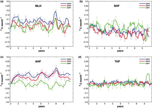
In evaluating different components of the heat budget, we note that in MLH, AHF and SHF the long-term changes are comparable to the seasonal variations, whereas in THF the former are much weaker than the latter. Mean changes in MLH are 0.03 and 0.08 °C month⁻¹, respectively, in EXP2 and EXP3 implying a slight increase in the MLH storage in the region of BL increase. The changes in mean SHF are estimated to be about − 0.03 and −0.05  C month⁻¹ in EXP2 and EXP3, respectively, suggesting that the atmosphere tends to cool the ocean surface. As we had seen earlier, the SST cooling induced by our forcing tends to reinforce the prevailing easterly trades in the region of BL increase. This causes an increase in latent and sensible heat loss from the ocean and is responsible for the reduction in SHF in EXP2 and EXP3. However, there is no such loss in EXP1 as there are no such changes in the surface windstress. The changes in mean AHF are estimated to be about 0.08 and 0.1 °C month⁻¹ in EXP2 and EXP3, respectively, but it is again small in EXP1. Thus, in the region of BL increase, the MLH anomalies primarily result as a balance between AHF and SHF anomalies. The changes in THF are not significant enough to affect the MLH.

7. Summary and discussion

Several theories have been advanced before suggesting various possible mechanisms for the BL formation in the NWTA region (Sprintall and Tomczak, 1992; Pailler et al., 1999; Masson and Delecluse, 2001; Mignot et al., 2007). While Sprintall and Tomczak (1992) felt that the main factor responsible was the remote mechanism of subduction, Pailler et al. (1999) suggested that the freshening caused by advection of Amazon–Orinoco river discharge could play a more dominant role. It has also been suggested that erroneous representation of BLs in coupled models could contribute to the well-known tropical Atlantic SST biases and that BL simulation needs to be improved in order to improve the mean climate of the coupled system through the BL-SST-ITCZ mechanism (Breugem et al., 2008). Our goal in the present study is to identify the reasons responsible for the misrepresentation of BLs in the NWTA region in CGCM simulations and investigate the effects of improving the BL simulation on the coupled climate system within the framework of a state-of-the-art CGCM.

We have performed a series of idealised numerical experiments to test the various hypotheses. In the first experiment (EXP1), we examined the effect of freshening in the Amazon basin on the BL formation. Most of the low-salinity water is carried Northwestward by the strong Guyana current and there is a decrease in MLD and an increase in BLT (5–10 m) to the East of the Caribbean in the region where the meridional salinity gradient is a maximum. However, the increase in BLT fails to generate a statistically significant SST response.

Next we investigated the combined effect of improving not only the surface salinity but also the subsurface salinity by increasing the salinity in the subtropical salinity maxima region (EXP2). It was found that high-salinity water subducts as a shallow subtropical salinity maximum and flows southwestward into the Caribbean. This salty water mass raises the pycnocline and in that process results in thicker BLs (15–20 m). This shows that the BLT is controlled by both the freshening at the surface due to advection of low-salinity waters from the Amazon mouth and by the salinity maxima waters in the subsurface. SST increases in the region of BL increase by about 0.1–0.2 °C. Even though this change is in the right direction of bias correction, it is not statistically significant. However, there is statistically significant SST cooling of about 0.6 C to the North region of BL increase.

In the third set of ensemble experiments (EXP3), we tested the sensitivity of the model response to the forcing amplitude by doubling the forcing. In this case, the BLT increase was slightly larger than that in EXP2 (20–25 m). In the region of BL increase, the subsurface salinity bias is almost completely removed. We have an SST increase in the region of BL increase by about 0.1–0.2 °C. But as in EXP2, although the sign of the SST change is consistent with the BL-SST-ITCZ feedback mechanism (Breugem et al., 2008), the increase is about 10% and not statistically significant. Also, both in EXP2 and EXP3, there is significant cooling to the North region of BLT increase (of the order of 1 °C), which increases with the forcing amplitude. It was found that evaporation along with increased mixing below the mixed layer contributes to the cooling to the North region of BL increase.

Both in EXP2 and EXP3, there are some indirect effects which result from the forcing. In EXP2, there is statistically significant SST cooling of about 0.2 °C in the equatorial Atlantic region. Coinciding with the cooling, there is a reduction in precipitation of about 0.4 mm d⁻¹. The magnitude of improvement in the SST and precipitation bias is about 10%. Similarly, in EXP3, there is statistically significant SST cooling and precipitation reduction in the equatorial Atlantic region with maximum magnitudes of about 0.2–0.6  C and 0.8 mm d⁻¹, respectively. The equatorial Atlantic precipitation bias is improved by about 15% in this case. The cooling to the North and Northeast region of BL increase acts to enhance the high pressure in the North Atlantic high region that generates easterly surface wind anomalies near the equator. This increases local upwelling and SST cooling. These cold anomalies then drive divergence of surface winds causing a reduction in precipitation. A lag-correlation analysis of surface wind stress anomalies and SST anomalies supports this mechanism.

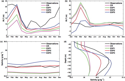
The seasonal cycle of BLT in the NWTA from observations and various experiments is shown in Fig. 13a while that in the subtropical salinity maxima region (50 W–30 W, 25 N–30 N) is shown in Fig. 13b. From these two figures, it can clearly be seen that the simulation of BLT progressively improves with each experiment. In the NWTA region, particularly the bias in simulation of BLT during late winter to early spring improves considerably and compares quite well with observations in EXP3. Similarly, the simulation of spurious BLT in the subtropical salinity maxima region during late winter to early spring in the CR is reduced substantially in EXP2 and EXP3, where we increase the surface salinity and enhance subduction. The seasonal cycle of SSS in the subtropical salinity maxima region is shown in Fig. 13c. The surface salinity in this region has a very weak seasonal cycle and this is clearly reflected in the figure. In the CR and EXP1, the surface salinity is lower than in observations by about 0.4 g kg⁻¹. The surface salinity compares quite well with observations in EXP2 while there is an overestimation in EXP3 by about 0.2 g kg⁻¹. The extent to which the model BLT in the NWTA responds to the forcing depends on the extent of model bias in the surface and subsurface. Vertical subsurface salinity profiles for the NWTA region are shown in Fig. 13d. In our present model the surface salinity bias in the NWTA region is about 0.4 g kg⁻¹. But in the subsurface, the bias is about 0.8 g kg⁻¹ at an approximate depth of 100 m. In EXP1, only the surface salinity improves as we only add a positive precipitation anomaly near the Amazon region. However in EXP2 and EXP3, the subsurface salinity improves along with the surface salinity as we enhance the subduction in the salinity maxima region.

Fig. 13.  The seasonal cycle of BLT (m) for the region averaged over (a) 65 W–50 W, 10 N–20 N and (b) 50 W–30 W, 25 N–30 N. (c) The seasonal cycle of SSS (g kg⁻¹) averaged over the region 50 W–30 W, 25 N–30 N. (d) The mean subsurface salinity averaged over the region 65 W–50 W, 10 N–20 N.

In EXP1, even though there is a shoaling of the MLD due to freshening at the surface, no temperature inversions form, as the induced salinity gradient is not strong enough to sustain an inversion. Formation of a temperature inversion requires a strong salinity gradient below the MLD, which can compensate the instability caused by an increase in temperature. Temperature inversions form in EXP2 and EXP3, as the induced salinity gradients are strong enough to sustain inversions in temperature. Also, the magnitude of temperature inversions increases with the forcing amplitude with the maximum magnitude being about 0.2 °C. Thus, to improve the simulation of temperature inversions in the model, we need to not only improve the surface but also the subsurface salinity, as both of them jointly determine the salinity stratification.

Heat budget analysis for the region of BL increase reveals that in EXP2 and EXP3, there is an increase in MLH storage rate and AHF. In the case of SHF, there is a reduction for the region of BL increase in EXP2 and EXP3. This is because the SST cooling induced by the positive E–P anomaly reinforces the easterly trades and causes an increased latent and sensible heat loss. This acts as a mechanism to damp the SST increase in the region of BL increase. Again, we do not find such a reduction in SHF in EXP1 as there is no cooling to the North to cause the changes in surface wind stress. Even though in EXP2 and EXP3, there is a slight increase in the mean THF at the mixed layer base, the signal to noise ratio is very low making it very hard to draw conclusions. Also, the THF is estimated as a residue and thus is prone to errors in approximation.

Finally, there are certain caveats in our present study. One is that the forcing is artificial. Salinity biases result not only from biases in precipitation but also from biases in wind stresses and circulation. Also in reality, the Amazon water that is discharged into the Atlantic has very high turbidity. This is due to the suspended particles found in riverine discharge. Thus it is capable of arresting the penetration of solar short wave flux and confining much of it to the very upper layers of the ocean. Because we have only changed the salinity and not the turbidity, we cannot exactly reproduce the effect of Amazon river discharge. This could be another possible reason as to why the response in SST in the region of BL increase was not very strong. The coarse resolution of the model used to conduct these experiments may also affect the sensitivity of the SST response to BL changes in the region. Future studies are needed to further investigate the potential effect of BLs on SST using improved climate models.

8. Acknowledgements

The authors wish to acknowledge use of the freely available ‘Ferret’ software for performing part of the analysis and graphics in this paper. Ferret is a product of NOAA's Pacific Marine Environmental Laboratory (information is available at http://ferret.pmel.noaa.gov/Ferret/).

References

- Antonov, J. I, Seidov, D, Boyer, T. P, Locarnini, R. A, Mishonov, A. V and co-authors. 2010. In: World Ocean Atlas 2009, Volume 2: Salinity. (S. Levitus) Vol. 69, 184 pp. NOAA Atlas NESDIS. US Government Printing Office: WashingtonDC.
- Blanke, B, Arhan, M, Lazar, A, Mignot, J and Prévost, G. 2002. A Lagrangian numerical investigation of the origins and fates of the salinity maximum water in the Atlantic. J. Geophys. Res. 107(C10), 3163. 10.3402/tellusa.v64i0.18162.
- Breugem W.-P. Chang P. Jang C. J. Mignot J. Hazeleger W. Barrier layers and tropical Atlantic SST biases in coupled GCMs. Tellus A. 2008; 60: 885–897. 10.3402/tellusa.v64i0.18162.
- Carton J. A. Zhou Z. Annual cycle of sea surface temperature in the tropical Atlantic Ocean. J. Geophys. Res. 1997; 102: 27813–27824. 10.3402/tellusa.v64i0.18162.
- Chang P. Fang Y. Saravanan R. Ji L. Seidel H. The cause of the fragile relationship between the Pacific El Niño and the Atlantic Niño. Nature. 2006; 443: 324–328. 10.3402/tellusa.v64i0.18162.
- Chang P. Ji L. Li H. A decadal climate variation in the tropical Atlantic Ocean from thermodynamic air-sea interactions. Nature. 1997; 385: 516–518. 10.3402/tellusa.v64i0.18162.
- Collins, W. D, Bitz, C. M, Blackmon, M. L, Bonan, G. B, Bretherton, C. S and co-authors. 2006. The Community Climate System Model: CCSM3. J. Clim. 19, 2122–2143.
- de Boyer Montégut, C, Mignot, J, Lazar, A and Cravatte, S. 2007. Control of salinity on the mixed layer depth in the world ocean. Part 1: general description. J. Geophys. Res. 112, C06011. 10.3402/tellusa.v64i0.18162.
- Denman K. L. A time dependent model of the upper ocean. J. Phys. Ocean. 1973; 3: 173–184.
- DeWitt, D. G. 2005. Diagnosis of the tropical Atlantic near-equatorial SST bias in a directly coupled atmosphere-ocean general circulation model. Geophys. Res. Lett. 32, L01703. 10.3402/tellusa.v64i0.18162.
- Dickinson, R. E, Oleson, K. W, Bonan, G, Hoffman, F, Thornton, P and co-authors. 2006. The Community Land Model and its climate statistics as a component of the Community Climate System Model. J. Clim. 19, 2302–2324.
- Dorman C. E. Bourke H. Precipitation over the Atlantic Ocean, 30 S to 70 N. Mon. Weather Rev. 1981; 109: 554–563.
- Emanuel K. A. Increasing destructiveness of tropical cyclones over the past 30 years. Nature. 2005; 25: 686–688. 10.3402/tellusa.v64i0.18162.
- Ffield A. Amazon and Orinoco River plumes and NBC rings: bystanders or participants in hurricane events?. J. Clim. 2007; 20: 316–333. 10.3402/tellusa.v64i0.18162.
- Foltz G. R. McPhaden M. J. Seasonal mixed layer salinity balance of the tropical North Atlantic Ocean. J. Geophys. Res. 2008; 113: C02013.10.3402/tellusa.v64i0.18162.
- Foltz G. R. McPhaden M. J. Impact of barrier layer thickness on SST in the central tropical North Atlantic. J. Clim. 2009; 22: 285–299. 10.3402/tellusa.v64i0.18162.
- Godfrey J. S. Lindstrom E. J. The heat budget of the equatorial western pacific surface mixed layer. J. Geophys. Res. 1989; 94(C6): 8007–8017. 10.3402/tellusa.v64i0.18162.
- Hazeleger W. Haarsma R.J. Sensitivity of tropical Atlantic climate to mixing in a coupled ocean-atmospheremodel. Clim. Dynam. 2005; 25: 387–399.
- Hellweger F.L. Gordon A.L. STracing Amazon river water into the Caribbean Sea. Deep-Sea Res. II. 2002; 60: 537–549. 10.3402/tellusa.v64i0.18162.
- Hu C. Montgomery E. T, Schmitt R. W. Muller-Karger F. E. Dispersal of Amazon and Orinoco River water in the tropical Atlantic and Caribbean Sea: observation from space and S-PALACE floats. Clim. Dynam. 1997; 51: 1151–1171.
- Huang B. Hu Z.-Z. Jha B. Evolution of model systematic errors in the Tropical Atlantic Basin from coupled climate hindcasts. Tellus. 2007; 28: 661–682. 10.3402/tellusa.v64i0.18162.
- Kraus E. B. Turner J. S. A one-dimensional model of the seasonal thermocline II. Rev. Geophys. 1967; 19: 98–106. 10.3402/tellusa.v64i0.18162.
- Large W. G. McWilliams J. C. Doney S. C. Oceanic vertical mixing: a review and a model with a non-local boundary layer. 1994; 385: 363–403. 10.3402/tellusa.v64i0.18162.
- Locarnini, R. A, Mishonov, A. V, Antonov, J. I, Boyer, T. P, Garcia, H. E and co-authors. 2010. In: World Ocean Atlas 2009, Volume 1: Temperature. (S. Levitus) Vol. 68, 184 pp. NOAA Atlas NESDIS. US Government Printing Office: WashingtonDC.
- Lukas R. Lindstrom E. J. The mixed layer of the Western Equatorial Pacific Ocean. Geophys. Res. Lett. 1991; 96(C6): 3343–3358.
- Maes, C, Ando, K, Delcroix, T, Kessler, W. S, McPhaden, M. J and co-authors. 2006. Observed correlation of surface salinity, temperature and barrier layer at the eastern edge of the Western Pacific warm pool. 33, L06601. 10.3402/tellusa.v64i0.18162.
- Maes, C, Picaut, J and Belamari, S. 2002. Salinity barrier layer and onset of El Niño in a coupled model. Geophys. Res. Lett. 29, 2206. 10.3402/tellusa.v64i0.18162.
- Masson S. Delecluse P. Influence of the Amazon river runoff on the tropical Atlantic. J. Geophys. Res. 2001; 26: 137–142. 10.3402/tellusa.v64i0.18162.
- Mignot, J, de Boyer Montégut, C, Lazar, A and Cravatte, S. 2007. Control of salinity on the mixed layer depth in the world ocean. Part II: tropical areas. J. Phys. Ocean. 112, C10010. 10.3402/tellusa.v64i0.18162.
- Miller J. R. The salinity effect in a mixed layer ocean model. J. Clim. 1976; 6: 29–35.
- Moisan J. R. Niiler P. P. Interaction between tropical Atlantic variability and El Niño-Southern Oscillation. J. Clim. 1998; 13: 2177–2194.
- Ohlmann J. C. Ocean radiant heating in climate models. Geophys. Res. Lett. 2003; 25: 686–688.
- Pailler K. Bourles B. Gouriou Y. The barrier layer in the western tropical Atlantic Ocean. Clim. Dynam. 1999; 26: 2069–2072. 10.3402/tellusa.v64i0.18162.
- Richter I. Xie S.-P. On the origin of equatorial Atlantic biases in coupled general circulation models. J. Clim. 2008; 31: 587–598. 10.3402/tellusa.v64i0.18162.
- Saravanan R. Chang P. Interaction between tropical Atlantic variability and El Niño-Southern Oscillation. J. Phys. Ocean. 2000; 13: 2177–2194.
- Schmitt R. W. Bogdena P. S. Dorman C. E. Evaporation minus precipitation and density fluxes for the North Atlantic. J. Clim . 1989; 19: 1208–1221.
- Smith T. M. Reynolds R. W. Improved extended reconstruction of SST (1854–1997). J. Geophys. Res. 2004; 17: 2466–2477.
- Sprintall J. Tomczak M. Evidence of the barrier layer in the surface layer of the tropics. J. Geophys. Res. 1992; 97: 7305–7316. 10.3402/tellusa.v64i0.18162.
- Vizy, E and Cook, K. 2009. Influence of the Amazon/Orinoco plume on the summertime Atlantic climate. Bull. Am. Meteor. Soc. 115, D21112. 10.3402/tellusa.v64i0.18162.
- Xie S.-P. Arkin P. A. Global precipitation: a 17-year monthly analysis based on gauge observations, satellite estimates, and numerical model outputs. Tellus A. 1997; 78: 2539–2558.
- Xie S.-P. Philander S. G. H. A coupled ocean-atmosphere model of relevance to the ITCZ in the eastern Pacific. J. Mar. Res. 1994; 46: 340–350. 10.3402/tellusa.v64i0.18162.