Dynamical system properties of an axisymmetric convective tropical cyclone model

Abstract

The dynamical system behaviour of tropical cyclones and their potential intensity with a view to sea surface temperature, tropospheric temperature stratification and tropospheric moisture content is investigated in the axisymmetric convective model HURMOD. The model results exhibit the existence of a fixed-point attractor associated with a strong tropical cyclone. Moreover, the initial vortex strength forms an amplitude threshold to cyclogenesis. Above this threshold, the size of the tropical cyclone and its intensity are independent of the initial vortex strength and its horizontal extent. Below the amplitude threshold, cyclogenesis does not occur and the system approaches an atmospheric state of rest. In case one allows for a deviation of the tropospheric stratification from moist-neutral conditions, the modelling results reveal the existence of bifurcations with the sea surface temperature representing the bifurcation parameter: As the sea surface temperature decreases and the storm weakens, the fixed-point attractor turns first into a limit cycle indicating a Hopf-bifurcation and then gives way to a steady-state of lower intensity, before the intensity oscillation becomes chaotic, and finally the tropical storm dies. The amplitude threshold and the sea surface temperature range, within which the system exhibits bifurcation points, are sensitive to the reference value of relative humidity and the reference tropospheric temperature stratification. If the reference troposphere is presumed to be moist-neutral, the dynamical behaviour of the modelled tropical cyclone does not change within the range of tropical sea surface temperature, and the tropical cyclone only slightly weakens with decreasing sea surface temperature, without any abrupt changes in intensity. Apart from the existence of Hopf-bifurcations, these findings are qualitatively similar to results gained from a low-order model presented in a precursory study.

• tropical cyclone dynamics
• potential intensity
• bifurcations
• convection-resolving model

1. Introduction

Tropical cyclones (TCs) are atmospheric low-pressure systems characterised by deep convective clouds with a vertical extent throughout the troposphere. Though it is possible to simulate TCs in numerical models quite accurately, little is known about their dynamical system characteristics. The idealised view of a TC as an autonomous dynamical system provides a useful ansatz to investigate the dynamical system behaviour of TCs by means of numerical models. Knowledge on the dynamical system properties of TCs is required to understand and judge the impact of climate change on their potential intensity (PI) and frequency of occurrence.

On the basis of extensive global observational studies of TCs and non-developing cyclonic disturbances, Gray (1979) has outlined six climatological parameters, which highly influence, whether a TC may develop or not. These genesis parameters comprise: (1) low-level relative vorticity; (2) the Coriolis parameter; (3) the inverse magnitude of ventilation controlled by the environmental vertical shear of horizontal wind between the lower and upper troposphere; (4) ocean thermal energy as reflected by the sea surface temperature (SST) excess above 26°C in a layer of at least 60 m depth; (5) the vertical gradient of equivalent potential temperature in the lower and mid-troposphere as a criterion for convective instability; and (6) environmental relative humidity at mid-tropospheric levels. As pointed out by Ooyama (1982), the synoptic and thermodynamic environmental conditions do not directly determine the process of cyclogenesis, but influence its probability, and in turn the frequency of occurrence of TCs. It has been hypothesised by Emanuel and Nolan that TCs can be understood as a stable branch occurring beyond a subcritical saddle node bifurcation at a certain SST. The other unstable branch after the bifurcation is associated with smaller but finite wind speeds that must be exceeded initially for the excitation of tropical cyclogenesis. Therefore, it can explain why not all initial perturbations develop into TCs. It remains to be further investigated, why such a bifurcation should occur and what physical processes are responsible for this.

Tang and Emanuel (2010) have shown that entrainment of low-entropy air due to vertical wind shear towards the centre may form an obstruction to TC formation and intensification. This confirms and explains the relevance of one of the Gray genesis parameters. In a conceptual model, they found a ventilation threshold, i.e. a bifurcation. Further evidence for the existence of such a threshold is given in their follow-up study (Tang and Emanuel, 2012), where they show that the bifurcation is also visible in a non-hydrostatic axisymmetric convective model. Emanuel (1989) demonstrated with a simplified axisymmetric model that the import of low-entropy air into the boundary layer by shallow clouds or precipitation-induced downdrafts can provide reasons for the finite amplitude nature of tropical cyclogenesis. On the basis of more complex models, Frisius and Hasselbeck (2009) showed that precipitating downdrafts are chiefly responsible for the suppression of initial perturbations. Therefore, it is likely that such processes are an essential ingredient to reproduce dynamical system characteristics of a TC in numeric models that are closer to those of a real TC. Furthermore, Swanson (2008) found in an analysis of observational data that the intensity and overall activity of TCs in response to changes in the SST exhibits a highly non-local character. This means that seasonal tropical cyclone activity in a certain basin does not only depend on local SST changes within the respective main development region but is correlated to the relative SST (i.e. local minus tropical-mean SST), since the free-tropospheric temperatures at higher levels tend to follow tropical-mean SSTs (Zhao et al., 2009; Yu et al., 2010; Camargo et al., 2013). This suggests that besides the local SST, also the tropospheric temperature stratification, as well as upper-level tropospheric temperatures play a crucial role in tropical cyclone system dynamics.

In a precursory study, a conceptual model has been developed (Schönemann and Frisius, 2012). Its results showed a strong quantitative and qualitative sensitivity of equilibrium states to thermodynamic environmental control parameters. These include the SST, the vertical temperature stratification and the moisture content of the troposphere. For tropical ocean parameter settings the low-order model possesses up to four equilibria, which arise as a result of a subcritical bifurcation at a certain critical SST, and a cusp catastrophe at a higher SST, where the stable branch splits into one unstable and two stable equilibria. This consistently explains the rise of TC intensity with increasing SST as well as the suppression of tropical cyclogenesis at low SSTs and in an insufficiently moist environment. However, in the conceptual model, a number of processes relevant to the dynamics of TCs, some already mentioned above, are largely parameterised by relatively simple relations. In order to be able to further specify and capture physical processes on smaller scales, such as convective and turbulent exchange, a rather complex cloud-resolving model is required. For this reason, investigation of the sensitivity of PI and the bifurcation structure in terms of the respective thermodynamic parameters will be also performed with the high-resolution axisymmetric convective model HURMOD (Frisius and Wacker, 2007; Frisius and Hasselbeck, 2009). In that sense, the study at hand ties in with the investigation of TC dynamics within a conceptual model by Schönemann and Frisius (2012).

The remainder of this study is organised as follows: A brief introduction to the cloud-model HURMOD and the parameterisation of subscale processes applied in this study is provided in Section 2. Section 3 gives an overview over the model experiments, and modelling assumptions and approximations that are made in the framework of the long-term simulations with HURMOD. In Section 4, the parameter sensitivity and the dynamical system behaviour of the convective model HURMOD are investigated and discussed. A discussion on the results from HURMOD in comparison to the results from the low-order model (Schönemann and Frisius, 2012) is given in Section 5. A summary containing concluding remarks is given in Section 6.

2. Model description

For our numerical experiments, we use the cloud-resolving atmospheric model HURMOD, which is designed to capture convective motion in detail. HURMOD is formulated in cylindrical coordinates (r,ϕ,z) on the basis of the approximation of an axisymmetric vortex flow, which is suitable to simulate the inner dynamics of TCs. The spatial dependence of the Coriolis acceleration is neglected, and a constant value corresponding to that at a latitude of 20° is taken for the whole model domain. Similar models have been developed and introduced in several previous studies [e.g. Willoughby et al. (1984), Rotunno and Emanuel (1987), Bryan and Fritsch (2002), Tang and Emanuel (2012)]. All quantities are computed on a staggered Arakawa-C-type grid as in Rotunno and Emanuel (1987). The cylindrical model domain has a vertical extent of 20 km and a radius of 2000 km. The vertical grid spacing is Δz=250 m, and the radial grid spacing in the centre within a radius of 120 km is Δr=500 m, rising non-linearly with radial distance to the centre to in the outermost ring of the model domain. For time integration, we employ a leap-frog scheme. An extensive description of the model is given in Frisius and Wacker (2007). A brief description of the model and the parameterisation used in this study will be given in the following subsections. Further approximations and the initial conditions are outlined in Section 3.

2.1. Prognostic equations

The governing equations are phrased in flux form. In comparison to the advective form, the flux form is more suitable to avoid non-physical sources and sinks and, therefore, improves the computation of conserved properties. The prognostic variables in the equations of motion are radial, tangential and vertical momentum density (ρu, ρv and ρw). The momentum equations are given by:1 2 3

where the potential temperature θ, the mass fraction of water vapour q _v and the non-dimensional pressure ∏ (also referred to as the Exner function), can be split into their horizontally independent reference value, denoted by the index 0, and the deviation from the respective reference state, denoted by an asterisk. The continuity equation is given by:4

the temperature equation is formulated in terms of the potential temperature flux:5

and the budget equations for water vapour (index v), cloud water (index c) and rain water (index r) are given by:6 7 8

The first and second terms on the rhs of the prognostic eqs. (1)–(8) represent the advection of the respective variable. In the computation of the horizontal momentum fluxes (1)–(2), Coriolis and centrifugal forces are accounted for by the third term on the rhs. The radial and vertical components of the pressure gradient are represented by the fourth term on the rhs of eq. (1) and the third term on the rhs of eq. (3), respectively. The effect of buoyancy is given by the fourth term in the vertical momentum eq. (3). In all of the equations above, the exchange through micro-turbulent mixing of the respective variable G is denoted by D _ρG . In the temperature eq. (5), heat fluxes via radiative cooling and dissipative heating via turbulent eddies are described by the third term, and latent heat and vertical diffusive mass fluxes (J _G ) are represented by the fourth term on the rhs. In eqs. (6)–(8), Q _v , Q _c and Q _r denote sources and sinks for the respective substance related to transition processes (i.e. condensation, evaporation, autoconversion, coalescence), and vertical diffusive fluxes are represented by the fourth term on the rhs. An overview over the model variables and constants in the governing equations is provided in Table 1.

Table 1. Notations for variables and constants in prognostic equations (1)–(8)

Notation	Value	Meaning
t	Time
r	Radius
z	Height
u	Radial velocity
v	Tangential velocity
w	Vertical velocity
V	Horizontal wind speed
Π	Non-dimensional pressure (Exner function)
ρ	Air density
T	Absolute temperature
θ	Potential temperature
q v	Mass fraction of water vapour
q c	Mass fraction of cloud water
q r	Mass fraction of rain water
J G	Vertical diffusive mass flux of substance G
(G=dry air, water vapour, cloud water, rain water)
Φ	Dissipation rate
Q R	Radiative heating rate
D ρG	Micro-turbulent flux of quantity G
(G=u,v,w,θ,q v ,q c ,q r )
c p	Specific heat capacity of air at constant pressure
c pd	1005 Jkg ^−1 K ^−1	Spec. heat capacity of dry air
c pv	1848 Jkg ^−1 K ^−1	Spec. heat capacity of water vapour
c pl	4185 Jkg ^−1 K ^−1	Spec. heat capacity of liquid water
R d	287.0 Jkg ^−1 K ^−1	Spec. gas constant of dry air
R v	461.5 Jkg ^−1 K ^−1	Spec. gas constant of water vapour
l v	2.5·10^−6 Jkg ^−1	Latent heat of vapourisation
f	5·10^−5 s ^−1	Coriolis parameter
g	9.81 ms^−2	Gravitational acceleration

2.2. Parameterisation of subscale processes

The parameterisation of turbulent mixing by small-scale eddies follows the commonly used simple K-ansatz, where turbulent fluxes are described in analogy to molecular diffusion, and are assumed to be proportional to a parameterised eddy-diffusivity K. The eddy-coefficient K is assumed to be equal for turbulent exchange of momentum and energy, but we distinguish between vertical and horizontal eddy-diffusivity, K _v and K _h respectively. The diagnostic calculation of K _v and K _h follows that by Bryan and Rotunno (2009c) [cf. their eq. (16) and (17)]. As HURMOD is formulated in flux form in this study, we use dynamic instead of kinematic diffusivity:9

where denotes vertical and horizontal strain deformation, N is the Brunt-Väisälä or stability frequency, and l _h and l _v represent the horizontal and vertical mixing length scale, respectively. The eddy-diffusivity formulated in eq. (9) is proportional to the squared mixing length scale, which has to be parameterised. In a modelling study, Bryan and Rotunno (2009c) find that TC intensity exhibits a considerable sensitivity to l _h . They suggest a value of l _h =1500 m to be reasonable. Here, we take a lower value of l _h =750 m, which was derived by Zhang and Montgomery (2012) based on in situ aircraft measurements taken in the boundary layer of three strong hurricanes.

Bryan and Rotunno (2009c) also show that the shape of the horizontal flow field in and near the eyewall region is strongly influenced by the choice of l _v [cf. their Fig. 5]. In a test study on boundary layer schemes and their turbulence parameterisation, Kepert (2012) argues that biases in the lowest model level flow, thermodynamic fields, and consequently in the surface fluxes occur due to an overestimation of eddy-diffusivity at the lowest model level in many Bulk schemes, when the mixing length is treated as a spatially independent constant. As recommended by Kepert (2012), we implement a height-dependent formula to calculate the vertical mixing length l _v , developed 50 years earlier by Blackadar (1962) [cf. his eq. (24)]:10

where k is the von Kármán-constant, and is the value of l _v at infinite height. For and with k=0.4, we obtain l _v =100 m at z=500 m. This agrees with the value derived by Zhang et al. (2011) from aircraft data collected in the eyewall region of one category 4, and one category 5 hurricane.

The computation of micro-turbulent atmosphere–ocean exchange is based on a commonly used bulk algorithm [cf. eq. (20) in Frisius and Hasselbeck (2009)]. In the study at hand, vertical turbulent surface fluxes are calculated as a function of the horizontal wind speed V _10m at z=10m instead of that at the lowest model level11

where G ₀ represents the value of water vapour, heat or momentum at z=0 m, and C _G is the surface transfer coefficient of the respective quantity G. Both the radial and tangential component of V _10m is approximated by assuming a logarithmic wind profile beneath the lowest model level12

where V _10m represents either the radial (u _10m) or the tangential wind velocity (v _10m) at z=10 m, V ₁ the corresponding component of the horizontal wind velocity at the lowest model level above the sea surface, z ₁, and r _L the sea surface roughness length. The roughness length r _L is a function of the surface exchange coefficient for momentum C _D (usually referred to as drag coefficient) and calculated at z=10 m:13

In several previous TC modelling studies, both the drag coefficient C _D and the surface exchange coefficient for heat and moisture C _H are chosen to be equal and are prescribed as a linear function of horizontal wind speed V at a near-surface level according to Deacon's formula [e.g. Rotunno and Emanuel (1987), Frisius and Hasselbeck (2009)]. Instead of using Deacon's formula, the surface exchange coefficients will be determined in close agreement with the results from observation-based studies by Black et al. (2007) and Fairall et al. (2003). For C _H we take a constant value of 1.2·10⁻³, which is very close to the value found by Black et al. (2007) (cf. their Fig. 6). The drag coefficient is assumed to vary linearly with wind speed within a certain range of V _10m [cf. Fig. 5 in Black et al. (2007) and Fig. 10 in Fairall et al. (2003)]:14

As the drag coefficient C _D by itself is a function of wind speed V _10m we only iteratively compute proximate solutions to eqs. (12)–(14). Notwithstanding, it is probably much more realistic to calculate the turbulent surface exchange [eq. (11)] on the basis of 10 m-wind speeds rather than that at the much higher first model level, which would possibly result in an excessive inflow and, consequently, a stronger updraught (Kepert, 2010).

The effect of radiation is parameterised in a most simplistic manner by application of a so-called ‘Newtonian cooling’ (Rotunno and Emanuel, 1987), given by15

where τ _R is a time scale for radiative cooling, and θ _E denotes the radiative equilibrium potential temperature (for further notations, see Table 1). In HURMOD, τ _R is set to 12 h, and θ _E is assumed to be equal to the potential temperature of the reference state θ ₀. Therefore, the Newtonian cooling can be viewed as a radiative damping or relaxation of the potential temperature field. Where other processes that affect the temperature, such as advection or turbulent mixing, become negligible, Newtonian cooling is dominant and acts to relax the temperature to its initial vertical profile.

3. Experimental set-up

The sensitivity experiments are grouped into two sets: One, which allows for both moist stability and instability, and another one, where the tropospheric stratification is kept moist-neutral. The first set-up corresponds to the non-neutral case I considered in the low-order model introduced by Schönemann and Frisius (2012), and the second set to the moist-neutral case N. To realise case N in HURMOD, the tropospheric equivalent potential reference temperature above the surface layer is kept vertically constant by an iterative adjustment of temperature and specific humidity. The tropospheric relative humidity and specific humidity as well as temperature at the lowest model level are not altered in this procedure. In case I, the tropopause temperature is taken as a reference parameter, and the lapse rate is adjusted according to the prescribed SST-value and the respective reference tropopause temperature value. In addition to this, some simulations are carried out in which the temperature lapse rate serves as a reference parameter, and the tropopause temperature is adjusted accordingly. The latter set of model experiments will be referred to as case J. In both case I and J, the vertical reference temperature profile is presumed to be simply linear throughout the troposphere, and hence the environmental (or reference) tropospheric lapse rate is equal to the difference between the SST and the reference tropopause temperature, divided by the tropopause height. As long as the far-field is calm so that dynamical processes do not play a role, the temperature profile is fixed in accordance with the initial boundary conditions via radiative forcing. For all three cases, the reference value of the tropopause height, z _t , is set to 15 km. Regarding the initial relative humidity, RH _ref , we choose a highly idealised set-up, where RH _ref is presumed to be distributed homogeneously throughout the troposphere and to decrease linearly from above the tropopause to zero at the upper vertical boundary of the model domain. The main distinguishing features between these three sets are listed in Table 2.

Table 2. Characteristics of different experimental set-ups in HURMOD

Designation	Moist stability	Reference stratification
Case I	Non-neutral	Time-invariant tropopause temperature T t
Case J	Non-neutral	Time-invariant tropospheric lapse rate Γ
Case N	Moist-neutral

In the standard configuration, the cyclones are initialised with a SST of T _s=30°C, a tropospheric relative humidity of RH _ref =70%, a tropopause temperature of T _t =−70°C in case I, which corresponds to a temperature lapse rate of which is also applied in case J, a minimum surface pressure of 1005 hPa in the centre of the model domain, and an environmental reference surface pressure of p ₀₀=1015 hPa. Within a radius of twice the initial RMW, the initial disturbance has the shape of a modified Rankine vortex (Holland, 1980). Further outward, the tangential wind at the lowest model level is assumed to decay continuously faster with increasing radius as proposed by George Bryan (personal communication):16

with

where r ₀ is the radius of vanishing wind, and the index init has been omitted. If not stated otherwise, the initial radius of maximum wind (RMW _init ) is situated at a distance of 100 km from the centre and the initial radius of vanishing lowest-level winds (r _0,init ) at a radius of 500 km. The vertical distribution of the initial wind field is calculated as follows:17

where z _t denotes the tropopause height, which is set to 15 km (see above). We presume the initial state to be in gradient wind and hydrostatic balance to relate the initial pressure anomaly to the initial tangential velocity field as given by eqs. (16)–(17). With this and the respective moisture and temperature reference profiles, the initial Π- and θ-anomalies can be determined numerically.

First, the steady-state sensitivity to the initial vortex size in the standard configuration is investigated for case I. Then, in both configurations, non-neutral case I and moist-neutral case N, we run long-term model experiments over a modelling period of 4000 h (i.e. almost 7 weeks). The choice of the integration time for the long-term simulations is entirely based on practical considerations. It has been found in numerous model experiments that the system reveals its final character after a shorter period of time than 4000 h; i.e. the system either approaches a steady-state, which resembles the behaviour of a fixed-point attractor corresponding to a stable equilibrium for rather intense model storms, or a lower steady-state with small but visible intensity oscillations, or a state of rest. This behaviour will be illustrated and discussed in the subsequent sections of this study. The simulations are carried out with different values for SST and initial tropospheric relative humidity to test the sensitivity of TC intensity and size to SST and atmospheric moisture content. Note, the SST represents a lower boundary condition in HURMOD. Hence the ocean is considered as an unlimited energy reservoir, whereas the air–sea interaction associated with real TCs results in a cooling of surface waters beneath the TC due to enhanced vertical turbulent entropy fluxes into the atmosphere, vertical turbulent mixing within the ocean mixed layer and upwelling (Knaff et al., 2013; Mei and Pasquero, 2013). In case I, we also run simulations with different values for the tropopause temperature to test the sensitivity to vertical temperature stratification and outflow temperature. In a second step, we investigate the cyclone behaviour in response to slow changes in SST for all three cases listed in Table 2 and for three differing configurations in case I. These simulations are started from a stable state and are run with a linearly decreasing SST at a rate of 0.001°C/h. The dynamical behaviour in the standard configuration of case I will be outlined in further detail.

For the purpose of long-term model experiments to achieve a stable state, the simulations are run in the hydrostatic mode. This allows us to apply a considerably larger time-step (Δt=1s−2s) compared to that required in the non-hydrostatic configuration (Δt=0.16s−0.32s) and thus to reduce computational costs by a factor higher than six. In order to roughly mimic the effect of moisture exchange through the lateral boundary, without introducing artificial lateral gradients in the moisture field, a global relaxation of the moisture field is applied in an analogue way to the Newtonian cooling. We assume that the relaxation rate for moisture (τ _Q =120 h) is by one order of magnitude slower than that for radiative cooling (τ _R =12 h). Furthermore, the virtual temperature correction is neglected, and consequently, the buoyancy term in eq. (3) simplifies to:18

By application of the global moisture relaxation and neglecting the virtual temperature correction, the long-term development of artificial disturbances at the closed lateral boundary can be avoided.

4. Results

4.1. Initial vortex size

In order to test the sensitivity to a given initial size of the disturbance, we performed long-term simulations with four different initial values of the RMW, and correspondingly four different values in the initial radius of vanishing surface wind speed, r _0,init (RMW _init =50 km & r _0,init =250 km; RMW _init =100 km & r _0,init =500 km; RMW _init =150 km & r _0,init =750 km; RMW _init =200 km & r _0,init =1000 km). 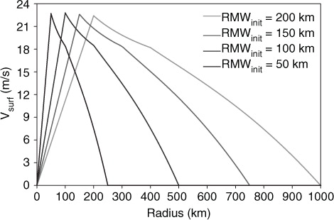The maximum wind speed of the initial vortex, v _max,init , is chosen to be in this set of experiments. The initial tangential wind profiles at the lowest model level according to eq. (16) are displayed in Fig. 1. Whether cyclogenesis occurs or not, may also depend on the initial vortex strength as will be depicted later on in Section 4.2.

Fig. 1 Initial tangential surface velocity as a function of radial distance to the centre for four different values in the initial RMW (50 km, 100 km, 150 km, 200 km).

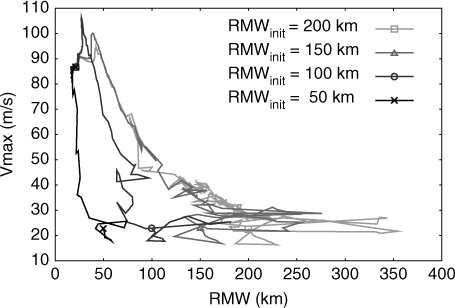
The trajectories in the phase diagram spanned by the RMW and the maximum wind speed (Fig. 2) reveal that a TC attractor exists in HURMOD. The TC reaches an equilibrium, where both RMW and maximum horizontal wind speed are independent of the initial perturbation radius as can be seen in Fig. 2. For the standard configuration in case I, we obtain an equilibrium at a maximum horizontal wind speed of ~87 m/s at a radius of ~21 km. At first glance, this result appears to disagree with what was indicated by Rotunno and Emanuel (1987) and confirmed by Xu and Wang (2010). The output from the numerical study by (Rotunno and Emanuel, 1987) gave evidence suggesting that there is a slight dependence of TC intensity in the mature stage with regard to the initial vortex size and that the initial size of a TC largely determines its final size. Further evidence for this behaviour is given by Xu and Wang (2010), whose 3-D model simulations also show that cyclones that stem from an initially larger disturbance remain larger than those originating from a spatially rather small initial disturbance. However, we note, the larger the initial extent and the further outward away from its equilibrium position the initial radius of maximum wind is, the longer it takes until the stable equilibrium state is reached. Over a shorter time period of the first 10 days, we also observe that storms with an initially larger RMW keep a larger extent than those started from a smaller RMW. In this respect, the results from HURMOD are in qualitative agreement with the findings by Rotunno and Emanuel (1987) and Xu and Wang (2010). Presumably, there also exists a lower and an upper threshold for the size of the initial disturbance to form a TC in HURMOD. However, within the range of the spatial extent for the initial vortex investigated here, all disturbances develop sooner or later into a TC.

Fig. 2 Trajectories in a phase diagram spanned by maximum horizontal wind speed and RMW for different initial RMW values (50 km, 100 km, 150 km, 200 km). A marker is plotted at the starting point (t=0 h) and the final point (t=4000 h) on each trajectory.

4.2. Environmental relative humidity and temperature stratification

To investigate the sensitivity of TCs to environmental moisture content, we have run simulations for case I and the moist-neutral case N with an initial tropospheric relative humidity of RH _ref =50%, 60%, 70%, and 80%, respectively. In the final stage, the TCs have a similar structure, but differ in their spatial extent and in vortex strength. Radial–vertical profiles of relative humidity and radial velocity for two different values in RH _ref for case N and case I are displayed in Fig. 3. Outside the storm core, a relatively dry region forms above the boundary layer at mid-tropospheric levels. Further outward in the far-field environment, relative humidity becomes approximately uniform in the horizontal plane and increases with height to form a stratus cloud at upper tropospheric levels.

Fig. 3 Radial velocity (contour lines) and relative humidity (shadings) fields for two different values in initial tropospheric relative humidity: RH _ref =70% in the upper panels (a) and (b), and RH _ref =50% in the lower panels (c) and (d). Stable state results averaged over the last 120 h for case N are displayed on the left, and those for case I on the right.

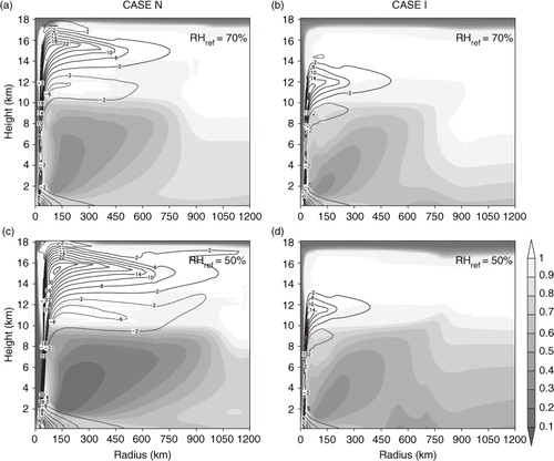
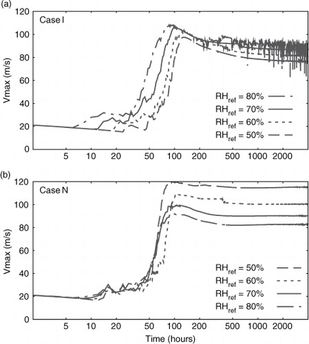
As can be seen in Figs. 3 and 4, case N and case I show a contrasting behaviour in response to different values in RH _ref . In case N, the TC becomes stronger (i.e. more intense) and more spacious with decreasing RH _ref , whereas in case I the trend is vice-versa. It can also be seen that the sensitivity of the intensity to RH _ref is stronger in case N than in case I. The latter result is closer to findings by Wang (2009) and Hill and Lackmann (2009). Both studies detected a rather weak dependence of storm intensity with regard to environmental relative humidity in 3-D model simulations. Moreover, the sensitivity of TC size to RH _ref in case I corresponds with results from the modelling study by Hill and Lackmann (2009), who found that the lateral extent of TCs increases with increasing environmental moisture content. As pointed out by Gray (1979), an enhanced relative humidity at mid-tropospheric levels is favourable to the formation of TCs and, hence, expected to be a determining factor with regard to their frequency of occurrence. This is partially confirmed by a more recent modelling study of Zhao and Held (2012). According to their results, mid-tropospheric relative humidity and TC frequency are strongly correlated in all ocean basins, expect the South Pacific. This suggests that the case I scenario is more realistic than the case N scenario. For RH _ref =80% in case I, no equilibrium is reached. Instead, high-frequency fluctuations occur, which are related to convection in the ambient region. For this scenario, the reference troposphere becomes unstable giving rise to convective bursts in the ambient region, which act to disturb the flow within the TC thereby diminishing its intensity. In both case I and N, the relative humidity under the eyewall in the final stage appears to be correlated to RH _ref , i.e. the higher RH _ref , the higher RH under the eyewall. For a 10%-change in RH _ref , we obtain a difference of ~1% at the lowest model level beneath the eyewall (not shown). Camp and Montgomery (2001) found a similar sensitivity with regard to RH beneath the eyewall for the Emanuel-model to that we see in case N, whereas case I displays a RH-sensitivity rather similar to that found by Holland [cf. Fig. 1 in Camp and Montgomery (2001)].

Fig. 4 Time development of maximum horizontal wind speed for (a) case I with a constant equilibrium tropopause temperature of T _s=−70°C and (b) the moist-neutral case N, in simulations with differing parameter values for the reference relative humidity, RH _ref . Note: The time scale is logarithmic.

In the case I scenario in HURMOD, the sensitivity of TC intensity to RH _ref is rather low compared to that in case N (Fig. 4). On the other hand, the sensitivity of the amplitude threshold, which appears in the non-neutral case I (and J), is quite high. This becomes evident from simulations with different initial vortex strength given by the initial central surface pressure difference, Δp _init , between the core and the environment (Fig. 5). For RH _ref =70% (Fig. 5a), even very weak cyclonic disturbances with a central surface pressure reduction of only 200 Pa develop into a TC, whereas for RH _ref =50% (Fig. 5b), an initial pressure reduction of ~1000 Pa is required to finally reach the TC state. From this we would expect that environmental relative humidity has a considerable impact on the frequency of occurrence of TCs. This also agrees with findings from recent observational data over the Bay of Bengal (Yanase et al., 2012).

Fig. 5 Time development of maximum horizontal wind speed in case I, for varying initial vortex strength given by the initial central surface pressure difference, Δp _init , between the core and the environment in simulations with differing parameter values for the reference relative humidity, RH _ref , and the tropopause temperature, T _t , from top to bottom: (a) RH _ref =70% and T _t =−70°C, (b) RH _ref =50% and T _t =−70°C, and (c) RH _ref =70% and T _t =−60°C. Initial disturbances that reach TC strength are displayed by black lines, non-developing systems by grey lines.

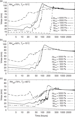
The results from HURMOD simulations also show that tropospheric dry static stability plays a certain role with regard to the frequency of occurrence of TCs, but primarily it appears to have a strong impact on TC intensity. This can be seen by comparison of Fig. 5a and Fig. 5c, and in Fig. 6. The latter shows the evolution of TCs for four different values in the reference tropopause temperature in the case I scenario. As mentioned in Section 3, in all case I and J simulations, the reference temperature profile is assumed to be linear, i.e. altering the environmental T _t at a constant SST implies a change in dry static stability. If we lower the dry static stability by increasing the tropopause temperature by 5°C within the range of −70°C≤T _t ≤−60°C, and T _s=30°C, the maximum wind speed decreases by 14–15 m/s (Fig. 6). For an even lower tropopause temperature of T _s=−75°C, the reference troposphere becomes unstable and fluctuations in the flow field occur, which are similar to those, we obtain for RH _ref =80% (see above). However, as long as the troposphere in the ambient region does not become statically unstable, our results show that the lower the static stability, the higher is the intensity of the storm and the lower is the amplitude threshold. This is in agreement with results from previous studies based on observations over different ocean basins (Zeng et al., 2008; Wada et al., 2012). Wada et al. (2012) pointed out that the relatively low static stability over the western Pacific compared to that over the eastern Pacific is a relevant factor to explain why TCs are stronger over the western than over the eastern Pacific.

Fig. 6 Time development of maximum horizontal wind speed for case I in simulations with differing parameter values for the tropopause temperature, T _t .

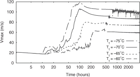
Moreover, both observation and modelling-based studies (Zeng et al., 2008; Yu et al., 2010) confirm that the outflow temperature at upper tropospheric levels is an important factor with regard to PI, as anticipated in earlier theoretical studies, based on the description of the energy cycle of a TC in analogy to that of a Carnot heat engine (Emanuel, 1986, 1995; Bister and Emanuel, 1998). In this view, the thermodynamic efficiency of the system is a function of the difference between the inflow-temperature near the surface and the outflow temperature in the upper troposphere. Changes in the tropopause temperature are also reflected in the outflow temperature of the storm at upper tropospheric levels. As the vertical extent varies with the intensity in HURMOD, we estimate the outflow temperature T _out by assuming that it corresponds approximately to the temperature at the point, where the radial velocity reaches 2 m/s at the outermost location in the outflow layer. By comparison of the simulations shown in Fig. 6 with T _t equal to −60°C, −65°C and −70°C, respectively, we find that a drop of 5°C in T _t in the ambient region corresponds to a drop of about 7°C in T _out (not shown). Hence, the colder T _t , the colder becomes T _out , so that the thermodynamic efficiency rises, and, as expected, the TC becomes more intense.

This may also provide an explanation for the behaviour, we obtain in case N with regard to the reference value of relative humidity. As discussed above, the sensitivity to RH _ref in the non-neutral case is opposite to that found in case I. This is due to the moist-neutral adjustment, which results in colder temperatures in the outflow region at upper tropospheric levels for a drier reference troposphere. Thus, the lower RH _ref , the higher becomes the thermodynamic efficiency (and vice-versa) in case N. Furthermore, the moist-neutral adjustment leads to a slightly higher efficiency at lower SSTs, i.e. the weakening effect of sea surface cooling may be partially offset by an enhanced thermodynamic efficiency, providing a possible explanation for the relatively low sensitivity of the intensity to the SST in case N, which will be displayed in the following subsection (cf. Fig. 7).

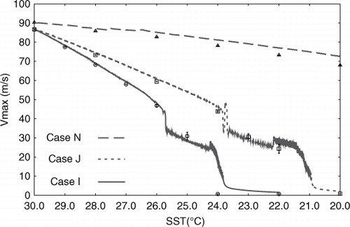
Fig. 7 Development of maximum horizontal wind speed with decreasing SST with time at a cooling rate of 10⁻³°C/h for the moist-neutral case N (dashed line), case J with Γ=const (dotted line) and case I with T _t =const (solid line). Average values over the last 120 h of the 4000 h-runs at fixed SSTs are plotted with different markers for case N (triangles), case J (squares) and case I (circles). Error bars display the full range of maximum wind speed during the last 120 h of the long-term runs.

4.3. Dynamical system properties

The dynamical behaviour of the vortex in response to changes in the SST, depends on whether the tropospheric reference state is chosen to be moist-neutral (case N) or not (case I and J). This becomes evident from simulations, which are started from a stable state with T _s=30°C, and exposed to a very slow surface temperature cooling at a rate of 10⁻³°C/h, until either an SST of 20°C is reached, or an SST, where the storm dies off (Fig. 7). Additionally, we have run long-term simulations at different constant SSTs in order to assure that the results from the cooling experiments are not chiefly due to transient dynamics related to the continuous changes in SST. As can be seen in Fig. 7, we obtain only little sensitivity to the SST in case N, where the maximum sustained winds in the eyewall decrease only slightly at colder SSTs. In contrast, the non-neutral case I and J deliver a generally higher sensitivity to SST as well as rather sudden changes in V _max , which point to the existence of bifurcation points.

Case I and case J behave qualitatively very similar, but differ quantitatively in their dependence on the SST. For our standard configuration with T _s=−70°C and RH _ref =70%, case I weakens faster with decreasing SST than case J, where the far-field temperature lapse rate is held constant at . The first jump in vortex intensity occurs at in case I, and at in case J. One can also see that the storm entirely decays at SSTs close to 24°C in case I, whereas in case J we still obtain quasi-steady-state vortices of tropical storm intensity at SSTs near 22°C. We note, unlike in the other long-term experiments displayed in Fig. 7, a stable equilibrium is not reached after 4000 h in the case J run with a constant SST of 22°C (not shown here). In this experiment, a maximum horizontal wind speed of ~28 m/s is reached after 2 days, which then slightly decreases, re-intensifies and then fluctuates between ~27 m/s and ~34 m/s for several days, after which fluctuations become small and the storm continuously weakens to V _max ~25 m/s, before it starts to oscillate again (after about 50 days of running time), with a very slow decreasing trend, and increasing amplitudes in the fluctuations. If we ran this simulation for even longer, we would expect the storm to slowly decrease further, until it finally decomposes and the atmosphere approaches a state of rest. A similar behaviour is also reflected in the cooling experiment.

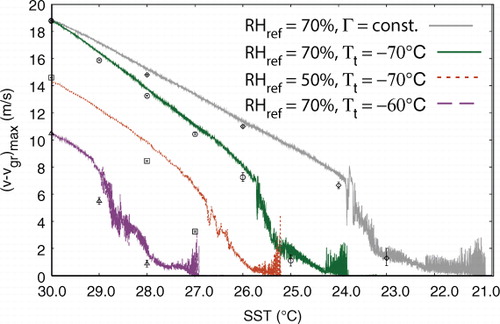
Recalling the results shown in Section 4.2, the quantitative differences in case I and case J can be simply attributed to the difference in their static stability, and outflow temperatures, which arises between these two cases when the SST is changed. In the cooling experiments shown here, the reference temperature lapse rate is continuously decreased in case I and kept constant in case J, which affects the PI via a higher or lower dry static stability, and thermodynamic efficiency as discussed in the previous section (cf. Fig. 6). A comparison of different cooling experiments in case I, further evinces the relevance of the tropospheric temperature stratification. The maximum horizontal wind speed in response to surface cooling for three different settings regarding tropopause temperature and reference relative humidity are shown in Fig. 8. The weakening rate of the vortex in the strong TC state appears to be similar and independent of the tropospheric reference state. On the other hand, the SST at which a rapid weakening takes place and that below which the storm decays completely are strongly sensitive to the thermodynamic reference conditions, especially to the tropopause temperature.

Fig. 8 Development of maximum horizontal wind speed with decreasing SST with time at a cooling rate of 10⁻³°C/h in case I for three simulations with differing parameter values for the reference relative humidity, RH _ref , and the tropopause temperature, T _t . Average values over the last 120 h of the 4000 h-runs at fixed SSTs are plotted with different markers for RH _ref =70% and T _t =−70°C (circles), RH _ref =50% and T _t =−70°C (squares), and RH _ref =70% and T _t =−60°C (triangles). Error bars display the full range of maximum wind speed during the last 120 h of the long-term runs.

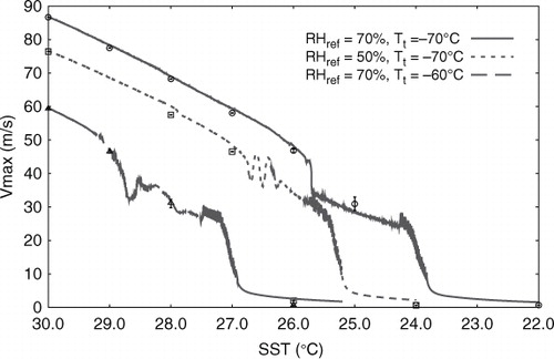
The jump in maximum wind speed appears to be most pronounced or abrupt in the reference run, displayed by a solid line in Fig. 8. For a drier reference atmosphere (RH _ref =50%), displayed by a dotted line, the cyclone displays vacillations between the high-intensity and the low-intensity state within a small SST range, before it settles into the lower TC state. In a run with a higher cooling rate (not shown), similar vacillations appear, and one vacillation also occurs in the cooling experiment for case J (see Fig. 7, dotted line). In the SST range between the first drop in maximum wind speed and before the decay of the cyclone, the surface cooling experiment with a warmer tropopause (T _t=−60°C), displayed by a dashed line in Fig. 8, does not exhibit such a monotonous, relatively smooth decrease in V _max as the standard run (T _t=−70°C), nor do we see rather rapid fluctuations between a strong TC state with V _max ≥44 m/s and, following the classification according to the Saffir-Simpson hurricane scale (SSHS), a tropical storm or relatively weak TC state with V _max ≤35 m/s as in case J. However, if we compare the quasi-steady-state obtained from long-term runs at a fix SST with T _s=26°C for the standard experiment, and T _s=28°C for the experiment with T _t=−60°C in case I, and with T _s=23°C in case J, we find that they are almost identical, in terms of final intensity (see Figs. 7 and 8) and spatial extent (not shown). The mean value of V _max is close to 31 m/s and slightly fluctuates by an amount of ~1–1.5 m/s around its mean value in both experiments. Overall, this gives rise to the assumption that the principal equilibrium structure in case I and J is, at least within a certain parameter range, fairly robust to changes in the reference lapse rate. For drier initial conditions, the SST range within which a lower equilibrium corresponding to a weak TC exists, appears to narrow. In the simulation with RH _ref =50%, the equilibrium solution representing the strong TC state may either vanish or the attractor may possibly turn directly into a repellor at a certain SST between 27°C and 26°C, so that the TC quenches off instead of first experiencing a transition to some lower or second stable state before it decomposes.

To investigate the behaviour and the character of the bifurcation in the range, where the transition from a strong TC state to a rather weak TC state takes place in more detail, we carried out another sea surface-cooling and a warming experiment with the standard configuration in case I (RH _ref =70%, T _t =−70°C). The result for SSTs between 26.6°C and 25°C is shown in Fig. 9. Here, we applied a very low cooling (warming) rate of 2·10⁻⁴°C/h to further reduce effects related to transient rather than to steady-state behaviour. The warming experiment (brighter grey line) was started from a 4000 h-run with T _s=25°C, and the cooling experiment (dark grey line) from the stable state of the 4000 h-run at T _s=27°C. In the cooling experiment, the decrease in V _max with declining SST is smooth for T _s≥26.2°C. At slightly colder SSTs, the decreasing trend persists, but V _max starts to fluctuate irregularly. The amplitude of these chaotic fluctuations rises with decreasing SST until an abrupt decrease in V _max between 25.9°C and 25.8°C occurs, where V _max drops from ~45 m/s to ~32 m/s. As the SST is further cooled down, V _max fluctuates again, but stays below 38 m/s with a slightly decreasing trend. The warming experiment displays irregular fluctuations with a maximum amplitude of ~3 m/s near T _s=25°C, and an increasing trend in V _max as the sea surface gets warmer. The fluctuations decline and almost vanish at T _s=25.3°C. At higher SSTs V _max increases almost monotonously, until the SST reaches a value of about 25.5°C, where V _max starts to oscillate regularly. These oscillations appear to be almost sinusoidal with a low frequency. Close to an SST of ~26°C, the oscillations disappear, and V _max rises almost monotonously with increasing SST.

Fig. 9 Development of maximum horizontal wind speed with decreasing SST (dark grey line) and increasing SST (brighter grey line) in time at a rate of 2·10⁻⁴°C/h.

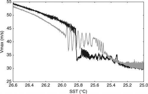
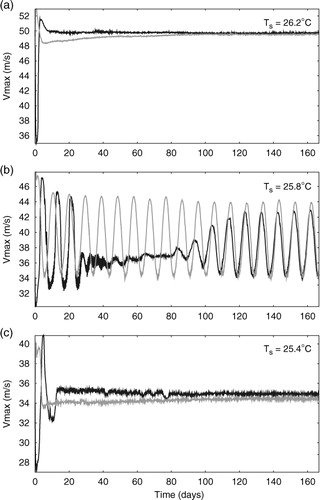
The abrupt jump we find in the cooling experiment, points to the existence of a bistability, whereas the oscillations in the warming experiment rather infer that there is a transition from a fixed-point attractor to a limit cycle indicating a Hopf-bifurcation. To further elucidate the actual behaviour of the dynamical system, we compared experiments started from the cooling and the warming simulations displayed in Fig. 9 at three distinct SSTs in vicinity of the bifurcation point (Fig. 10). For T _s=26.2°C and T _s=25.4°C, the two curves converge, giving further evidence for the existence of a fixed-point attractor (Fig. 10a, c). As can be seen in Fig. 10b, the simulation started from the warming experiment (brighter grey line) reveals the existence of a limit cycle attractor at T _s=25.8°C, with V _max oscillating sinusoidal between ~34 m/s and ~44 m/s. The shape of the V _max -curve in the phase diagram obtained in the simulation that was started from the cooling experiment (dark grey line) is more ambivalent. Over the first 25 days at a constant SST, it displays the behaviour of a limit cycle, too. After this time, the oscillation appears to decline, approaching a value of about 37 m/s, before it starts to oscillate again after 80 days of running time. Finally, the oscillation seems to approach the same period and amplitude that we find in the experiment started from the warming simulation. This strongly suggests that there are two Hopf-bifurcations within a relatively narrow SST range (25.4°C<T _s<26.2°C in the standard case I experiment), the first one at which the fixed-point attractor turns into a limit cycle and the second one, where it is vice-versa. Coming up from higher (lower) SST values, the stable equilibrium solution seems to approach the maximum (minimum) value of the limit cycle in vicinity of the respective bifurcation. However, this behaviour seems to be sensitive to the environmental moisture content. In a drier environment, below a certain value for RH _ref , the Hopf-bifurcations probably disappear (see above).

Fig. 10 Time development of maximum horizontal wind speed in case I for fix SST values in the vicinity of the bifurcation from top to bottom: (a) T _s=26.2°C, (b) T _s=25.8°C and (c) T _s=25.4°C. Each simulation was started at the respective SST from the simulation with decreasing SST (dark grey lines) and increasing SST (brighter grey line) in time (cf. Fig. 9).

5. Discussion

In several aspects, the results from the convection-resolving model HURMOD, shown in the previous section, do agree with those gained from a conceptual TC model, which was introduced in a precursory study (Schönemann and Frisius, 2012). On the other hand, there are also qualitative differences in the behaviour of these two models. In the following, we will discuss the principal results from HURMOD with respect to those of the low-order model and address possible reasons for their disagreement in some points.

Above a certain SST threshold, we obtain an equilibrium solution, where a stable TC state is reached. In the moist-neutral case N, where neutrality in the environment is achieved via a temperature adjustment, this SST threshold is unrealistically low, i.e. well below tropical SSTs in both models, and the intensity of the storm displays a rather weak dependence on SST. In this respect, the models behave very similar, but their response to changes in the initial environmental humidity in the moist-neutral configuration appears to be remarkably different from each other. In the conceptual model, TC intensity decreases with decreasing relative humidity in the ambient region. This is directly opposite to what we observe in the moist-neutral case N configuration in response to changes in the tropospheric reference relative humidity in HURMOD. In this context, it is important to point out that there are two relevant relative humidity parameters in the low-order model: RH in the free troposphere of the ambient region and RH in the boundary layer below. The effect of the latter has not been discussed in Schönemann and Frisius (2012), but a subsequent analysis exhibits that the response to these two parameters is in opposite direction (not shown). Hence, there is a qualitative agreement among the two models in the moist-neutral configuration with regard to their sensitivity to relative humidity in the boundary layer of the inflow region. The discrepancy regarding the sensitivity to environmental RH at mid-tropospheric levels is chiefly attributable to the different way in which the neutrality adjustment of both models works and resulting differences in the impact on tropospheric RH distribution, temperature stratification and outflow temperature. The neutrality adjustment in HURMOD results in a steeper vertical temperature gradient and a lower outflow temperature at a lower environmental relative humidity. This is similar in the low-order model when environmental boundary layer RH is varied and free-tropospheric RH is fixed and vice-versa when free-tropospheric RH is varied and boundary layer RH is fixed.

For the remaining part of this section, we focus on the discussion of the non-neutral case I and J. In both models, HURMOD and the conceptual model, the equilibrium solution is independent of the initial vortex strength, as long as it does not undershoot a certain limit, i.e. the strong TC state is represented by a fixed-point attractor. The finite amplitude nature of TCs, referring to the existence of an amplitude threshold with respect to the strength of the initial disturbance, has been discovered in model experiments by Rotunno and Emanuel (1987) and becomes also evident from HURMOD simulations. In HURMOD, the vortex strength limit or amplitude threshold is sensitive to the tropopause temperature and atmospheric moisture content (cf. Fig. 5) and obviously exists over the whole SST range investigated in the study at hand. On the other hand, in the low-order model, the amplitude threshold vanishes beyond a certain SST, so that even tiniest initial disturbances would sooner or later grow into a strong TC [cf. Fig. 14b in Schönemann and Frisius (2012)]. This may be possibly due to the comparatively rudimentary representation of turbulence in the conceptual model, which does not incorporate the effect of horizontal eddy-diffusion. However, for now, this issue remains highly speculative.

As has been depicted in the previous section, there is a second, SST-dependent amplitude threshold, below which, according to the SSHS classification, TCs only reach tropical storm or minor TC strength. Looking at the case I and J configuration, we see that the SST of that amplitude threshold is sensitive to the environmental (reference) lapse rate and tropopause temperature in a qualitatively similar manner as the amplitude threshold defined by a subcritical saddle node bifurcation in the low-order model [cf. Fig. 8 in Schönemann and Frisius (2012) and Figs. 7, 8 above]. However, with view to the fact that major TCs can form from initial wind speeds close to zero beyond a certain SST in the conceptual model, the amplitude threshold there can probably not be identified with the SST-dependent amplitude threshold in HURMOD. Notwithstanding, the sensitivity to the reference lapse rate and the related outflow temperature of both TC intensity and the SST above, from which strong TCs may arise, is rather similar among the two models.

The influence of the environmental moisture content is investigated by application of different time-invariant values for relative humidity in the ambient region in the low-order model and different initial values for the tropospheric relative humidity in HURMOD (see Section 4.2). Although, as noted above, these two quantities cannot be considered as perfect analogons, they serve as a measure for the environmental moisture content in the respective model, and in the following, we will refer to both as RH _ref . In the conceptual model, the equilibrium intensity is only slightly sensitive to RH _ref , i.e. for the standard case I configuration, the maximum wind speed only rises by about 0.5 m/s per 10% rise in RH _ref (not shown). The intensity in the corresponding HURMOD simulations exhibits a higher sensitivity to RH _ref (see Fig. 4a).

With regard to the amplitude threshold, both models are visibly sensitive to the environmental moisture content [cf. Fig. 4a in Schönemann and Frisius (2012)]. In HURMOD this becomes evident by comparison of Fig. 5a and 5b. This gives a further indication that the subcritical saddle node bifurcation, marking the SST threshold above which TCs can grow from disturbances close to zero in the low-order model actually corresponds to the lower amplitude threshold in HURMOD rather than to the upper strong TC threshold. The second, or upper amplitude threshold is apparently not captured by the conceptual model. In the following, we aim to elucidate some of the causes of the differences in the equilibrium structure of the two models in the parameter range, where the cyclonic system reaches at least tropical storm or category ITC strength on the SSHS. For this purpose, we will further look at the behaviour of the TC in vicinity of the Hopf-bifurcations and in the limit cycle stage we observe in HURMOD.

Several assumptions and approximations conducted in the conceptual model were adopted from Emanuel's theory on the potential intensity (E-PI) of TCs. One such assumption is that the eye only plays a passive role, and hence entropy exchange between the eye and eyewall can be disregarded. The appropriateness of this simplification is challenged by Persing and Montgomery (2003), who claim that low-level fluxes of high-entropy air from the eye into the eyewall are highly relevant to the maximum intensity TCs can reach. They conclude that the neglect of these fluxes is the major reason for the underestimation of TCs’ potential intensity by E-PI. In opposition to this, Bryan and Rotunno (2009b) argue that eye–eyewall entropy fluxes at low levels provide at most a small contribution to an enhanced maximum intensity. In the light of these two opposing hypotheses, we want to figure out whether eye–eyewall entropy fluxes are relevant for TC intensity in HURMOD and whether they are essential to the existence of the limit cycle in the model. Equivalent potential temperature, stream lines and radial velocity at lower tropospheric levels in the inner part of the storm are plotted for different stages of the limit cycle in Fig. 11 and for the weaker and stronger steady-state in vicinity of the Hopf-bifurcations in Fig. 12, respectively. At first glance, it seems that high-entropy air, coming from the eye and entering the eyewall, may indeed play a decisive role in stronger TCs. To test this, we carried out two sensitivity experiments in analogy to those performed by Bryan and Rotunno (2009b). For this purpose, the limit cycle simulation shown in Fig. 10b and 11 has been continued for 2000 h with 150% of the value of the surface exchange coefficient for heat and moisture, i.e. C _H =1.8·10⁻³, within (1) a radius of 10 km and (2) a radius of 12 km. The first sensitivity experiment, where the increase in C _H is confined to the eye, does not exhibit considerable changes in the course of the oscillation regarding the storm structure and its maximum intensity outside the eye. On the other hand, in the second sensitivity experiment, where the region of increased surface enthalpy fluxes is slightly extended reaching into the inner eyewall, the amplitude of the oscillation rises and a maximum wind speed of up to ~46 m/s instead of 44 m/s is reached at the maximum stage of the limit cycle (not shown). So, while enhanced entropy fluxes beneath the innermost part of the eyewall do result in a distinctly increased intensity, we find that low-level entropy fluxes from the eye into the eyewall do not seem to be relevant to the PI of TCs, which agrees with results of Bryan and Rotunno (2009b). In this regard, the assumption that the eye itself responds to its surroundings rather than it actively acts on it, seems to be fairly reasonable.

Fig. 11 Equivalent potential temperature θ _e (colour shadings), stream lines (white) and radial velocity (contour lines) at lower tropospheric levels for the inner part of the TC in the case I standard configuration at different phases of the limit cycle from top to bottom: (a) maximal intensity at maximum, (b) declining intensity, (c) minimal intensity and (d) increasing intensity. Higher θ _e -values are displayed in reddish shades, lower θ _e -values in bluish shades. Inward flow is indicated by dashed lines, zero-radial velocity by thick grey line and outward flow by solid black lines. The contour interval is 1 m/s. The location of V _max is marked by a black circle.

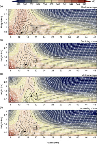
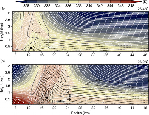
Fig. 12 As in Fig. 11, but for the respective stable states surrounding the limit cycle: (a) at T _s=25.4°C and (b) T _s=26.2°C.

In a follow-up study, Bryan and Rotunno (2009a) argue that gradient–wind imbalance, and associated supergradient winds, is the determining factor to explain the exceedance of the maximum TC intensity predicted by E-PI (also referred to as ‘superintensity’). Concerns about the applicability of the so-called balanced-vortex assumption in the context of TCs have been raised already many decades ago (e.g. Gray (1962), Ooyama (1969) and citations herein). The difference between tangential wind and gradient wind, v–v _gr , as well as vertical wind velocity in the eyewall region, are plotted for different stages of the limit cycle in Fig. 13 and for the weaker and stronger steady-state in vicinity of the Hopf-bifurcations in Fig. 14, respectively. Here, it can be seen that strong upward motion in the boundary layer coincides with enhanced supergradient winds. Moreover, the stronger is the TC, the higher are supergradient winds, and the more dominant is the primary maximum in upward motion from lower tropospheric levels. At the lower stable state (Fig. 14a), the intensity of the secondary (outer) vertical wind maximum relative to that of the primary (inner) maximum is considerably higher than at the upper stable state (Fig. 14b). This behaviour is also reflected in a certain back-and-forth shift of the upward motion between the inner- and outer eyewall that feeds the deep convection, as can be seen by comparison of the different stages of the limit cycle (Figs. 11 and 13). Considering the evolution of the maximum supergradient wind under uniform surface cooling (Fig. 15) in comparison to that of maximum tangential wind (Figs. 7 and 8) provides further evidence on a link between intensity and superintensity. Beside that maximum supergradient winds decrease with v _max in stronger TCs, the onset of considerably enhanced fluctuations and a stronger trend in the decline of (v–v _gr ) _max coincide with the bifurcation that forms the upper strong TC threshold. Hence, the assumption of gradient–wind balance applied in the low-order model may be a possible reason why Hopf-bifurcations as observed in HURMOD are not captured by the conceptual model.

Fig. 13 Difference between tangential wind and gradient wind (colour shadings), and vertical velocity (contour lines) for the inner part of the TC in the case I standard configuration at different phases of the limit cycle from top to bottom: (a) maximal vortex strength, (b) declining strength, (c) minimal strength and (d) increasing strength. Red shades indicate supergradient winds, blue shades indicate subgradient winds, and white areas are in or close to gradient wind balance. Downward flow is indicated by dashed lines and upward flow by solid lines. The contour interval is 0.6 m/s. The location of V _max is marked by a black circle.

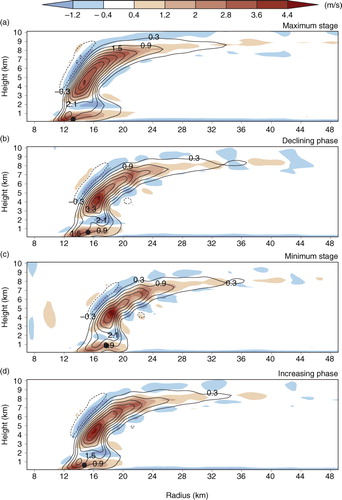
Fig. 14 As in Fig. 13, but for the respective stable states surrounding the limit cycle: (a) at T _s=25.4°C and (b) T _s=26.2°C. Note: The colour scale interval is larger than in Fig. 13.

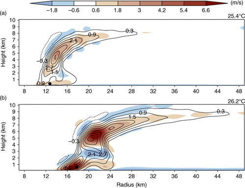
Fig. 15 Development of maximum supergradient wind, (v–v _gr ) _max , with decreasing SST with time at a cooling rate of 10⁻³°C/hin the standard configuration of case J (grey solid line), and case I with differing parameter values: RH _ref =70% and T _s=−70°C (green solid line), RH _ref =50% and T _s=−70°C (orange dotted line), and RH _ref =70% and T _t =−60°C (purple dashed line). Average values over the last 120 h of the 4000 h-runs at fixed SSTs are plotted with different markers for case J (diamonds), case I with RH _ref =70% and T _t =−70°C (circles), RH _ref =50% and T _t =−70°C (squares), and RH _ref =70% and T _t =−60°C (triangles). Error bars display the full range of maximum supergradient wind during the last 120 h of the long-term runs.

Another possible cause for the differences in the bifurcation structure of the two models, may lie in the low-order model assumption that the potential radius of maximum winds (PRMW), given by with v=V _max and r=RMW, is an exogenous parameter, which is constant and independent of environmental conditions. As a consequence, the stronger is the mature TC in the conceptual model, the smaller is its final RMW. In contrast, in the convective model, the RMW appears to depend on the intensity of the storm in the opposite way: the higher the maximum wind speed in the mature TC stage, the larger the vertical and radial extent (referring to both the RMW and the radius of the inflow layer) of the TC. The decreasing trend of the RMW with decreasing V _max is clearly visible in Fig. 16, where the steady-state RMW is plotted against V _max for case J at different SSTs, and several different configurations with respect to the choice of RH _ref , T _s and T _t for case I. Different symbols are used to depict the relation between V _max and the RMW under variation of each one of these three parameters with the two remaining parameters having a fix value. Thereby, it becomes apparent that the relation between the RMW and V _max in HURMOD depends on the environmental moisture content, surface temperature and temperature stratification. For example, it can be seen that the RMW is more sensitive to changes in intensity induced by variation of T _s in a drier environment than in a rather moist environment. The sensitivity of the relation between V _max and the RMW to the choice of environmental parameters implies that the PRMW also depends on this choice. Indeed, the sensitivity behaviour of the PRMW is qualitatively very similar to that of the RMW as becomes evident by comparison of Figs. 16 and 17. 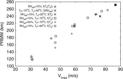In the latter, the steady-state PRMW is plotted against V _max , and it can be seen that for 30 m/s≤V _max <90 m/s the PRMW value ranges from ~115 km to ~275 km. These results show that assuming the PRMW to be an independent constant parameter is very rough and infer that a prescription of the PRMW as a function of the initial environmental conditions would be more appropriate. However, to develop a refined parameterisation of the PRMW within the low-order model, the nature of such a relation needs further investigation, which is beyond the scope of this work.

Fig. 16 Radius of maximum wind speed (km) versus maximum horizontal wind speed (m/s) from average values over the last 120 h of the 4000 h-runs at different values for T _s and T _t =f(T _s) in case J (diamonds), and case I with T _t =−70°C and T _t =30°C for different values in RH _ref (crosses), RH _ref =70% and T _s=30°C for different values in T _t (triangles), RH _ref =70% and T _t =−70°C for different values in T _s (squares), RH _ref =50% and T _t =−70°C for different values in T _s (plus signs), and RH _ref =70% and T _t =−60°C for different values in T _s (circles). Note: identical results in this plot stem from the same model experiment.

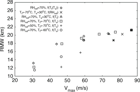
Fig. 17 As in Fig. 16, but with the potential radius of maximum wind speed on the ordinate.

6. Summary and conclusions

For the purpose of investigating the equilibrium and bifurcation structure of TCs in a model of intermediate complexity, we carried out long-term model experiments with the axisymmetric convection-resolving model HURMOD. The results reveal that the mature stage of a strong TC within the model has the character of a fixed-point attractor, where the final state is independent of the initial size and strength of the disturbance above a certain threshold. This is in qualitative agreement with the results of a low-order model introduced by Schönemann and Frisius (2012), whose simplicity allowed to determine equilibria by means of an eigenvalue analysis.

TC intensity and the critical initial vortex strength necessary for TC formation are sensitive to tropospheric humidity and temperature lapse rate. The steeper the lapse rate and the more humid the air, the lower is the amplitude threshold to cyclogenesis and the higher is its PI. A larger difference between the SST and outflow temperature of TCs implies a higher thermodynamic efficiency resulting in an enhanced intensity and a reduced static stability facilitates convection (Wada et al., 2012). Further hints to the fact that not merely SST is relevant to TC activity are given in a recent study by Emanuel et al. (2013). Their analysis of observational and reanalysis data shows that changes in TC activity over the North Atlantic are highly correlated to temperature changes in the upper troposphere. The sensitivity to temperature stratification in HURMOD is also in accordance with the observed non-local response of TC intensity over the North Atlantic found by Swanson (2008). Regarding intensity, HURMOD's results suggest that the temperature stratification plays a more important role than environmental relative humidity. On the other hand, environmental relative humidity appears to be highly relevant to the frequency of occurrence of TCs, which agrees with results from previous modelling and observational studies (Gray, 1979; Zhao and Held, 2012).

Tropical cyclone dynamics in HURMOD in response to changes in the SST is characterised by a Hopf-bifurcation, where a fixed-point attractor turns into a limit cycle attractor, and a second Hopf-bifurcation at a slightly lower SST, where the limit cycle attractor turns into a fixed-point attractor, before the system becomes chaotic and finally unstable at lower SSTs. The SST range within which the bifurcations are observed is strongly sensitive to the tropospheric lapse rate. Moreover, the existence of the Hopf-bifurcations is also found to depend on the environmental moisture content. In a drier environment, they seem to disappear. Presuming a moist-neutral environment (case N), HURMOD does not exhibit any bifurcations within the range of tropical SSTs. Furthermore, in case N the intensity is found to be enhanced in a drier environment, rather than the other way round, which would be more realistic. Therefore, we conclude that the moist-neutral assumption in case N results in a rather unrealistic behaviour of the modelled TC, compared to that in the non-neutral case I and J.

Apart from the generally higher susceptibility to the occurrence of small-scale fluctuations in HURMOD, no Hopf-bifurcations occur in the low-order model introduced in a previous study (Schönemann and Frisius, 2012), and in contrast to HURMOD, strong TCs can develop from very small disturbances close to the state of rest, given that the environmental moisture and temperature conditions are sufficiently favourable. At this point, we can indicate two principal differences in the conception of the low-order model and HURMOD, which may be chiefly responsible for these structural differences among the two models: In the conceptual model, (1) the assumption that the vortex is in gradient–wind balance is made and (2) the PRMW is considered as constant and independent of initial conditions. In contrast, in HURMOD, considerable supergradient winds arise in TC strength storms, which agrees with the findings by Bryan and Rotunno (2009b). Furthermore, the comparison of steady-state results from different model configurations reveals that the PRMW displays a decreasing tendency with decreasing maximum intensity in HURMOD. The tendency itself appears to be sensitive to the initial tropospheric temperature and moisture conditions. Consequently, we expect that the consideration of a parameterisation for the PRMW as a function of the thermodynamic reference state in the low-order model would result in a better agreement among the two models of different complexity. The last point may be subject to a future study.

Overall, the results from HURMOD presented herein, as well as the results from the low-order model, infer that the value of the SST threshold, above which strong TCs may occur, rises to higher values with increasing tropopause temperature; decreasing temperature lapse rate; and decreasing environmental moisture content. These findings indicate that the observed SST threshold for cyclogenesis depends on the climate state and thus can be expected to shift in response to global and regional climate change. Beside the question on possible extensions of the low-order model with the aim to achieve a better agreement with the high-resolution model, an evaluation of the validity of this climate state dependence and other tendencies found in this study in a more sophisticated 3-D model or a global circulation model may provide some material for further investigations.

Acknowledgements

This work was supported by the DFG within the Cluster of Excellence 177 Integrated Climate System Analysis and Prediction (CliSAP). The authors would also like to thank two anonymous reviewers for their constructive criticism on this work.

Notes

¹Emanuel, K. A. and D. S. Nolan, 2004: Tropical Cyclone Activity and the Global Climate System. The 26th Conference on Hurricanes and Tropical Meteorology.

²For reasons of simplicity, we only work with ‘warm-rain’ simulations in the present work, i.e. the ice phase is not considered in the calculation of the water budget, and the cloud–micro-physical parameterisation follows a Kessler type scheme. For possible effects of the inclusion of an ice phase in axisymmetric models, we may refer the reader to previous studies by Willoughby et al. (1984) as well as Frisius and Hasselbeck (2009).

³Note, in the low-order model, moist neutrality is either maintained by an adjustment of the boundary layer relative humidity or by a lapse rate adjustment, whereas a physically more consistent combination of both a moisture and a temperature profile adjustment, cannot be realised in the low-order model. Therefore, case N is subdivided into case N1 and N2 in the low-order model.

⁴The decay rate is chosen to be very slow in order to stay close to the respective equilibrium, which eases the detection of bifurcations.

⁵To test the robustness of the limit cycle behaviour, the simulations at 25.8°C were continued and run 2000 hours longer (not shown). The oscillation with a period of about 225 hours is sustained in both experiments.

⁶We note that this question cannot be answered with certainty here, since we have not tested whether spontaneous cyclogenesis occurs at SSTs much higher than 30°C in HURMOD or not.

References

- Bister M , Emanuel K. A . Dissipative heating and hurricane intensity. Meteorol. Atmos. Phys. 1998; 65: 233–240.
- Black A. K , Ásaro E. A. D , Drennan W. M , French J. R , Niiler P. P , co-authors . Air–sea exchange in hurricanes. Synthesis of observations from the coupled boundary layer air–sea transfer experiment. Bull. Am. Meteorol. Soc. 2007; 88: 357–374.
- Blackadar A. K . The vertical distribution of wind and turbulent exchange in a neutral atmosphere. J. Geophys. Res. 1962; 67: 3095–3102.
- Bryan G. H , Fritsch J. M . A benchmark simulation for moist nonhydrostatic numerical models. Mon. Weather Rev. 2002; 130: 2917–2928.
- Bryan G. H , Rotunno R . Evaluation of an analytical model for the maximum intensity of tropical cyclones. J. Atmos. Sci. 2009a; 66: 3042–3060.
- Bryan G. H , Rotunno R . The influence of near-surface, high-entropy air in hurricane eyes on maximum hurricane intensity. J. Atmos. Sci. 2009b; 66: 148–158.
- Bryan G. H , Rotunno R . The maximum intensity of tropical cyclones in axisymmetric numerical model simulations. Mon. Weather Rev. 2009c; 137: 1770–1789.
- Camargo S. J , Ting M , Kushnir Y . Influence of local and remote SST on North Atlantic tropical cyclone potential intensity. Clim. Dynam. 2013; 40: 1515–1529.
- Camp J. P , Montgomery M. T . Hurricane maximum intensity: past and present. J. Atmos. Sci. 2001; 129: 1704–1717.
- Emanuel K. A . An air–sea interaction theory for tropical cyclones. Part I: steady-state maintenance. J. Atmos. Sci. 1986; 43: 585–604.
- Emanuel K. A . The finite-amplitude nature of tropical cyclogenesis. J. Atmos. Sci. 1989; 46: 3431–3456.
- Emanuel K. A . Sensitivity of tropical cyclones to surface exchange coefficients and a revised steady-state model incorporating eye dynamics. J. Atmos. Sci. 1995; 52: 3969–3976.
- Emanuel K. A , Solomon S , Folini D , Davies S , Cagnazzo C . Influence of tropical tropopause layer cooling on Atlantic hurricane activity. J. Clim. 2013; 26: 2288–2301.
- Fairall C. W , Bradley E. F , Hare J. E , Grachev A. A , Edson J. B . Bulk parameterization of air–sea fluxes: updates and verification for the COARE algorithm. J. Clim. 2003; 16: 571–591.
- Frisius T , Hasselbeck T . The effect of latent cooling processes in tropical cyclone simulations. Q. J. Roy. Meteorol. Soc. 2009; 135: 1732–1749.
- Frisius T , Wacker U . Das massenkonsistente axialsymmetrische Wolkenmodell HURMOD. Deutscher Wetterdienst, Arbeitsergebnisse. 2007; 85: 42.
- Gray W. M . On the balance of forces and radial accelerations in hurricanes. Q. J. Roy. Meteorol. Soc. 1962; 88: 430–458.
- Gray W. M , Shaw D. B . Hurricanes: their formation, structure and likely role in the tropical circulation. Meteorology over the Tropical Oceans. 1979; Bracknell, Berkshire: Royal Meteorological Society. 155–218.
- Hill K. A , Lackmann G. M . Influence of environmental humidity on tropical cyclone size. Mon. Weather Rev. 2009; 137: 3294–3315.
- Holland G. J . An analytic model of the wind and pressure profiles in hurricanes. Mon. Weather Rev. 1980; 108: 1212–1218.
- Kepert J. D . Slab- and height-resolving models of the tropical cyclone boundary layer. Part I: comparing the simulations. Q. J. Roy. Meteorol. Soc. 2010; 136: 1686–1699.
- Kepert J. D . Choosing a boundary layer parameterization for tropical cyclone modeling. Mon. Weather Rev. 2012; 140: 1427–1445.
- Knaff J. A , DeMaria M , Sampson C. R , Peak J. E , Cummings J , Schubert W. H . Upper oceanic energy response to tropical cyclone passage. J. Clim. 2013; 26: 2631–2650.
- Mei W , Pasquero C . Spatial and temporal characterization of sea surface temperature response to tropical cyclones. J. Clim. 2013; 26: 3745–3765.
- Ooyama K . Numerical simulation of the life cycle of tropical cyclones. J. Atmos. Sci. 1969; 26: 3–40.
- Ooyama K. V . Conceptual evolution of the theory and modelling of the tropical cyclone. J. Meteorol. Soc. Jpn. 1982; 60: 369–379.
- Persing J , Montgomery M. T . Hurricane superintensity. J. Atmos. Sci. 2003; 60: 2349–2371.
- Rotunno R , Emanuel K . An air–sea interaction theory for tropical cyclones. Part II: evolutionary study using a nonhydrostatic axisymmetric numerical model. J. Atmos. Sci. 1987; 44: 542–561.
- Schönemann D , Frisius T . Dynamical system analysis of a low-order tropical cyclone model. Tellus A. 2012; 64: 15817.
- Swanson K. L . Nonlocality of Atlantic tropical cyclone intensities. Geochem. Geophys. Geosyst. 2008; 9: Q04V01.
- Tang B , Emanuel K . Midlevel ventilations constraint on tropical cyclone intensity. J. Atmos. Sci. 2010; 67: 1817–1830.
- Tang B , Emanuel K . Sensitivity of tropical cyclone intensity to ventilation in an axisymmetric model. J. Atmos. Sci. 2012; 69: 2394–2413.
- Wada A , Usui N , Sato . Relationship of maximum tropical cyclone intensity to sea surface temperature and tropical cyclone heat potential in the North Pacific Ocean. J. Geophys. Res. 2012; 117: D11118.
- Wang Y . How do outer spiral rainbands affect tropical cyclone structure and intensity?. J. Atmos. Sci. 2009; 66: 1250–1273.
- Willoughby H. E , Jin H.-L , Lord S. J , Piotrowicz J. M . Hurricane structure and evolution as simulated by an axisymmetric, nonhydrostatic numerical Model. J. Atmos. Sci. 1984; 41: 1169–1186.
- Xu J , Wang Y . Sensitivity of the simulated tropical cyclone inner-core size to the initial vortex size. Mon. Weather Rev. 2010; 128: 4135–4157.
- Yanase W , Satoh M , Taniguchi H , Fujinami H . Seasonal and intraseasonal modulation of tropical cyclogenesis environment over the Bay of Bengal during the extended summer monsoon. J. Clim. 2012; 25: 2914–2930.
- Yu J , Wang Y , Hamilton K . Response of tropical cyclone potential intensity to a global warming scenario in the IPCC AR4 CGCMs. J. Clim. 2010; 23: 13541373.
- Zeng Z , Chen L , Wang Y . An observational study of environmental dynamical control of tropical cyclone intensity in the Atlantic. Mon. Weather Rev. 2008; 136: 3307–3322.
- Zhang J. A , Marks F. D , Montgomery M , Lorsolo S . An estimation of turbulent characteristics in the low-level region of intense hurricanes Allen (1980) and Hugo (1989). Mon Weather Rev. 2011; 139: 1447–1462.
- Zhang J. A , Montgomery M . Observational estimates of the horizontal eddy diffusivity and mixing length in the low-level region of intense hurricanes. J. Atmos. Sci. 2012; 69: 1306–1316.
- Zhao M , Held I. M . TC-permitting GCM simulations of hurricane frequency response to sea surface temperature anomalies projected for the late-twenty-first century. J. Clim. 2012; 25: 2995–3009.
- Zhao M , Held I. M , Lin S.-J , Vecchi G. A . Simulations of global hurricane climatology, interannual variability, and response to global warming using a 50-km resolution GCM. J. Clim. 2009; 22: 6653–6678.