Contribution to the global air–sea CO₂ exchange budget from asymmetric bubble-mediated gas transfer

ABSTRACT

Quantifying air–sea gas exchange is an essential element for predicting climate change due to human activities. Air–sea gas exchanges take place through both the sea surface and bubbles formed during wave breakings. Bubble-mediated gas transfers are particularly important at high wind regions. Bubble-mediated gas transfers are separated into symmetric and asymmetric transfers. Their transfer fluxes are respectively proportional to the gas concentration difference between the atmosphere and ocean surface water, and to the atmospheric gas concentration alone. To quantify the role of asymmetric transfers in the global carbon dioxide (CO₂) transfer budget, a parameterisation scheme of asymmetric transfer is developed, which is constrained by gas equilibrium supersaturation in the ocean surface. By establishing a bound for the global mean gas equilibrium supersaturation in ocean surface water, we found that the global ocean uptake by bubble-mediated asymmetric gas transfer is a substantial part of the total air–sea CO₂ uptake budget (over 20%). It is found that, over the past half century, the global asymmetric ocean CO₂ uptake has increased about a total of 40% on a steadily trend, as a consequence of the increasing atmospheric CO₂ concentrations.

• air-sea gas exchanges
• bubbles
• oceanic CO₂ uptakes
• equilibrium saturations
• breaking waves

1. Introduction

The ongoing build-up of carbon dioxide (CO₂) in the atmosphere due to anthropogenic CO₂ emissions is affecting the environment on both local and global scales. The total present-day anthropogenic emissions of CO₂ to the atmosphere have reached a level about 7 Pg C yr⁻¹ (see Marland, G., Boden, T. A., Andres, R. J. Global, regional, and national fossil-fuel CO₂ emissions http://cdiac.ornl.gov/trends/emis/overview.html 2006). A little less than half of the emitted CO₂ gas is accumulated in the atmosphere, the remainder is either dissolved in the ocean or taken up by terrestrial ecosystems. While previous studies have consistently demonstrated that the ocean is a sink for atmospheric CO₂, the estimated uptake values are highly divergent (Keeling et al., 1996; Prentice, 2001; Sarmiento and Gruber, 2002; Takahashi et al., 2002; Sabine at al., 2004). Oceanic CO₂ uptake makes the ocean surface increasingly more acidic, which is likely to have serious consequences for ocean ecology (Caldeira and Wickett, 2003; Feely et al., 2004; Orr et al., 2005).

The air–sea CO₂ flux, F, can be directly estimated via the following bulk formula:1

where k is the gas-transfer velocity, α is gas solubility, and ΔpCO₂ is the difference in partial pressure of the gas across the diffusive layer of the sea surface. Part of the uncertainty involved in direct calculations of air–sea gas fluxes using eq. (1) stems from the parameterisation of transfer velocity (Wanninkhof et al., 2009). Most parameterisation models occur in the form of simple functions of wind speed with empirically determined parameters, including the piecewise linear form (Liss and Merlivat, 1983), quadratic forms (Wanninkhof, 1992; Nightingale et al., 2000; Ho et al., 2006), cubic forms (Wanninkhof and McGillis, 1999; McGillis et al., 2001 2004; Monahan, 2002), and hybrid forms which differentiate transfers through sea surface and bubbles (Monahan and Spillane, 1984; Asher and Wanninkhof, 1998; Woolf, 2005). The transfer velocity obtained from these models for a given wind speed varies by a factor of at least 2. To reduce uncertainty in global uptake calculations, constraints such as the global bomb-¹⁴C oceanic uptake are used to determine the parameterisation coefficients. The oceanic uptake estimation based on such transfer velocity parameterisations shows minor interannual variability as compared with changes in atmospheric CO₂ (Lee et al., 1998). Recent developments in transfer velocity parameterisation consider not only wind speed but also other environmental variables, such as heat fluxes and wave conditions (Soloviev and Schlüssel, 1994; Fairall et al., 2000; McNeil and D'Asaro, 2007; Woolf et al., 2007).

The aim of the present study is to examine the percentagewise contribution to the global budget of CO₂ air–sea flux from asymmetric bubble-mediated gas transfer that can easily be overlooked when calculating ocean CO₂ uptakes using eq. (1), by accounting for only symmetric gas transfers. Here, the symmetric and asymmetric gas transfers refer to the transfers that is proportional to the partial pressure difference across the diffusive layer of the sea surface (e.g. eq. (1)) and that is proportional to atmospheric gas partial pressure, respectively.

Air–sea gas exchanges take place through air–sea interface and through bubbles. Breaking waves are the major source of ocean surface bubbles. The gas partial pressures inside ocean surface bubbles is generally higher than the partial pressures of the same gases in the atmosphere. This is because hydrostatic pressure and surface curvature contribute significant extra pressure inside the gas bubbles. Gas transfer mediated by bubbles is more efficient than the transfer through the air–sea interface. The bubble-mediated transfer is not zero even when the partial pressure difference across the diffusive layer of the sea surface is zero. The extra pressure of hydrostatic and surface tension results in a slight supersaturation of dissolved gases in sea surface waters worldwide. Craig and Weiss (1971) first suggested that bubble mediated transfer can be separated into two parts: a major symmetric component and a minor asymmetric component.

In the next section, we will briefly explain the unfamiliar subject of bubble-mediated asymmetric gas transfer and the underlying physical processes. Based on the dynamical analysis, a parameterisation scheme for bubble-mediated asymmetric gas transfer is then postulated. The bound for the parameterisation constant established in Section 3 is based on combined laboratory and oceanic observations, especially the estimation from climatological O₂ surface saturations. By applying this parameterisation, the global CO₂ air–sea exchange budget via bubble-mediated asymmetric gas transfer is computed. The data and numerical methods are detailed in Section 4. The global characteristics of bubble-mediated asymmetric gas transfer are given accordingly in Section 5.

2. Parameterisation of bubble-mediated asymmetric transfer

2.1. Asymmetric transfer

The above bulk flux eq. (1) is a practical approximation of the Fickian flux equation:2

The thermodynamic potential, ΔC, is the difference in effective gas concentration across the waterside diffusive layer, because the gas transfer is retarded within the diffusive boundary layer on the waterside for weakly soluble gases (e.g. CO₂). The flux can be further separated into the contribution from direct transfer though air–sea interface and the sum of contributions from all bubbles over their bubble life time injected from the same unit of sea surface:3

where the subscripts s and b represent the sea surface and bubbles, respectively. S(i) and L(i) are the surface area and trajectory of an individual bubble. j(i) is the individual bubble gas transfer velocity, and is the difference in dissolved gas concentration around the corresponding bubble. Bubbles generated by wave breaking are believed to rapidly attain a spatial distribution of dynamic equilibrium after a short transition period following their formation. Merlivat and Memery (1983) proposed that the bubble-mediated flux of a gas, F _b , in a dynamic equilibrium regime can be modelled as the sum of individual bubble transfers during their lifetimes in the water, , weighted by the bubble source distribution, :4

where r _i and z _i are the initial size and depth of bubbles, respectively. Bubble source distribution function prescribes the number of bubbles per unit radius which are initially submersed to the initial depth per unit of time. The amount of gas transfer by each bubble depends not only on its initial size and depth in the water, but also on its travel path and the amount of time the bubble remained in the water. Here, is the mean gas transfer of a bubble at an initial depth of z _i with size of r _i averaged over varies bubble trajectories.

Very small bubbles (<0.005 cm) that are injected into deep water can be totally dissolved in water resulting a net transfer of gases of atmospheric composition into water. Let be the air-volume-injection rate for all these small bubbles. The corresponding (injection type of) gas flux, , is the injection rate of total molar content:5

where R is ideal gas constant, and T is the temperature of the bubbles. This transfer component is asymmetric because it is proportional to the gas concentration in equilibrium with the atmosphere above, C _a . The corresponding injection transfer velocity, , is therefore:6

For large bubbles, gas exchange continues until bubbles reach the water surface. , where n _i and n _f are the molar contents of tracer gases contained in the bubble at initial and final stages, and denotes for the ensemble average. The equation of molar contents of tracer gas, n, for a spherical bubble, is (see Appendix S1 for derivation):7

where r is the bubble radius, and p _w is the partial pressure of tracer gas of surrounding water. V is the volume of the bubble. is Ostwald solubility coefficient. D and ν are the gas molecular diffusivity in sea water and the kinematic viscosity of sea water, respectively. Individual bubble gas transfer velocity j is proportional to D ^d ν ^1/2-d where the exponent constant, d, varies from 1/2 to 2/3 depending on the Reynolds number. The scaled bubble transfer velocity j*=j(D ^d ν ^1/2–d )⁻¹ is independent of gas physical properties. The volume of the bubble varies with water depth due to hydrostatic compression and the amount of gases exchanged with water, i.e. , where n ⁱ is the different gas constitution of the bubble. depends mainly on the major atmospheric gases of N₂ and O₂. Large bubbles (>0.03 cm) rise faster than the appreciable changes in fractional molar content due to small solubilities of the major gases of O₂ and N₂, therefore, the corresponding dissolution volume change can be discarded as a first order approximation. In addition, the background vertical motions of coherent flows, such as Langmuir cells, are in general much smaller than the large bubble terminal speed. Under these approximations, the equation of molar content of tracer gases becomes linear and its solution can be found in a form of (Appendix S1):8

Thus, gas transfer flux by large bubbles, which is often referred to as exchange type transfer, can be approximated in the form of:9

where:10

can be further extended to also include small bubbles of injection type transfer. Bubble-mediated gas flux in the form of eq. (9) has been suggested based on some simple physical arguments (Craig and Weiss, 1971; Fuchs et al., 1987) and backed by a number of previous simulation-based studies (Memery and Merlivat, 1985; Woolf and Thorpe, 1991; Keeling, 1993). Here, we provide the first analytic proof for this approximation. An equivalent formulation of bubble transfer of eq. (9) is in terms of ingassing (pure invasion) and outgassing (pure evasion) transfer velocities, k _in and k _out (see Keeling, 1993):11

where C _w is the gas concentration of sea water that surrounds bubbles. Ingassing transfer depends on the gas concentration in the air over the water, while outgassing transfer depends on the gas concentration of sea surface water. When gas transfer velocities of ingassing and outgassing are equal, the transfer is symmetric. Asymmetric bubble transfer velocity, , is the difference between the one-way bubble exchange velocities of ingassing and outgassing, . The asymmetric nature of gas transfer mediated by bubbles is caused by over pressure within bubbles and gas dissolution.

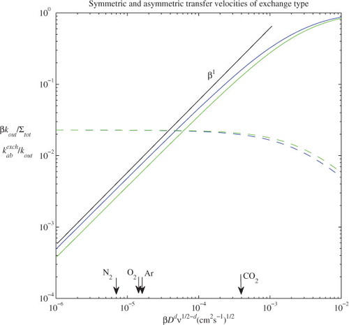
An example of and as a function of gas chemo-physical parameter, θ=βD ^d ν ^1/2−d , is shown in Fig. 1. This is an extended calculation from the early work by Keeling (1993). Our calculation allows the bubble hydrostatic expansion in solving the molar content formula of eq. (7). Bubble radius was kept constant in the early calculations. The volume dissolution reduces the volume slightly, therefore, the more realistic solution should be located between the results of constant bubble size of Keeling (1993) and hydrostatic expansion solutions here. Two bubble spectra are used: (1) Monahan and Zeitilow (1969) with a cut-off at 0.4 cm; and (2) recent work by Deane and Stokes (2002) with a transition at 0.1 cm. As with Keeling (1993), an e-folding depth distribution with a uniform characteristic depth of 25 cm for all bubble sizes is selected. Our calculation shows that: (1) both K _out and are not very sensitive to gas solubility up to the solubility range of gas CO₂, while in the case of fixed bubble size (Keeling, 1993); and (2) the ratio, , is quite constant over this gas solubility range, which is consistent with the Keeling's results (1993). This supports parameterisation schemes of which the proportionality between and is independent of the gas chemo-physical parameter.

Fig. 1.  Exchange type of bubble-mediated transfer velocities as a function of the chemo-physical parameter of gases. The blue curves are calculated based on the bubble spectrum of Deane and Stokes (2002) with a transition at 0.1 cm, and green curves are derived from the spectrum of Monahan and Zeitilow (1969) with a cut off at 0.4 cm. The solid curves are bubble symmetric transfer velocities, k _out, multiplied by the Ostwald solubility coefficient, β, and divided by the rate of total bubble volume, Σ_tot. The dashed curves are the ratio of the asymmetric velocity, , over . The straight black line denotes the slope for a linear function of β. The corresponding chemo-physical parameter values of θ for atmospheric gases CO₂, O₂, Ar and N₂ are marked with arrows. The constant d used for calculating θ is 2/3.

The asymmetric transfer velocity of intermediate sized bubbles, that are not completely collapsed and are close to a solubility-equilibrium with the surrounding water, has a similar form as very small absorbed bubbles but is proportional to the net volume change of the bubble lifetime rather than total volume of bubbles. Therefore, one can allow the air injection velocity to account for not just small bubbles which are fully injected, but also for somewhat larger bubbles which are partially injected. For gases which are not near the concentration equilibrium, the air injection process can generally be neglected because, in these cases, the net volume change of the partially injected bubbles is controlled by dissolution of the major gases (weak non-linearity of bubble dynamics). The numerical simulations by Woolf and Thorpe (1991) show that this non-linear effect is small and proportional to the gas saturation levels.

The asymmetric nature of bubble-mediated gas transfer is suggested as one of the causes of worldwide gas supersaturation in ocean surface water (Craig and Weiss, 1971). When atmospheric gas concentration is in transfer equilibrium with ocean surface waters, i.e. the total net gas flux is zero, the fractional surface saturation is equal to . f _e is a measure of the fractional supersaturation of ocean surface water by bubble-mediated gas transfer and depends on both bubble and surface transfer velocities in general. In some bubble transfer parameterisation schemes, the asymmetric transfer is expressed in terms of f _e (Woolf, 1997; McNeil and D'Asaro, 2007; Woolf et al., 2007):12

Woolf and Thorpe (1991) proposed a parameterisation of wind speed square for f _e . When bubble transfer becomes dominant at high wind, surface transfer is relative small. Therefore, the fractional surface saturation approaches to the ratio in the transfer equilibrium state. Woolf (1997) and Woolf et al. (2007) proposed a parameterisation of K _out in a form of:13

Here, , varying with α ⁻¹, is the bubble transfer velocity limit when concentrations of bubbles and the surrounding water are in full equilibrium. is the other limit of bubble transfer velocity when bubbles and the surround water are in non-equilibrium. is the ensemble average of individual bubble transfer velocities and is proportional to D ^−d ν ^d−1/2. The non-dimensional parameter of exponent, f, is related to the breadth of bubble distribution.

The transfer flux ratio of asymmetric transfer to symmetric transfer is proportional to both f _e and C _a /ΔC _s . The asymmetric oceanic CO₂ uptake increases in direct proportion to the increases in atmospheric CO₂ concentration, as the ocean surface CO₂ maintains a dynamically stable equilibrium-balance with atmospheric CO₂ (i.e. ΔC _s is approximately constant at longer than yearly scales (Takahashi et al., 2002)). Therefore, the ratio will increase with atmospheric CO₂ concentration. To estimate the ocean CO₂ uptake through asymmetric transfer, a parameterisation constrained by the global mean gas supersaturation is proposed next.

2.2. A parameterisation for the asymmetric transfer

Bubble formation processes of breaking waves are poorly understood. Observations tend to suggest that: (1) there appears to exist universal power laws for the size spectrum and vertical distributions of bubbles (Monahan and Zeitlow, 1969; Kolovayev, 1976; Cipriano and Blanchard, 1981; Koga, 1982; Crawford and Farmer, 1987; Hwang et al., 1990; Deane and Stokes, 2002); and (2) the rate of sea-surface coverage of whitecaps from breaking waves varies approximately with a cubic or higher powers of wind speed, u (Monahan and O'Muircheartaigh, 1980; Erickson et al., 1986; Monahan and Torgersen, 1990; Lamarre and Melville, 1991; Asher et al., 2002). These observational conclusions on bubble distributions infer that the bubble source function, , is proportional to the horizontal surface distribution because the vertical and size distributions of bubbles are all universal. Since the horizontal scale of surface bubble clouds from breaking waves can be represented by the scale of surface whitecaps, the total volume fraction of air injected by breaking waves should be proportional to the rate of sea-surface coverage of whitecaps, W(u), which can be approximated by an empirical function of wind speed u. By this approximation, can be factorised into . is the vertical and size distribution of bubbles which is assumed to have a universal function form. For the convenience of following discussions, we introduce a new set of transfer velocities:14

In general, expressions for N's or B's can be very complicated. There is also a large uncertainty in modelling due to the limitations of our knowledge of wave breaking and subsequent bubble formation processes. However, we can argue that and are largely unaffected by wind speed, as large bubbles rise rapidly compared to the averaged vertical speed of surface-wave orbital motions and convective motions that include Langmuir cells, and turbulent motions. The initial distribution of bubbles with depth depends on the mechanisms of waves breaking and bubble formation, both of which are very complex subjects. Wave intrinsic instabilities and turbulent shear flow structures are the main mechanisms of wave breaking (Melville, 1996). The surface shapes and flow structures of breaking waves should be mainly scaled by these wave instability parameters, and may not be strongly affected by wind directly. Therefore, it is assumed here that is independent of wind as a first order approximation. However, the dominant wave period of sea is a function of wind speed and fetch. This scaling factor of breaking waves is in part already implied, as we argue, in the fractional whitecap coverage factor, W(u).

In our calculations of global CO₂ uptake by asymmetric bubble-mediated gas transfer, and are independent of wind speed as a consequence of the above assumption that is independent of wind. Instead of solving the integral eq. (14) under complicated oceanic conditions, a parameterisation constant, , is introduced with a value constrained by the global climatological mean of the CO₂ equilibrium supersaturation due to bubble-mediated gas transfer, , noted as:15

Where is the mean equilibrium supersaturation averaging over global ocean area, :16

where denotes for climatological mean. In this way, the uncertainties in determining can be bound by our knowledge from observations of the global gas supersaturations due to bubble-mediated gas transfer.

3. Bounds for bubble-mediated equilibrium supersaturation of CO₂

The global average CO₂ supersaturation,, is proposed for constraining the parameterisation constant, The equilibrium supersaturation due to bubble-mediated gas transfer of CO₂ should typically be about 0.1% (Keeling, 1993; Woolf, 1997). Because the oceanic excursions of CO₂ from saturation are unusually large (often greater than 10%), it is difficult to directly access the bubble-mediated equilibrium supersaturation of CO₂ from field surface measurements. These large excursions are dominated by other factors such as upwelling or biological pumping (Takahashi et al., 2002). Nevertheless, the bounds for bubble-mediated equilibrium supersaturation of CO₂ can be established from measurements of other gases through the scaling arguments.

3.1. Scaling of transfer velocity

Unlike surface gas transfers, bubble-mediated gas transfer velocities are also scaled with gas solubility. Gas solubility regulates the equilibrium time of the gas–liquid concentration relative to the pressure change in a bubble, with smaller values of equilibrium time for gases with higher solubility. Most existing parameterisation schemes for bubble-mediated transfer velocity assume a scaling form in powers of Schmidt number and solubility, , as listed in Table 1.

Table 1. Scaling parameters for bubble-mediated transfer velocity ()

	y	z
Jenkins (1988)	2/3	0
Keeling (1993)	0.35	−0.3
Asher et al. (1996)	0.18^a or 0.20^b	−0.37^a or −0.17^b
Schudlich and Emerson (1996) and Hamme and Emerson 2002	1/2	0
Woolf et al. (2007)	0^c ~ 1/2^a,d	−1^c ~ 0^d

^aClean bubbles.

^bDirty bubbles.

^cIn the large solubility limit.

^dIn the small solubility limit.

Many parameterisation models (non-hybrid) of symmetric transfer do not explicitly distinguish scaling differences of direct surface transfer, k _s , and bubble-mediated symmetric transfer, k _out. The scaling for combined k _s and k _out is often assumed to be a uniform Schmidt number scaling (Sc)^−x , where constant x is the Schmidt number dependence, e.g. 2/3 for smooth surfaces or 1/2 for rough surfaces. The Schmidt number scaling is mostly based on laboratory tank experiments which may significantly miss energetic breaking waves (Jähne et al., 1987). When surface transfer dominates over bubble-mediated transfer, such practices are adequate and convenient because k _s +k _out does not strongly depend on solubility. For the hybrid parameterisation models that differentiate contributions from surface and bubble transfers, the scaling formulation of (Sc)^−x only applies to the surface transfer component, k _s .

The injection and exchange parts of asymmetric transfer velocity, and are all parameterised to be proportional to the fractional whitecap coverage therefore, their ratio is not dependent on wind speed in the approximation here. However, since and are scaled differently by solubility and Schmidt number, the ratios vary among gases of different diffusivity and solubility. The exchange component can be scaled roughly the same way as as found by most calculations (Keeling, 1993 and Section 2), and the injection component is scaled inversely with solubility as a result of the proportionality to the atmospheric air constitution. The corresponding injection and exchange parts of equilibrium saturation, and , have different and somewhat complex dependencies on solubility and diffusivity. For two limiting cases of: (a) ; and (b) , we have:

.

From a number of field data sets, it has been estimated that and are comparable in size for O₂ with a favourable scaling form that is equivalent of the case (b) (Hamme and Emerson, 2002 2006). To infer equilibrium saturations of CO₂ from those of O₂ by different scaling parameters, Keeling's model, compared to other models in Table 1, gives the smallest value of ; therefore, it will be used here for a conservative low-bound estimation of equilibrium saturations of CO₂ from that of O₂ and other gases. By Woolf's parameterisation, the bubble transfer velocity, k _out, of O₂ is about twice the transfer velocity of CO₂, which is equivalent to in this particular solubility range.

3.2. Laboratory bubble plume measurements

A laboratory experiment conducted by Asher et al. (1996) on gas exchange by bubble plumes may shed some light on the degree of ocean surface water gas saturation due to bubble-mediated gas transfer. In this experiment, bubbles were formed by injecting water into surface water by a tipping bucket 30 cm above the surface. Their measurements include the fractional area of bubble plume coverage and the bubble-mediated transfer velocities for evasion and invasion of various gases. Their results show that the transfer velocities of invasion and evasion can be fitted nicely onto a linear function of fractional area of bubble plume coverage and a universal dependency of bubble-mediated transfer velocities on gas solubility. On the other hand, k _ab (equal to the difference between invasion and evasion transfer velocities) for CO₂ is too small to be resolved from their data, which was limited by their measurement accuracy. Measurements of gases with lower solubility show a clear trend of k _ab . To extract k _ab from evasion and invasion transfer velocities data from their Fig. 3 results, we refit the evasion and invasion transfer velocities to a linear function of fractional area plume coverage constrained by requiring that the invasion and evasion transfer velocities are equal for zero bubble coverage. 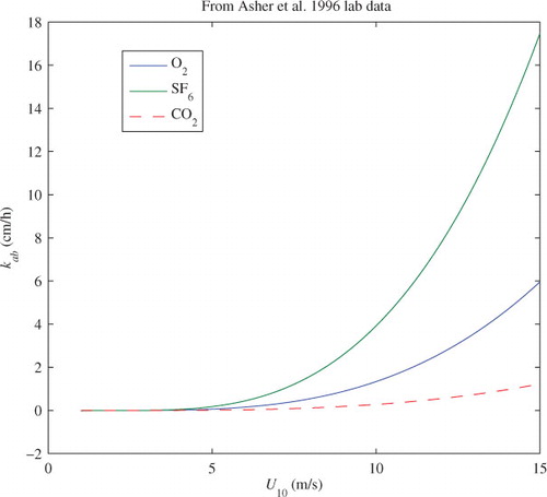This implies that k _ab is assumed to be linearly proportional to the fractional area plume coverage. Furthermore, to extend the laboratory results to field situations, we convert the laboratory fractional area of bubble plume coverage to wind speed via the empirical relation of eq. (23), a practice also employed by Asher et al. (1996). K _ab for SF₆ and O₂ from the minimum mean square error fitting are shown in Fig. 2. Our fitting yields k _ab (SF₆)=2.933k _ab (O₂) at T = 293K. No direct measurements were made to separate injection and exchange transfers in these experiments. However, by scaling arguments, the partition between injection and exchange transfers may be estimated based on measurements of multiple gases (Hamme and Emerson, 2002 2006). Introducing variables for the bubble entrainment rate of small and larger bubbles corresponding to the injection and exchange transfer, and , which are the same for all gases, the asymmetrical transfer velocity is expressed as:17

Fig. 2.  Asymmetric transfer velocities, k _ab , of SF₆, O₂, and CO₂ at 20 °C vs. 10-m wind speed. k _ab is from the regression fitting formula of Asher et al. (1996), Table 3). The laboratory fractional area coverage bubble plume is mapped to the wind speed via eq. (23).

The ratio of can be found from the ratio of the asymmetric transfer velocities of SF₆ and O₂. Likewise, k _ab (CO₂) can be estimated by following the same argument. The minimum possible value of k _ab (CO₂) from the different scaling models of Table 1 is also plotted in Fig. 2. For a reference, k _ab (CO₂)=0.27 cm h⁻¹ at a 10 m height wind speed of 10 m s⁻¹, which can be viewed as a low-bound for k _ab (CO₂) inferred for the experimental set-up. This bound can be further used to check the bound for equilibrium saturation as we will see in the later sections. These experiments are designed mainly to measure the gas transfer velocities. It is true that all the transfer velocities measured in these experiments are not under transfer equilibrium conditions. However, this does not prevent us from deriving the transfer equilibrium saturation from the measured invasion and evasion velocities. To measure the equilibrium saturation directly, one would have to wait until transfer equilibrium is reached, i.e. when net gas transfer becomes zero.

3.3. Global O₂ surface saturation

At the present time, the oceanic O₂ content is climatologically stable despite the annual and decadal variability (Garcia et al., 2005), a fact of the gross long-term balance between changes in O₂ production and respiration, the O₂ solubility pump (thermal), and the air–sea O₂ flux. Could the net surface saturation over climatologic time scale be related to the bubble-mediated gas transfer?

To estimate the average O₂ equilibrium saturation in surface water from surface saturation over climatologic time scale, we employed a 1-D “slab” mixed layer model with vertically homogeneous properties and zero net horizontal exchange:18

where C is the gas concentration in the mixed layer, and h is the mixed layer depth. The three source and sink terms on the right are the air-to-sea gas flux , the local source, P, due to biological and chemical production and consumption, and the bottom flux, , through entrainment and mixing. Horizontal transfer is not important when only a global average transfer is concerned. Such models have been used by Emerson (1987) to study surface O₂ saturation signals due to biological activities and heating in summer warm period at Ocean Weather Station P, and by Keeling et al. (1993) to model air–sea O₂ and N₂ exchange at global scale for the seasonal variations. Surface flux is much larger than the bottom flux, and the combined contributions from the last two terms are assumed to only affect seasonal variability of surface oxygen from a climatological point of view (Keeling et al., 1993). For a reduced system:19

A general solution can be found as (Appendix S2):20

The last term depends on initial conditions and is erased from memory as the system evolves beyond . The second thermal forcing term arises from solubility changes due to the variations in the mixed-layer temperature and in . For example, in summer short warming period, the increase in mixed-layer temperature, T, can be reasonably assumed to vary linearly with time, while is approximately constant (steady wind), Hamme and Emerson (2002) show that:21

and, at seasonal time scales, the rate of temperature change, , can be vary appreciable such that the second thermal forcing term becomes significant. Over a longer time scale, Keeling (1993) points out that this thermal forcing term, as well as the biological contributions, is periodical. Thus, we have demonstrated that, on a global scale, the climatological yearly mean of surface O₂ saturation is approaching to the global mean of equilibrium surface O₂ saturation, .

Calculated based on World Ocean Atlas 2005 data, the climatological yearly mean of surface O₂ saturation is about 1.13%. Our ocean surface average is calculated over a 1 ° by 1 ° grid of climatological monthly mean with its surface temperature above freezing point. The atlas is formed through an objective analysis of all scientifically quality-controlled historical O₂ measurements available in the World Ocean Database 2005 and represents our best knowledge of global dissolved O₂ observations (Garcia et al., 2006). This estimation of the O₂ equilibrium saturation global mean is consistent with other inert gas observations which are of little influenced by biochemical processes. Oceanic observations undertaken around the globe suggest that the degree of ocean surface supersaturation of inert gases (He and Ar) lies in the range of 1–2% (Craig and Hayward, 1987; Spitzer and Jenkins, 1989; Emerson et al., 1991; Schudlich and Emerson, 1996).

This 1–2% range includes gas-mediated transfers from both completely and partially dissolved bubbles (injection- and exchange-type transfers, respectively). These two types of transfers are estimated to be of similar magnitude for O₂, He and Ar (Craig and Hayward, 1987; Schudlich and Emerson, 1996). CO₂ is a much smaller component than O₂ in the atmosphere; therefore, according to the scaling argument, injection-type equilibrium saturation of CO₂ is insignificant. Based on these observations and the conservative scaling argument, the global mean steady-state supersaturation for CO₂ is about 0.15%, probably no less than 0.08%. Here, it is assumed that: (1) the exchange velocity, , is scaled roughly with gas solubility and diffusivity as α^−0.3 D ^0.35 (Keeling, 1993), a conservative scaling model for estimating of CO₂ saturation; and (2) the global mean of exchange type of the O₂ equilibrium saturation is about 0.5%.

4. Data and numerical method

The numerical calculation methods and data used for our estimation of the air–sea CO₂ exchange budget, by asymmetric bubble-mediated gas transfer based on the above parameterisation, are described here. For a given value of , is determined through a global integration which is dependent on the choice of parameterisation model for symmetric gas-transfer velocity, as indicated in the eq. (16). In order to examine the sensitivity of its dependency on , the present calculations include most of the available empirical wind-speed parameterisations of (see list in Table 2). The air–sea CO₂ exchange budget due to asymmetric bubble-mediated gas transfer will be given as percentage of the exchange budget by symmetric gas transfer including both directed surface transfer and bubble-mediated symmetric transfer determined by

Table 2. Surface supersaturation and asymmetric transfer uptakes

			= 0.08%
k s + k out model	k out model	SF sm (Pg C yr^−1)	SF ab /SF sm (%)	(%)	(%)
LM1983	K1993	−0.88	28	0.36	1.4
MS1984	K1993	−0.45	39	0.38	2.1
W1992	K1993	−1.52	28	0.38	0.82
WM1998	K1993	−2.21	19	0.41	0.88
AW1998	AW1998	−1.49	26	0.42	0.94
N2000	K1993	−1.20	29	0.37	1.0
M2002	K1993	−2.40	20	0.44	0.82
MG2001	K1993	−2.07	22	0.44	0.88
MG2004	K1993	−1.19	29	0.43	1.1
Woolf2005	Woolf2005	−1.50	25	0.40	0.94
H2006	K1993	−1.32	28	0.38	1.0

Note: Global CO₂ uptake by bubble-mediated asymmetric transfer for a reference year of 1995. The employed models of symmetrical transfer, k _s + k _out, and bubble-exchange transfer, k _out, are indicated by the corresponding symbols’ reference: LM1983 (Liss and Merlivat, 1983), MS1984 (Monahan and Spillane, 1984), W1992 (Wanninkhof, 1992), K1993 (Keeling, 1993), WM1998 (Wanninkhof and McGillis, 1999), AW1998 (Asher and Wanninkhof, 1998), N2000 (Nightingale et al., 2000), M2002 (Monahan, 2002), MG 2001(McGillis et al., 2001), MG2004 (McGillis et al., 2004), Woolf 2005 (Woolf, 1997, 2005; Woolf et al., 2007), and H2006 (Ho et al., 2006).

.

Among the empirical parameterisations of gas-transfer velocity , the majority of them formulate the transfer velocity as a non-linear relationship of wind speed, u. A few of parameterisations explicitly separate bubble-mediated transfer from transfer via the sea surface (Keeling, 1993; Woolf, 2005; Asher and Wanninkhof, 1998). In these models, bubble transfers are consistently formulated based on the assumption that the bubble-mediated transfer velocity is proportional to fractional whitecap coverage:22

The simplest empirical parameterisation of whitecap coverage of wave breaking is described solely in terms of wind speed and a simple power law (e.g. Monahan and O'Muircheartaigh, 1980; Monahan and Torgensen, 1990; Zhao and Toba, 2001; Asher et al., 2002):23

where n varies between 3 and 4. Such formulas are based mainly on measurements taken from surface optical images. The present study employs, in most cases, n = 3, c ₁ = 1.85 × 10⁻¹, and c ₀ = 2.27, except for the parameterisation models in which is specified (Woolf, 2005; Asher and Wanninkhof, 1998). It has to be pointed out that W(u) here includes only Stage A whitecaps which represent active breaking surfaces. Different choices of parameters, n, c ₁ and c ₀ do not significantly change our conclusion.

The climatological distribution of the ocean surface ΔC _s and the atmospheric C _a of CO₂ for each month over the global oceans were obtained from pCO₂ map series of the ocean surface water and the atmosphere (Takahashi et al., 2002, http://www.ldeo.columbia.edu/res/pi/CO2/). Data with a spatial resolution of 4° × 5° for the year 1995 (the reference year) represent our current state of knowledge regarding pCO₂ of the global surface ocean. The anomalies associated with El Niño periods are excluded from this data set. The data set also contains surface temperature from which the solubility is calculated (Weiss, 1974).

The reference 1995 year atmospheric pCO₂ over the ocean has a strong seasonal cycle in the Northern Hemisphere, but the cycle is much less pronounced in the Southern Hemisphere. This monthly mean of atmospheric pCO₂ is combined with the time series of air sampling from stations located around the globe (http://cdiac.ornl.gov/trends/co2/sio-keel.html) to construct a monthly sequence map of the global atmospheric pCO₂ from 1958 to 2004. Different stations around the world recorded similar annual trends in atmospheric pCO₂, thereby resulting in straightforward interpretations. Since the seasonal change of atmospheric pCO₂ is assumed to follow the trend of the reference year, the inter-annual changes of the atmospheric pCO₂ in a seasonal cycle is not all reflected in our interpreted monthly sequence map of the global atmospheric pCO₂ from 1958 to 2004.

The present analysis employs a 10 m wind speed from a GCM model of the NCEP/NCAR (National Centers for Environmental Prediction/National Center for Atmospheric Research) reanalysis project. All the data is interpolated onto a 4° × 5° low-resolution spatial grid to conform to the resolution of the surface data. To overcome the differences between data of the spatial and temporal means over the grid resolution and local, instantaneous gas-transfer velocity, a wind-speed probability density function (PDF) of the Rayleigh distribution, Pr(u), is adopted. This distribution function is fully specified by the statistical mean value, and has been shown to be a reasonable approximation of the wind-speed frequency distribution for the global ocean (Wentz et al., 1984). Ocean surface temperature from the NCEP/NCAR reanalysis from 1958 to 2004 is also used to calculate the surface solubility. The monthly averaged C _a map is constructed by a multiplication of gas solubility from the reanalysis surface temperature with our interpreted monthly sequence map of the global atmospheric pCO₂ from 1958 to 2004. The part of inter-annual changes of C _a in seasonal cycle due to surface temperature is included in the constructed C _a maps.

Since wind speed at each grid point is specified by its PDF, the gas-transfer velocity, fractional whitecap coverage, and f _e at each grid point i are, therefore, weighted sums of distribution functions of wind speed noted as , and respectively.

is determined numerically according to eq. (16), that is:24

Where S _i is the area of local grid point with its size varying with latitudes. The value of varies with the choices of parameterisation models for and W(u) for a specified value. By the same scheme, the air–sea CO₂ exchange budget of asymmetric bubble-mediated gas transfer, SF _ab , and the total symmetric CO₂ transfer budget, SF _sm , are estimated as follows: 25 and 26

Since SF_as and the ratio, SF_as/SF_sm, are both proportional to , they are also proportional to . There is no need to repeat integral calculation for SF _ab and SF_ab/SF_sm for different values. We have run calculations for different parameterisations for one common value of as listed in Table 2. For other values of , the corresponding values of SF _as /SF _sm can be found proportionally. The first two columns are parameterisation schemes used in our evaluations. The global annual CO₂ budgets of the total symmetric transfer from different models are listed in the third column. The transfer budgets estimated from parameterisations under global constraints, such as the natural-¹⁴C disequilibrium and bomb-¹⁴C inventory, may in fact include both symmetric and asymmetric transfers, even though the flux formulation appears to be symmetric. One of the contributions of this work is to establish a quantitative partition between the contributions from both symmetric and asymmetric transfers. In the subcolumn 1 of column 4, the asymmetric transfer budgets are listed as a percentage of the total transfer budget. In this calculation, we adopted a lower bound of climatologic global-annual-mean of equilibrium saturation:= 0.08%. In the subcolumn 2 of column 4, the equilibrium supersaturation levels from the corresponding parameterisations at a wind speed of 10 m s⁻¹ (at 10 m reference height), f _e ∣₁₀, are also given. For a comparison, listed in the column 5 are the equilibrium supersaturation levels at u = 10 m s⁻¹ calculated with , a value extracted from laboratory experiments (Asher et al., 1996).

5. Results and discussions

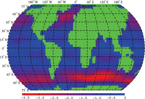
An example of the longitudinally averaged annual mean CO₂ surface supersaturation due to bubble-mediated transfer is shown in Fig. 3. The latitudinal distribution is normalised by the global mean. The longitudinally averaged supersaturation f _e is at its minimum at the equator, and increases toward higher latitudes, in corresponding to the increase in wind speed with latitude. Its rate of change with latitude varies with parameterisation schemes, but the latitudinal increasing trend remains the same. The normalised latitudinal distribution of CO₂ gas equilibrium supersaturation shown in the figure can be extended to the distributions of other gases by a scaling extension. The global distribution of asymmetric gas flux due to bubble-mediated transfer is shown in Fig. 4. Wind-driven asymmetric gas flux due to bubble-mediated transfer increases with increasing wind speed, and has a pronounced effect on CO₂ flux at middle to high latitudes, for example, under the northern and southern storm tracks (Fig. 4).

Fig. 3.  Latitudinal distribution of longitudinally averaged CO₂ equilibrium supersaturation in oceanic surface waters. The symmetric transfer velocity, , used for the calculations (both here and in the other figures) is a quadratic parameterisation of wind speed (Wanninkhof, 1992). If cubic forms of are employed, the maximum supersaturation at high latitudes can exceed three times the global mean.

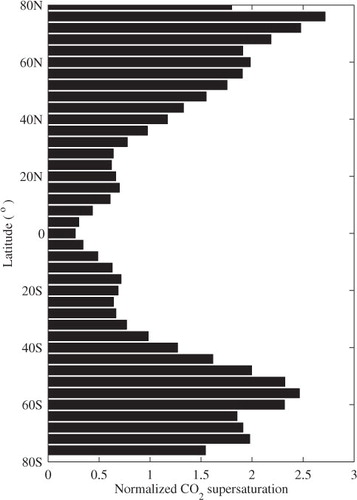
Fig. 4.  Global distribution of bubble-mediated asymmetric CO₂ gas flux. The unit of the linear colour scale is the magnitude of mean global flux; a negative sign indicates a CO₂ ocean sink. Under the constraint of = 0.08%, the mean global flux due to bubble-mediated transfer is 1.3043 g C m ² yr⁻¹.

With a constraint on the global equilibrium supersaturation of CO₂ = 0.08%, our present estimates of the global asymmetric transfer budget of CO₂, SF _as , are on average about 27% of the total of the symmetric global uptake, SF _sm (Table 2). For the CO₂ transfer at sea, locally, asymmetric transfer is insignificant in most cases when compared to the symmetric transfer, for (i.e. f _e is very small). However, the global-integrated bubble-mediated asymmetric transfer is a significant fraction of the total oceanic uptake of the atmospheric CO₂. This is possible because C _a ΔC _s and because ΔC _s changes sign from the low latitudes to the high latitudes while C _a remains relatively constant. The symmetric air–sea uptake SF _sm is negative (i.e. a source to the atmosphere) in the equatorial regions and parts of the tropical oceans, but is positive (a sink) at higher latitudes (Takahashi et al. 2002 2009). The magnitude of the net global flux of symmetric transfer (∣sink∣−∣source∣) is about the same as the magnitude of global SF _sm source (∣source∣), and about a half the magnitude of the global SF _sm sink (∣sink∣).

The variations of global SF _as and SF _sm due to different parameterisation schemes of symmetric transfer are calculated. The ratio of the normalised standard deviation of SF _as to that of SF _sm is about 63%. This suggests that our estimation of SF _as is less sensitive to the parameterisation schemes of symmetric transfer than the estimation of SF _sm is. This reduction of variance is due to the global constraint applied in this case (eq. (16)). However, due to inherently large variation of SF _sm , our result is better to be presented by the ratio of SF _as to SF _sm which is fairly consistent (Table 2). The ratio of SF _as to SF _sm is linearly proportional to the value of the global constraint . To avoid possible overestimation of the asymmetric transfer due to uncertainty of , we chose = 0.08% for the listed results in Table 2.

Regardless of the gas-transfer parameterisation scheme used for the symmetric transfer velocity, , the present calculations reveal that is about 20% of the steady-state saturation for CO₂ at a 10 m s⁻¹ wind speed measured at 10 m above the ocean surface, denoted as f _e ∣₁₀ in Table 2. As we discussed in Section 3, based on the most conservative scaling model and laboratory plume experiments (Asher et al., 1996), the asymmetric transfer velocity for CO₂ is estimated about cm h⁻¹ at a wind speed of 10 m s⁻¹ (10 m reference height). The corresponding equilibrium supersaturations for various models are listed in Table 2 as for comparisons. is consistently about two to three times larger than , the values derived by assuming . Therefore, the constraint of is about a factor of 2 or 3 less than the value inferred from laboratory plume experiments (Asher et al., 1996) if our lab-field conversion is valid. The scaling models of bubble-mediated transfer are essential to our estimation of bounds. We have used the most conservative estimations among bubble transfer models. This topic warrants further thorough investigations for a better assessing the contribution of the asymmetric bubble mediated transfer to the total oceanic uptake budget.

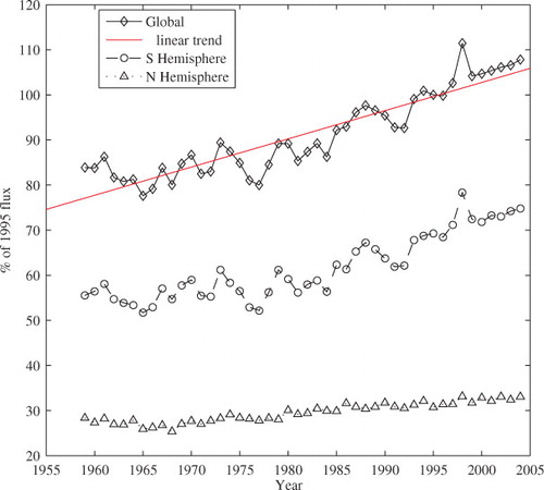
A previous time-trend analysis using deseasonalised surface-water pCO₂ data in parts of the North Atlantic, North and South Pacific, and Southern Oceans (representing about 27% of the global ocean area) indicates that the surface-water pCO₂ over these areas has increased at an average rate of 1.5 µatm yr⁻¹, with basin-specific rates varying between 1.2 ± 0.5 and 2.0 ± 0.4 µatm yr⁻¹ (Takahashi et al. 2009). This result is almost in step with the 0.4–0.5% rate of increase in the atmospheric CO₂ content. Therefore, the change in ΔpCO₂ across the air–sea interface is less than the current increasing rate of the atmospheric CO₂ content. Over times, bubble-mediated asymmetric transfer will represent an increasingly large portion of the total air–sea uptake budget, if the atmosphere and ocean surface water concentrations of CO₂ continue to follow the same similar increasing trends. The bubble-mediated asymmetric transfer would double if the atmosphere CO₂ should double in future. The temporal trend and inter-annual variability of bubble-mediated asymmetric transfer are shown in Fig. 5 with a clear increasing trend. Interannual variability is largely the result of surface wind anomalies in the Southern Hemisphere.

Fig. 5.  Temporal trends in annual ocean CO₂ uptake due to the bubble-mediated asymmetric transfer. Diamonds, circles and triangles represent data of the Global, Southern, and Northern Hemispheres, respectively. The linear fit of the global trend is shown by the solid line. This uptake has increased by almost about 40% in the most recent 50-yr span. The data is normalised by the 1995 reference values. The Northern and Southern Hemispheres fluxes represent 30% and 70% of the 1995 total annual global uptake from bubble-mediated asymmetric transfer.

6. Conclusions

The transfer velocity of bubble-mediated asymmetric transfer is much smaller than transfer velocity of symmetric transfer for CO₂. However, the bubble-mediated asymmetric transfer integrated over long-term periods and large-scale ocean surface contributes to a significant percentage of the total oceanic CO₂ uptake. Moreover, it will become increasingly more important as the atmospheric CO₂ concentration increases. To estimate the global air–sea CO₂ exchange budget from bubble-mediated asymmetric transfer, transfer velocity for the asymmetric transfer is proposed to be proportional to the rate of whitecap coverage. This parameterisation form is synthesised from the results of model simulations and conclusions from bubble distribution observations. The proportionality coefficient, , is constrained by the global mean surface transfer equilibrium saturation . With a value of = 0.08%, we found that the global oceanic uptake from bubble-mediated asymmetric gas transfer is about 20% of the total air–sea CO₂ uptake budget. The value of is deduced by applying scaling relationships to available oceanic observations of gas supersaturation of O₂, H₂, Ar, etc., in ocean surface waters, and a laboratory plume experiment. Being conservative on the uncertainties in estimating the exact value of , our best cautious estimate of the lower bound of is close to 0.1%. Further quantitative studies on scaling properties of bubble mediated gas transfer are needed to reduce these uncertainties. Past debates on the relative importance of gas exchanges via direct surface transfer and via bubble-mediated transfer has been limited mostly to the symmetric transfers only. Within the context of global scale air–sea CO₂ exchange budgets, the asymmetric bubble-mediated transfer adds a significant weight on the importance of bubble-mediated transfer. We have shown analytically that exchange type of bubble-mediated transfer can be approximated by a linear combination of symmetric and asymmetric transfer and they are less sensitive to the gas solubility as some people believed. The parameterisation scheme proposed here can be extended to the transfers of other gases as well. For gases with lower solubility, such as O₂, N₂ and CH₄, small bubbles play a more efficient role in gas exchange. Our assumption of as a constant can be viewed as a first order approximation for the bubble CO₂ transfer models of eq. (9). Dependencies of on wind speed, fetch, and other sea state variables are an important subject of further study.

7. Notations

Table

Subscripts
a	Air
ab	Asymmetric bubble transfer
b	Bubble
e	Transfer equilibrium
f	Final state
i	Initial state
in	Ingassing
o	Climatological yearly mean
out	Outgassing
s	Surface
sm	Symmetric transfer
w	Water
Superscripts
eq	Concentration equilibrium
inj	Injection
exch	Exchange
neq	Concentration non-equilibrium
*	Non-dimensional
Main symbols
B	Bubble size and depth distribution density
C	Gas concentration
D	Molecular diffusivity
f	Supersaturation
F	Flux
g	Gravitational acceleration
h	Mixed layer depth
j	Individual bubble gas transfer velocity
k	Gas transfer velocity
L	Individual bubble trajectory
n	Molar content of a tracer gas contained in individual bubble
N	Total transfer of a tracer gas by an individual bubble during its lifetime in water
𝒩	Molar content of all tracer gases contained in an individual bubble
p	Pressure; pCO2 is CO2 partial pressure
P	Total pressure
r	Bubble radius
R	Ideal gas constant
S	Surface area of an individual bubble
SF	Regional uptakes: integrated flux over an area
t	Time
T	Temperature
u	Wind speed at the 10 m reference height
V	Volume
w	Vertical velocity
W	Fractional whitecap coverage factor
z	Depth
α	Gas solubility
β	Ostwald solubility coefficient
Δ	Difference or increment; ΔpCO2 is CO2 partial pressure difference, and ΔT is temperature increment.
γ	Surface tension
Φ	Bubble source distribution function
Σ	rate of volume entrainment
ν	Viscosity

8. Acknowledgements

Author is indebted to Prof. R. Keeling for suggesting to use available oxygen data for estimating transfer equilibrium of surface gas saturations. Support from the National Science Foundation (grant no. OCE06477819) and UCSD academic senator are acknowledged.

9. Appendix S1

9.1. Decomposition of bubble transfer

For a spherical bubble, the Fickian flux equation for the rate of its tracer gas molar content change is:A1

where n is the molar content of tracer gas in the bubble, and r is the bubble radius. The dependency of individual bubble transfer velocity, j, on the molecular diffusivity, D, varies with Reynolds number, Re (Levich, 1962; Thorpe, 1982; Woolf and Thorpe, 1991). For example, clean bubble gas transfer velocity is:A2

where w _b is the bubble rising speed. For bubble radii larger than 0.004 cm, Re>1. Applying the ideal gas law and derivation chain rule , we have:A3

where R is ideal gas constant, and p _b is partial bubble gas pressures. T and V are the bubble volume and temperature. The vertical axis z points upward with origin at the water surface. Vertical velocity, w, equals bubble terminal speed and vertical advection velocity by background flows. Also, j is replaced by D ^d ν ^1/2−d j* in order to factorise out the chemo-physical parameter. The exponent constant, d, is either 2/3 or 1/2 depend on bubble's Reynolds number. The volume of bubble varies with depth due to hydrostatic expansion and compression and with the change in total molar content of all gases _: A4

P _b is the total bubble gas pressures, P _a is the atmosphere pressure at sea surface, and γ is surface tension of seawater. Both V and are related to n, so the eq. (A3) is non-linear. When dissolution is small, like for large bubbles, the volume change is mainly controlled by hydrostatic expansion and compression, then:A5

where V _i is initial volume of the bubble. It follows that:

With:

andA6

where , and . The solution of the linearised eq. (A6) is:A7

The total molar gas exchanged during the bubble life time is:A8

where n _f is the remaining molar gas content within the bubble when it comes back to the surface. After some manipulating of the integral by parts, we arrive at:A9

where V _f is the volume of bubble back at water surface. Note here that the gas chemo-physical parameter θ only appears in exponential components and is proportional to both air and water gas concentration, C _a and C _w . We define:A10

We proof here that, in general, for an individual bubble can be separated into symmetric and asymmetric parts under the linear approximation which ignores bubble volume change associated with gas dissolution:A11

10. Appendix S2

10.1. Mixed layer model for gas concentrations of climatologically balanced gases in ocean surface water

Considering a 1-D ocean mixed layer model as an approximation for horizontally averaged surface gas inventory,A12

where P is the net local productions and consumptions, is the surface gas flux, and is the flux into ocean below across thermalcline. Oceanic O₂ inventory has been stable on time scales of years to centuries. The rate of change in oceanic O₂ inventory equals to sea-to-air O₂ flux and the oceanic inventory of organic carbon (Keeling and Garcia, 2002). Total ocean column-integrated net production of O₂ by marine photosynthesis and respiration and mixed-layer bottom fluxes is presumably much smaller than the sea-to-air O₂ flux. This is because the main effect of marine photosynthesis and respiration on these time scales is to redistribute inorganic materials within the ocean rather than to cause accumulation or destruction of organic carbon within the ocean surface layer. Therefore, omitting the last two terms on the right, we have a linear surface inventory equation:A13

Its general solution is:A14

It can be found, through integrating by parts, that:A15

Rewriting the solution in terms of surface saturation, yields:A16

References

- Asher, W. E, Edson, J. B, McGillis, W. R, Wanninkhof, R, Ho, D. T. and co-authors. 2002. Fractional area whitecap coverage and air–sea gas transfer during GasEx-98. In: Gas Transfer at Water Surfaces. ( M. A.Donelan, W. M.Drennan, E. S.Saltzman and R.Wanninkhof). American Geophysical Union: Washington DC, pp. 199–204.
- Asher W. E, Karle L. M, Higgins B. J, Farley P. H, Monahan E. C, co-authors.. The influence of bubble plumes on air/seawater gas transfer velocities. J. Geophys. Res. 1996; 101: 12027–12042. 10.3402/tellusb.v64i0.17260.
- Asher W. E, Wanninkhof R. The effect of bubble-mediated gas transfer on purposeful dual gaseous-tracer experiments. J. Geophys. Res. 1998; 103: 10555–10560. 10.3402/tellusb.v64i0.17260.
- Caldeira K, Wickett M. E. Anthropogenic carbon and ocean pH. Nature. 2003; 425: 365–365. 10.3402/tellusb.v64i0.17260.
- Cipriano R. J, Blanchard D. C. Bubble and aerosol spectra produced by a laboratory ‘breaking wave’. J. Geophys. Res. 1981; 86: 8085–8092. 10.3402/tellusb.v64i0.17260.
- Craig H, Hayward T. Oxygen supersaturation in the ocean: biological versus physical contributions. Science. 1987; 235: 199–235. 10.3402/tellusb.v64i0.17260.
- Craig H, Weiss R. F. Dissolved gas saturation anomalies and excess helium in the ocean. Earth Planet. Sci. Letts. 1971; 10: 289–296. 10.3402/tellusb.v64i0.17260.
- Crawford G. B, Farmer D. M. On the spatial distribution of bubbles generated by breaking waves. J. Geophys. Res. 1987; 92(C8): 8231–8242. 10.3402/tellusb.v64i0.17260.
- Deane G. B, Stokes D. Scale dependence of bubble creation mechanisms in breaking waves. Nature. 2002; 418: 839–844. 10.3402/tellusb.v64i0.17260.
- Emerson S. Seasonal oxygen cycles and biological new production in surface water of the subarctic Pacific Ocean. J. Geophys. Res. 1987; 92: 6535–6544. 10.3402/tellusb.v64i0.17260.
- Emerson S, Quay P, Stump C, Wilbur D, Knox M. O2, Ar, N2 and 222Rn in surface water of the subarctic Pacific Ocean: net biological O2 production. Global Biogeochem. Cycl. 1991; 5: 49–69. 10.3402/tellusb.v64i0.17260.
- Erickson D. J, Merril J. T, Duce R. A. Seasonal estimates of global oceanic whitecap coverage. J. Geophys. Res. 1986; 91: 12975–12977. 10.3402/tellusb.v64i0.17260.
- Fairall C. W, Hare J. E, Edson J. B, McGillis W. R. Parameterization and micrometeorological measurement of air-sea gas transfer. Science. 2000; 96: 63–105.
- Feely R. A, Sabine C. L, Lee K, Berelson W, Kleypas J, co-authors.. Impact of anthropogenic CO2 on the CaCO3 system in the oceans. J. Geophys. Res. 2004; 305: 362–366. 10.3402/tellusb.v64i0.17260.
- Fuchs G, Roether W, Schlosser P. Excess 3He in the ocean surface layer. Geophys. Res. Lett. 1987; 92: 6559–6568. 10.3402/tellusb.v64i0.17260.
- Garcia, H. E, Boyer, T. P, Levitus, S, Locarnini, R. A and Antonov, J. 2005. On the variability of dissolved oxygen and apparent oxygen utilization content for the upper world ocean: 1955 to 1998. 32: L09604. 10.3402/tellusb.v64i0.17260.
- Garcia, H. E, Locarnini, R. A, Boyer, T. P and Antonov, J. I. 2006. World Ocean Atlas 2005, Volume 3: Dissolved Oxygen, Apparent Oxygen Utilization, and Oxygen Saturation. (S.Levitus). NOAA Atlas NESDIS 63: U.S. Government Printing OfficeWashington, DC, 342. pp.
- Hamme, R. C and Emerson, S. R. 2002. Mechanisms controlling the global oceanic distribution of the inert gases argon, nitrogen and neon. J. Mar. Res. 29(23): 2120. 10.3402/tellusb.v64i0.17260.
- Hamme R. C, Emerson S. R. Constraining bubble dynamics and mixing with dissolved gases: implications for productivity measurements by oxygen mass balance. Geophys. Res. Lett. 2006; 64(1): 73–95. 10.3402/tellusb.v64i0.17260.
- Ho D. T, Law C. S, Smith M. J, Schlosser P, Harvey M, co-authors.. Measurements of air–sea gas exchange at high wind speeds in the Southern Ocean: implications for global parameterizations. J. Phys. Oceanogr. 2006; 33: L16611.10.3402/tellusb.v64i0.17260.
- Hwang P. A, Hsu Y. H. L, Wu J. Air bubbles produced by breaking wind waves: a laboratory study. J. Geophys. Res. 1990; 20: 19–28.
- Jenkins W. J. The use of anthropogenic tritium and helium-3 to study subtropical gyre ventilation and circulation. J. Mar. Res. 1988; A 325: 43–61. 10.3402/tellusb.v64i0.17260.
- Jähne B, Münnich K. O, Bösinger R, Dutzi A, Huber W, co-authors.. On the parameters influencing air–water gas exchange. Proc. USA Natl. Acad. Sci. 1987; 92: 1937–1949. 10.3402/tellusb.v64i0.17260.
- Keeling R. F. Role of bubbles in air–sea gas exchange. Global Biogeochem. Cycles. 1993; 51: 237–271. 10.3402/tellusb.v64i0.17260.
- Keeling R. F, Garcia H. E. The change in oceanic O2 inventory associated with recent global warwing. Nature. 2002; 99: 7848–7853. 10.3402/tellusb.v64i0.17260.
- Keeling R. F, Najjar R. P, Bender M. L, Tans P. P. What atmospheric oxygen measurements can tell us about the global carbon cycle. Tellus. 1993; 7: 37–67. 10.3402/tellusb.v64i0.17260.
- Keeling R. F, Piper S. C, Heimann M. Global and hemispheric CO2 sinks deduced from changes in atmospheric O2 concentration. Oceanology. 1996; 381: 218–221. 10.3402/tellusb.v64i0.17260.
- Koga M. Bubble entrainment in breaking wind waves. Nature. 1982; 34: 481–489. 10.3402/tellusb.v64i0.17260.
- Kolovayev P. A. Investigation of the concentration and statistical size distribution of wind-produced bubbles in the near-surface ocean layer. 1976; 15: 659–661.
- Lamarre E, Melville W. K. Air entrainment and dissipation in breaking waves. 1991; 351: 469–472. 10.3402/tellusb.v64i0.17260.
- Lee K, Wanninkhof R, Takahashi T, Doney S. C, Feely R. A. Low interannual variability in recent oceanic uptake of atmospheric carbon dioxide. Marine Chem. 1998; 396: 155–159. 10.3402/tellusb.v64i0.17260.
- Levich V. G. Physicochemical Hydrodynamics. Prentice-Hall: Englewood Cliffs NJ, 1962
- Liss, P. S and Merlivat, L. 1983. Air–sea gas exchange rates: introduction and synthesis. In: The Role of Air–sea Exchange in Geochemical Cycling. (P.Buat-Menard). Reidel Publishing Co.: Dordrecht, pp. 113–129.
- McGillis W. R, Edson J. B, Ware J. D, Dacey J. W. H, Hare J. E, co-authors.. Carbon dioxide flux techniques performed during GasEx-98. J. Mar. Sys. 2001; 75: 267–280. 10.3402/tellusb.v64i0.17260.
- McGillis, W. R, Edson, J. B, Zappa, C. J, Ware, J. D, McKenna, S. P. and co-authors. 2004. Air–sea CO2 exchange in the equatorial Pacific. Tellus. 109(C08S02): 10.3402/tellusb.v64i0.17260.
- McNeil C, D'Asro E. Parameterization of air–sea gas fluxes at extreme wind speeds. J. Geophys. Res. 2007; 66: 110–121. 10.3402/tellusb.v64i0.17260.
- Melville W. K. The role of surface-wave breaking in air-sea interaction. 1996; 28: 279–321. 10.3402/tellusb.v64i0.17260.
- Memery L, Merliva L. Modelling of gas flux through bubbles at the air–water interface. J. Phys. Oceanogr. 1985; 37B: 272–285. 10.3402/tellusb.v64i0.17260.
- Merlivat L, Memery L. Gas exchange across an air–water interface: experimental results and modeling of bubble contribution to transfer. 1983; 88: 707–724. 10.3402/tellusb.v64i0.17260.
- Monahan E. C. 2002. The physical and practical implications of a CO2 gas transfer coefficient that varies as the Cube of wind speed. In: Gas Transfer at Water Surfaces. (M. A.Donelan, W. M.Drennan, E. S.Saltzman and R.Wanninkhof). American Geophysical Union: Washington DC, pp. 193–197.
- Monahan E. C, O'Muircheartaigh I. G. Optimal power-law description of oceanic whitecap coverage dependence on wind speed. J. Geophys. Res. 1980; 10: 2094–2099.
- Monahan, E. C and Spillane, M. C. 1984. The role of oceanic whitecaps in air–sea gas exchange. In: Gas Transfer at Water Surfaces . (W.Brutsaert and G. H.Jiaka). Reidel Publishing Co.: Dordrecht, pp. 495–503.
- Monahan, E. C and Torgersen, T. 1990. The enhancement of air–sea gas exchange by oceanic whitecapping. In: Air–Water Mass Transfer. (S. C.Wilhelms and J. S.Gulliver). American Society of Civil Engineers: New YorkNY, pp. 608–617.
- Monahan E. C, Zeitlow C. R. Laboratory comparisons of fresh-water and salt-water whitecaps. 1969; 74: 6961–6966. 10.3402/tellusb.v64i0.17260.
- Nightingale P. D, Malin G, Law C. S, Watson A. J, Liss P. S, co-authors.. In situ evaluation of air–sea gas exchange parameterizations using novel conservative and volatile tracers. 2000; 14: 373–387. 10.3402/tellusb.v64i0.17260.
- Orr J. C, Fabry V. J, Aumont O, Bopp L, Doney S. C, co-authors.. Anthropogenic ocean acidification over the twenty-first century and its impact on calcifying organisms. Science. 2005; 437: 681–686. 10.3402/tellusb.v64i0.17260.
- Prentice, I. C. 2001. The carbon cycle and atmospheric carbon dioxide. In: Climate Change 2001: The Scientific Basis. Contribution of Working Group I to the Third Assessment of the Intergovernmental Panel on Climate Changes. (J. T.Houghton, Y.Ding, D.J.Griggs, M.Noguer, P.J.van der Linden, X.Dai, K.Maskell, and C.A.Johnson). Cambridge University Press: New YorkNY, pp. 183–237.
- Sabine C. L, Feely R. A, Gruber N, Key R. M, Lee K, co-authors.. The oceanic sink for anthropogenic CO2. Deep-Sea Res. II. 2004; 305: 367–371. 10.3402/tellusb.v64i0.17260.
- Sarmiento J. L, Gruber N. Sinks for anthropogenic carbon. J. Phys. Oceanogr. 2002; 55(8): 30–36. 10.3402/tellusb.v64i0.17260.
- Schudlich B, Emerson S. Gas supersaturation in the surface ocean: the roles of heat flux, gas exchange, and bubbles. J. Mar. Res. 1996; 43: 569–589. 10.3402/tellusb.v64i0.17260.
- Soloviev A. V, Schlüssel P. Parameterization of the temperature difference across the cool skin of the ocean and of the air–ocean gas transfer on the basis of modelling surface renewal. Deep-Sea Res. II. 1994; 24: 1339–1346.
- Spitzer W. S, Jenkins W. J. Rates of vertical mixing, gas exchange, and new production: estimations from seasonal gas cycles in the upper ocean near Bermuda. Deep-Sea Res. II. 1989; 47: 169–196. 10.3402/tellusb.v64i0.17260.
- Takahashi T, Sutherland S. C, Sweeney C, Poisson A, Metzl N, co-authors.. Global sea-air CO2 flux based on climatological surface ocean pCO2, and seasonal biological and temperature effects. 2002; 49: 1601–1622. 10.3402/tellusb.v64i0.17260.
- Takahashi, T, Sutherland, S. C, Wanninkhof, R. ,Sweeney, C, Feely, R. A. and co authors. . 2009. Climatological mean and decadal changes in surface ocean pCO2, and net sea-air CO2 flux over the global oceans. Phil. Trans. Royal Soc. London. 56: 554–577.
- Thorpe S. A. On the role of clouds of bubbles formed by breaking waves in deep water and their role in air–sea gas transfer. 1982; A304: 155–210.
- Wanninkhof R. Relationship between wind speed and gas exchange over the ocean. J. Geophys. Res. 1992; 97: 7373–7382. 10.3402/tellusb.v64i0.17260.
- Wanninkhof R, Asher W. E, Ho D. T, Sweeney C, McGillis W. R. Advances in quantifying air–sea gas exchange and environmental forcing. Ann. Rev. Marine Sci. 2009; 1: 213–244. 10.3402/tellusb.v64i0.17260.
- Wanninkhof R, McGillis W. M. A cubic relationship between gas transfer and windspeed. Geophys. Res. Lett. 1999; 26: 1889–1892. 10.3402/tellusb.v64i0.17260.
- Weiss R. F. Carbon dioxide in water and seawater: the solution of a non-ideal gas. Mar. Chem. 1974; 2: 203–215. 10.3402/tellusb.v64i0.17260.
- Wentz F. J, Peteherch S, Thomas L. A. A model function for ocean radar cross section at 14.6 Ghz. J. Geophys. Res. 1984; 89: 3689–3704. 10.3402/tellusb.v64i0.17260.
- Woolf, D. K. 1997. Bubbles and their role in air–sea gas exchange. In: The Sea Surface and Global Change. (Liss, P. S. and Duce, R. A.). Cambridge University Press. pp. 173–205.
- Woolf D. K. Parameterization of gas transfer velocities and sea-state-dependent wave breaking. Tellus. 2005; 57B: 87–94.
- Woolf D. K, Thorpe S. A. Bubbles and the air–sea exchange of gases in near-saturation conditions. J. Mar. Res. 1991; 49: 435–466. 10.3402/tellusb.v64i0.17260.
- Woolf D. K, Leifer I. S, Nightingale P. D, Rhee T. S, Bowyer P, co-authors.. Modelling of bubble-mediated gas transfer: fundamental principles and a laboratory test. J. Mar. Sys. 2007; 66: 71–91. 10.3402/tellusb.v64i0.17260.
- Zhao D, Toba Y. Dependence of whitecap coverage on wind and wind-wave properties. 2001; 57: 603–616. 10.3402/tellusb.v64i0.17260.