A year of H₂ measurements at Weybourne Atmospheric Observatory, UK

ABSTRACT

We present a year-long high precision time series of atmospheric molecular hydrogen (H₂) measured at the UK North Sea coast from March 2008 to February 2009. We observed a pronounced seasonal cycle in H₂ with mean values in late winter/early spring~40 ppb higher than those in late summer/early autumn. Background-subtracted molar H₂/CO ratios (ΔH₂/ΔCO) averaged 0.35±0.002 for all data combined and 0.25±0.002 when ΔH₂ was above 10 ppb. The ΔH₂/ΔCO ratio was highest in summer, possibly as a result of larger photochemical production. Using simultaneous measurements of ozone, we estimated the deposition velocity of H₂ during nocturnal inversion events to average 3.5±0.7×10⁻⁴ m s⁻¹ for June 2008 and 1.9±1×10⁻⁴ m s⁻¹ for July 2008, in good agreement with other reported estimates. In May 2008, we observed an episode of exceptionally clean air being transported from the tropics but arriving from the north, in which H₂ was slightly elevated indicating minimal surface loss. On another occasion with south-easterly winds, we believe we detected emissions from H₂ production facilities in the near-continent characterised by H₂ mixing ratios reaching 1450 ppb.

• H₂
• molecular hydrogen
• H₂/CO ratios
• deposition velocity
• carbon monoxide

1. Introduction

Atmospheric molecular hydrogen (H₂) is present in the Earth's atmosphere at approximately 530 ppb (Novelli et al., 1999), making it the second most abundant reduced gas in the atmosphere after methane (CH₄). In recent years, atmospheric H₂ has received increased attention due to its promising future as an energy carrier. However, such an H₂-based economy may impact the Earth's atmosphere as a result of increased levels of H₂ in the atmosphere due to leakage during transport and distribution processes. Possible future perturbations include a reduction in atmospheric oxidising capacity through a reduction of tropospheric hydroxyl radical (OH) (Schultz et al., 2003; Warwick et al., 2004) and increases in stratospheric water vapour, which could lead to enhanced stratospheric ozone (O₃) destruction (Tromp et al., 2003). H₂ is considered an indirect greenhouse gas (Derwent et al., 2006).

Several studies have investigated the strengths of the various terms that make up the tropospheric H₂ budget (Novelli et al., 1999; Hauglustaine and Ehhalt, 2002; Sanderson et al., 2003; Rhee et al., 2006; Price et al., 2007; Xiao et al., 2007; Ehhalt and Rohrer, 2009; Pieterse et al., 2011; Yashiro et al., 2011) and are summarised in Pieterse et al. (2011). In summary, estimates of the tropospheric burden of H₂ range from 136 to 157 Tg H₂. The dominant source in this budget is considered to be from the oxidation of methane (CH₄) and non-methane hydrocarbons, which together account for~50% of the total, with biomass burning (~20%), fossil fuel emissions (~20%) and nitrogen fixation (~10%) making up the remainder.

There will also be some contribution to ambient H₂ from industry. Hydrogen is both consumed and produced from a wide variety of processes, with the potential for fugitive release in all cases, although by what amount is almost unknown and liable to be highly variable. Further fugitive releases are possible during transport, transfer and storage. In Europe, it is refineries and ammonia production that together account for around 82% of consumption, with smaller amounts used in methanol production, the metal industry and a plethora of minor uses (Maisonnier and Perrin, 2007). Production is largely onsite production as fuel and feedstock for the above industries (64% of European total production), with a further 27% as by-product notably from the chemical industry and cokeovens. In Europe, production is geographically concentrated in the Benelux and Rhein-Main area, as well as the North East and Midlands of the UK, and northern Italy (Maisonnier and Perrin, 2007). Germany is the largest H₂ producer in Europe followed by the Netherlands and the UK.

The sinks for H₂ are deposition to the soils and the reaction with the hydroxyl radical (OH) with the former accounting for~70–80% of the total sink. Estimates of the total loss of H₂ versus the tropospheric burden yield a H₂ tropospheric lifetime between 1.4 and 2.1 yr. At present, it remains uncertain whether the tropospheric H₂ mixing ratio is increasing or decreasing with some studies reporting increasing trends (Khalil and Rasmussen, 1990; Simmonds et al., 2000) and some decreasing trends (Novelli et al., 1999; Bond et al., 2011). Grant et al. (2010b) report that the annual average atmospheric mixing ratio of H₂ has remained stable over a 15-year period from observations at Mace Head, Ireland.

Continuous measurements of H₂ in air were made at the Weybourne Atmospheric Observatory (hereafter Weybourne), UK, as part of the EU-funded EuroHydros (European Network for Atmospheric Hydrogen Observations and Studies) project whose principle aim was to set up a continuous H₂ monitoring network across Europe (e.g. Yver et al., 2011). Here, we discuss some special features of the measurements made at this coastal observing station on the North Sea, over the course of a year.

2. Experimental methodology

2.1. Site description

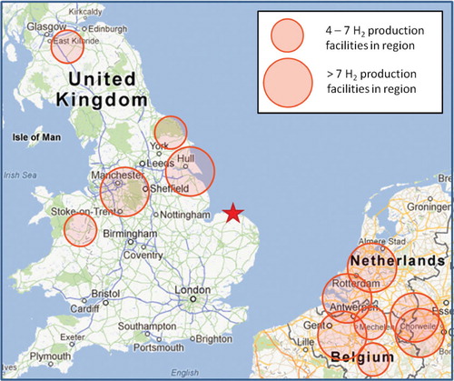
Measurements of H₂ and CO were performed at Weybourne from March 2008 to February 2009. Weybourne is located on the North Norfolk coast (52.95°N, 1.13°E, Fig. 1) (Penkett et al., 1999). The station experiences air masses from a range of sources including relatively clean maritime air, continental Europe and polluted UK air masses. It is located approximately 170 km north east of London and 200 km due east of Birmingham.

Fig. 1.  Map showing the location of Weybourne Atmospheric Observatory (red star). Major centres of H₂ production (four facilities and over) in the UK and the Benelux region are highlighted using semi-transparent red circles. Map Source: Google Maps.

The station is equipped with a full meteorological suite including sonic anemometer and a Sonic Detection and Ranging-Radio-Acoustic Sounding System (SODAR-RASS). In addition to H₂ and CO, the station is also responsible for high frequency measurements of other tropospheric constituents including NO_x (NO and NO₂), ozone (O₃) and condensation nuclei (CN). Air is drawn rapidly through a large glass tube from an inlet on a tower at 10 m a.g.l. (25 m a.s.l.) and circulated through the laboratory via a glass manifold from which subsequent air samples are collected and analysed.

2.2. Determination of H₂ and CO mixing ratios

Routine analysis of H₂ was achieved using a modified commercial Reduction Gas Analyser (RGA3, Trace Analytical, Inc., California, USA), which includes gas chromatography followed by the reduction of mercuric oxide. Mercury vapour from this reaction was detected by UV absorption. The first step in the gas chromatography was the removal of H₂O, CO₂ and hydrocarbons using a pre-column consisting of Unibeads 1S (mesh 60/80; 1/8 in. OD×76 cm length). This step was immediately followed by the separation of H₂ from CO using molecular sieve 5A (mesh 60/80; 1/8 in. OD×76 cm length). Synthetic air (BTCA air 178, British Oxygen Company, UK) was used as a carrier gas with a flow of 17 cm³ min⁻¹. Prior to entering the system, the carrier gas was passed through traps containing molecular sieve 5A to remove H₂O preceded by removal of CO and H₂ using SOFNOCAT 514 (Molecular Products Ltd). Columns were maintained at a constant temperature of 92°C and detector temperature was maintained at 265°C.

Air was drawn from the glass manifold mentioned in Section 2.1 using PTFE tubing (1/4 in. OD×76 cm length) at a rate of 200 cm³ min⁻¹ using an air pump downstream of the sample loop. The air was passed through a moisture trap (silica beads) before entering a 1-cm³ sample loop. The air pump was turned off 20 s prior to sample injection to allow pressure equilibration of the sample loop. The pressure and the temperature of the sample loop were monitored throughout analysis using a pressure sensor (Setra 278 Barometer) and temperature sensor (NOVUS TxRail 0–10Vdc), respectively. A run time of 6 min allows eight air samples to be analysed every hour with a working standard analysed after every fourth run. This resulted in eight fully calibrated measurements of H₂ and CO each hour. Detector response, sample loop pressure and temperature were all recorded using a six-channel analogue to digital acquisition system (Model 302, SRI Instruments, California, USA) and subsequent peak analysis was performed using Peak Simple software (SRI Instruments). Peak heights measured from samples were referenced to a working standard with close to ambient mixing ratios of H₂ and CO, which were calibrated at Max Planck Institute-Jena with reference to the MPI-2009 scale for H₂ (Jordan and Steinberg, 2011) and NOAA2004 scale for CO.

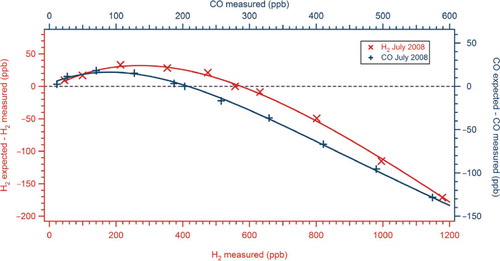
System non-linearity was quantified by dynamic dilution of a high concentration H₂ and CO standard (BOC) with BTCA 178 air (BOC) scrubbed using SOFNOCAT 514 to remove any H₂ and CO. The non-linear response curve generated was then checked against standards calibrated at MPI-Jena. For example, for H₂, the agreement between dilution and working tank was typically within 1% for a working standard containing 561 ppb and within 2% for a working tank containing 1001 ppb. For CO, the agreement was within 2% for a working standard containing 205 ppb. The agreement between the H₂ working standards and the dilutions gave us confidence that our dilution was linear and that any non-linearity was caused by the detector response to H₂ and CO. Figure 2 shows the detector non-linearity for H₂ and CO determined in July 2008. Peak heights measured from samples were normalised to the non-linear response function using the mean relative response of the working standard determined at 30-min intervals. System precision was assessed using repeat analysis of a standard with close to ambient mixing ratios. During this test, the standard was run every 6 min over a 1-h period and routinely showed< 1% variation (1σ) for H₂ and< 2% (1σ) for CO.

Fig. 2.  Example of RGA3 non-linearity results for July 2008. ‘H₂ expected’ is the mixing ratio expected from a linear relationship determined from a single point calibration and this point lies on the dashed line.

Quality assurance was carried out during two separate intercomparison exercises. The first of these was performed in June 2008 within the framework of the EuroHydros project and consisted of analysing four canisters with known H₂ mixing ratios (spanning 490–650 ppb). These four canisters were circulated between the EuroHydros partners and each partner determined the H₂ mixing ratio in each canister. These results from each laboratory were then compared with the H₂ mixing ratios determined at MPI-Jena. The H₂ mixing ratio determined using our system for each canister was within 1.4% (estimated from 1% uncertainty for each laboratory) of those determined at MPI-Jena. The second exercise was part of the ‘Cucumbers’ intercomparison programme supported through CarboEurope (Manning et al., 2009). In October 2008, we analysed three canisters circulating as part of the “Inter-1” loop for H₂ and CO mixing ratios in the range 529–536 ppb and 145–180 ppb, respectively. Our average offsets from the mixing ratios determined at MPI-Jena were 0.44±1.74 ppb and− 0.92±0.51 ppb for H₂ and CO, respectively. This was within the World Meteorological Organisations (WMO) intercomparability goal of ±2 ppb for H₂ and CO.

2.3. Supplementary chemical measurements

A range of supplementary chemical measurements were available at Weybourne, which were used to aid the interpretation of the H₂ measurements. Nitric oxide (NO) and nitrogen dioxide (NO₂) were measured using a chemiluminescence technique (ThermoScientific; model TE42C). Using this technique, NO₂ is converted to NO using a molybdenum convertor operated at 325°C. However, as the molybdenum convertor is not specific to NO₂, the NO_x measurements include total reactive nitrogen (NO_y). Ozone (O₃) measurements were performed with a commercial gas analyser (ThermoScientific; model TE49C), which measures the UV absorption of O₃ at 254 nm. Condensation nuclei counts were measured with a TSI model 3022A counter (cutoff size 0.007 µm).

2.4. Meteorological data

Meteorological data were obtained using two separate systems. The first of which was an automatic meteorological station (AWS, Campbell Scientific), which measured ambient air temperature, relative humidity, wind speed, wind direction and direct and diffuse solar irradiance. In addition, meteorological parameters were measured using an ultrasonic anemometer, which provided a range of parameters including mean windspeed, wind fluctuations at 10 Hz, wind direction, temperature and vertical heat and momentum flux (METEK GmbH, Germany).

2.5. SODAR-RASS

The METEK RASS DSDPA-90 used in this study consisted of a phased-array SODAR using an acoustic frequency of 1500–4000 Hz, a height resolution of 20 m and a maximum range of about 400 m. The acoustic signal propagation was observed by a two-antenna radar system working continuously at 1290 MHz with a power of 20 W. The emitting antenna was placed 0.5 m upstream of the SODAR, the receiving antenna 0.5 m downstream. Data analysis provided the temperature profile up to 400 m at 20 m height resolution with an accuracy of 0.3 K. Additionally, the Doppler-RASS delivers also delivered vertical profiles of the wind vector, the standard deviation of the vertical wind component and the acoustic backscatter intensity. This information was converted into a temperature profile up to several hundreds of metres above ground level. An overview of the algorithms used for the determination of mixing-layer height from remote sensing devices may be found in Emeis et al. (2008).

2.6. NAME model setup

For interpreting the air mass history in this study, the UK Met office's NAME dispersion model (Ryall et al., 2001) with Unified Model meteorological data was run in backwards mode as illustrated for composition measurements at Weybourne in Fleming et al. (2012). The model follows the release of thousands of inert particles (10 000 per hour in this case), for two scenarios: 10-day backwards in time for 3 hourly release periods tracking the particle's latitude and longitude at both 0–100 m and 0–1000 m altitude ranges and 2-day backwards in time for hourly release periods for the 0–100 m altitude range, which will detect when the air mass has been in contact with surface emissions. The particles in the model were released from the height of the sample inlet on the station's tower. The spatial resolution was 0.05°×0.05° for the 2-day and 0.25°×0.25° for the 10-day domains. The resulting plots derived from NAME can be considered as air mass footprints highlighting the probability of where air masses arriving at the site had passed during the preceding 2- or 10-day period.

3. Results and discussion

3.1. General observations

Figure 3 shows the time-series of H₂ measured at Weybourne from March 2008 to February 2009 and consists of approximately 57 000 data points. Note the change in axis scale at mixing ratios above 800 ppb. The data show a minimum H₂ value of 423 ppb with a maximum value of 1450 ppb and a mean (±one sigma standard deviation) of 515 ppb±22 ppb. It was rare for the H₂ mixing ratio to exceed 600 ppb, and this was reflected in a value of 565 ppb for the 99th percentile. The second highest H₂ event had a maximum of 677 ppb, and this value was more comparable to maximum values recorded at other remote sites. For example, it compares with the range (when converted from the CSIRO scale to the MPI-2009 scale) observed at Mace Head over a 15-year period of 436.9 to 658.5 ppb with a mean (±one sigma standard deviation) of 519±17.6 ppb (Grant et al., 2010b). The largest of the positive excursions may relate to specific sources (Section 3.6), whilst in other cases they evidently represent more generally polluted conditions (Section 3.5).

Fig. 3.  Time series of H₂ measured at Weybourne for period March 2008–February 2009. Note the change in axis scale above 800 ppb. The red markers represent the background H₂ estimated in Section 3.1.

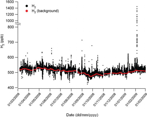
An additional dominant feature visible in Fig. 3 is the negative excursions in the H₂ time-series. These were more evident during the first part of the record, and notably so during the late spring and summer months, May to August, and were largely absent from October through to the following February. These excursions we believe were a result of deposition of H₂ to the soil and are considered in more detail in Section 3.7.

The red line in Fig. 3 represents the ‘background’ or ‘baseline’ mixing ratios of H₂. We estimated these background mixing ratios of H₂ by calculating a running quantile probability of 0.2 with an interval size of 10 d (Barnes et al., 2003a). Sensitivity tests with varying interval sizes (2–30 d) and quantile probabilities (0.1–0.3) were carried out, and the chosen parameters deemed to best capture the background of H₂ without bias towards either pollution events or soil deposition events. Hereafter, the background-subtracted H₂ mixing ratio is denoted as ΔH₂. A similar approach was used to calculate background CO mixing ratios using a quantile probability of 0.05 (not shown), smaller than that used to determine the H₂ background as there was little or no evidence of CO deposition at Weybourne during the period of study.

3.2. Seasonal cycle

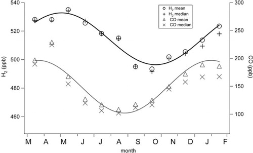
We observed a pronounced seasonal cycle of H₂ (Fig. 4) displaying a maximum in late winter/early spring and a minimum in late summer/early autumn. Such seasonal variation has previously been attributed to maximal summertime loss rates by the OH radical combined with the strongest rates of soil deposition for drier soil conditions (e.g. Novelli et al., 1999; Barnes et al., 2003b; Steinbacher et al., 2007; Lallo et al., 2008). The 2-month lag in the H₂ minimum relative to CO is a result of the soil sink which becomes more dominant later in the year when optimum soil moisture levels occur. Several field and laboratory studies have highlighted the importance of soil moisture on the deposition of H₂, broadly showing decreased deposition with increased moisture content (e.g. Conrad and Seiler, 1981; Yonemura et al., 1999, 2000; Smith-Downey et al., 2006). The seasonal cycle can be described with a sinusoidal fit with a peak to trough magnitude of approximately 40 ppb in close agreement with other studies for this latitudinal range (Novelli et al., 1999; Simmonds et al., 2000; Barnes et al., 2003b; Steinbacher et al., 2007; Grant et al., 2010b). It is notable that the minimum monthly value was in October, whereas the largest number of nocturnal deposition events occur between May and August. This is likely due to the localised nature of night-time depletion, which also depends on the formation of a nocturnal boundary layer (nBL) with reduced surface mixing, and may have been favoured at that time of year. The monthly average values, in contrast, may be more influenced by soil conditions over a wider geographic area and represent both day- and night-time conditions.

Fig. 4.  Monthly means and medians of H₂ and CO at Weybourne. The lines represent sine wave fits to the mean values.

3.3. Diurnal cycle of H₂

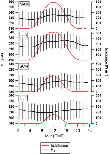
We investigated the diurnal cycle of H₂ mixing ratios at Weybourne by calculating a daily hourly mean and further grouping this in 3-month periods, namely March, April and May (MAM); June, July and August (JJA); September, October and November (SON), December January and February (DJF) (Fig. 5). There was no evidence of cyclical diel behaviour associated with peak traffic flow in neighbouring towns. Negative excursions were apparent for MAM, JJA and SON with lower mixing ratios and larger standard deviations at night and early morning most likely due to the uptake by soils within a contained nBL or shallow inversion. The day-night differences in summer months may also have been augmented by daytime photochemical formation of H₂ in polluted air masses. We speculate that the daily cycle at Weybourne was largely governed by the mixing of air from the nBL with that from the residual layer as vertical mixing increased after sunrise. The morning rise in H₂ was consistent with the time of sunrise during these three periods, i.e. later in SON than JJA.

Fig. 5.  Hourly means for H₂ mixing ratio and hourly means for irradiance at Weybourne for MAM, JJA, SON and DJF. Error bars represent±one sigma standard deviation of the hourly mean H₂ mixing ratio.

3.4. ΔH₂ by wind sector

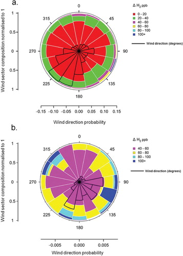
It is evident from Fig. 6a that the prominent wind direction during the study period was SW–SSW and approximately 54% of H₂ measurements were made in air coming from this direction. The same panel shows that over 95% of the time the ΔH₂ was below 40 ppb for all of the wind sectors. There is little evidence of any wind direction dependency in panel a, and this only becomes apparent when the data are filtered to remove ΔH₂<40 ppb (panel b). This latter panel represents just 3.5% (1275 data points) of the data displayed in panel a. The highest ΔH₂ values (i.e. in the categories 80–100 ppb and> 100 ppb) were a feature of wind directions between SSW and E, consistent with transport of polluted air from the London region and in outflow from northern Europe, respectively. This range of wind directions encompasses~70% of all wind directions associated with the filtered data set. Maximum ΔH₂ values were associated with winds from the ESE and were dominated by a single event on the 5 February 2009 (see Section 3.6). On a small number of occasions (<1.5% of the data included in panel b), ΔH₂ values above 100 ppb were observed in air from the WNW–NW (Fig. 1) in the direction of the major centres of H₂ production in the UK.

Fig. 6.  Wind rose showing the distribution of ΔH₂ for (a) all positive ΔH₂ and (b) data above a ΔH₂ of 40 ppb. Radial axis represents probability and the legends show mixing ratio ranges colour coded. A wind rose showing the wind distribution is shown on each panel in black.

3.5. ΔH₂/ΔCO in polluted air

As H₂ and CO share common sources and sinks, information may be gained by examining the ratio of H₂ to CO in air arriving at Weybourne. As both H₂ and CO have strong seasonal cycles that are out of phase with one another (Fig. 4), it was important to first remove this seasonality by subtracting the seasonally varying background or baseline concentrations before calculating a ratio of ‘excess’ H₂ to ‘excess’ CO (i.e. ΔH₂/ΔCO, mole H₂/mole CO; see Barnes et al., 2003b; Grant et al., 2010a; Bond et al., 2011). The influence of the adopted methodology for subtracting background H₂ and CO (Section 3.1) on the resulting slope of correlations between ΔH₂ and ΔCO was tested for quantile probabilities of 0.1 to 0.3 and 0.02 to 0.1 for H₂ and CO, respectively. The variation in the resulting slopes of ΔH₂ versus ΔCO showed less than 5% variation between all permutations and was well within the uncertainty of the respective regressions.

Previous studies at the remote monitoring stations at Mace Head, Ireland and Jungfraujoch, Switzerland report ΔH₂/ΔCO mole ratios of 0.15–0.18 (Simmonds et al., 2000; Grant et al., 2010b) and 0.26–0.32 (Bond et al., 2011), respectively. Such values are consistently lower than those reported in urban and suburban areas where ΔH₂/ΔCO ratios have been reported in the range 0.4–0.53 for rush hour traffic (e.g. Steinbacher et al., 2007; Aalto et al., 2009; Hammer et al., 2009; Yver et al., 2009; Grant et al., 2010a) and from direct source studies investigating traffic emissions performed in the Heidelberg/Mannheim region, Germany, where mean ΔH₂/ΔCO ratios were 0.45±0.07 (Hammer et al., 2009). In addition, a ΔH₂/ΔCO of 0.48±0.12 was measured in a highway tunnel study in Zurich, Switzerland (Vollmer et al., 2007).

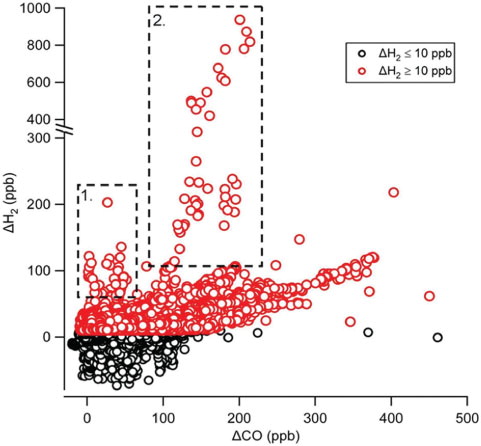
Figure 7 shows ΔH₂ versus ΔCO for all data. A number of features are evident in this figure. The large numbers of negative ΔH₂ values reflect the propensity for H₂ to be subject to depositional loss, whereas significantly negative ΔCO values were rare and small in magnitude. On a few occasions, very large excursions in ΔH₂ were observed, which we attribute to specific sources in Section 3.6. Reduced major axis regression analysis (note: all data inside boxes 1 and 2 in Fig. 7 were excluded from all regression analyses in this section) yielded a slope of 0.35±0.002 with a low correlation coefficient (r²=0.25) for all remaining ΔH₂/ΔCO data. To avoid episodes of high H₂ deposition during periods of strong inversions and low wind speeds, and also to avoid errors in subtracting backgrounds at low values of ΔH₂, the data were filtered to exclude ΔH₂ values below + 10 ppb. This yields a slope of 0.25±0.002 with a marginally improved correlation coefficient (r²=0.32).

Fig. 7.  ΔH₂ vs. ΔCO for all data collected between March 2008 and February 2009. Dashed boxes labelled 1 and 2 correspond to event 1 and event 2 in Section 3.6, respectively. Note the change in scale on y-axis above 300 ppb H₂.

To further disaggregate the data and to investigate possible seasonal differences in ΔH₂/ΔCO, the measurements were grouped in to 3-month blocks (Fig. 8). In an attempt to also target the more polluted conditions, we also used NO_x measurements as an additional filtering criterion, removing those data with NO_x mixing ratios below 5 ppb. Both sets of filtered data are shown in Fig. 8. Measurements from the high H₂ events shown in the boxes in Fig. 7 were also excluded. Some events of high H₂ and relatively low CO persist in this figure and in most (but not all) cases were generally associated with lower pollution (NO_x) abundance. Again we interpret these as being due to non-vehicular emissions, and those with higher NO_x may simply have been subject to mixture with more generally polluted air encountered along the air mass trajectory. Industrial emissions of H₂ may or may not be associated with CO. For instance, steam or thermal reforming of natural gas produces a mixture of H₂ and CO (syngas) and could give rise to events with covarying H₂ and CO. Most high H₂ events, however, appeared to be largely independent of CO abundance.

Fig. 8.  ΔH₂ vs. ΔCO in each of four seasons for elevated ΔH₂ (≥10 ppb) and also filtered for polluted conditions (NO_x>5 ppb). ΔH₂ values above 150 ppb have been excluded as these belong almost exclusively to the periods of anomalously high H₂ (i.e. corresponding to boxes 1 and 2 in Fig. 7). Regression analysis was performed for the data where NO_x was above 5 ppb NO_x. The dashed lines in each panel represent ΔH₂/ΔCO ratios of approximately 0.36 to 0.6, which are representative of near-source vehicle emission ratios reported in the literature (see text in Section 3.5).

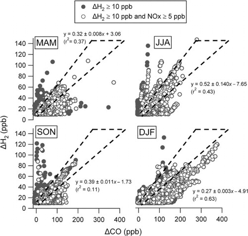
The dashed envelopes in Fig. 8 mark the range of ratios reported close to vehicle emissions as reviewed above, i.e. 0.36–0.60. The seasonally divided data suggest somewhat greater correlations in some seasons than others, largely as a result of specific events: e.g. note the sustained event with a compact correlation observed during the DJF period. In general, the bulk of the data (notably those at high NO_x) fall towards the lower end of these envelopes, which may be indicative of loss of H₂ during transport. There are also apparent ‘clusters’ of highly correlated ΔH₂ and ΔCO values, which we hypothesise as are representative of individual long-range transported urban pollution plumes arriving at Weybourne. There is some evidence that the ratios tend to be lowest in the DJF period and highest in JJA (note the correlation coefficients shown in the figure). This may at first seem counterintuitive given that the seasonal minimum in H₂ occurs in SON, but this may relate to higher photochemical production of H₂ from degradation of hydrocarbons and photolysis of formaldehyde in summer. The DJF period, however, is also characterised by higher ΔCO conditions and so may not be readily comparable to other seasons. For instance, it might be that the winter period is characterised by a different mix of combustion sources (e.g. greater static combustion versus mobile).

We conclude that caution must be applied when using ΔH₂/ΔCO determined from measurements at remote locations as a means of scaling CO emission inventories to estimate H₂ emission inventories, as has been done in some studies, since the ratios measured at the receptor are potentially subject to a number of post-emission processes.

3.6. Extreme H₂ pollution event

Instances where the ΔH₂ versus ΔCO relationships were substantially different from the bulk of the data are highlighted in Fig. 7 using dashed boxes. These events yielded ΔH₂/ΔCO ratios greater than those observed in fresh pollution (see references in Section 3.5). This suggests the existence of an additional H₂ source. This was investigated further by focusing on the two most prominent examples of this, namely 4 to 7 a.m. (GMT) on the 5 July 2008 and 0 to 3 a.m. on the 5 February 2009, which were called event 1 and event 2, respectively. The maximum H₂ during event 1 was 602 ppb, with a mean ΔH₂/ΔCO of 1.92±0.54. In event 2, a much higher maximum H₂ mixing ratio was measured at 1450 ppb coincident with a maximum CO mixing ratio of 366 ppb. The mean ΔH₂/ΔCO during event 2 was 2.6±1.3. Both events occurred at night and under low wind speeds, thus minimising mixing of any plume from a point source, as both events appear to be due to.

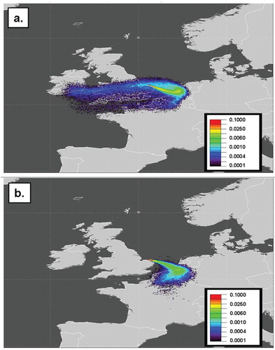
NAME footprints were employed to investigate the possible origins of high H₂ during these events (Fig. 9), and it was apparent that air-masses arriving at Weybourne during these periods had been subject to considerable surface exposure (below 100 m altitude) in the Benelux region. Maisonnier and Perrin (2007) report that 15.8×10⁹ m³ a⁻¹ of H₂ is produced in Netherlands and Belgium combined, amounting to 18% of total European production. Production facilities in Antwerp, Belgium and Zeeland, Netherlands alone produce 3.9 × 10⁹ m³ a⁻¹ and 4.2×10⁹ m³ a⁻¹, respectively. However, it must be noted that the report highlighted 10 large H₂ production facilities in Benelux, and other point sources, may exist, so it is not possible to identify a specific origin.

Fig. 9.  NAME back-maps showing surface exposure (0–100 m) for air arriving at Weybourne between (a) 06:00 and 09:00 on the 5 July 2008 and (b) 03:00 and 06:00 on the 5 February 2009. The percentage of total air mass is the fraction of the 30 000 particles released that are detected in each 0.05°×0.05° grid box during the 2 d prior to the release.

3.7. Estimation of H₂ deposition velocity

The main sink in the atmospheric molecular H₂ cycle is the uptake by soils, which is thought to account for the removal of between 55 and 88 Tg a⁻¹ (Novelli et al., 1999; Hauglustaine and Ehhalt, 2002; Sanderson et al., 2003; Rhee et al., 2006; Price et al., 2007; Xiao et al., 2007; Ehhalt and Rohrer, 2009; Pieterse et al., 2011; Yashiro et al., 2011). The mechanisms controlling H₂ uptake by soils remain poorly understood, but the majority of studies suggest that it is mediated by abiontic soil enzymes (e.g. Conrad et al., 1983; Conrad, 1996). However, this view has recently been challenged by Constant et al. (2010) who propose that specialised H₂-oxidizing actinobacteria are responsible.

Previous studies have estimated the deposition velocity of H₂ to the soil using a range of techniques. Flux chambers have been utilised both in the field and in the laboratory and have the advantage that they can be used to investigate a broad range of soil types and environments with a relatively high degree of control. Such studies have been critical in highlighting some potential environmental factors controlling the deposition of H₂ to the soil including soil moisture (e.g. Conrad and Seiler, 1985; Yonemura et al., 1999, 2000; Lallo et al., 2008; Schmitt et al., 2009) and temperature (e.g. Liebl and Seiler, 1976; Trevors, 1985; Lallo et al., 2008). H₂ deposition velocity can also be determined ‘top-down’ using atmospheric measurements. These latter studies have utilised a range of techniques and atmospheric measurements to estimate the deposition velocity of H₂ including the ozone box method (Simmonds et al., 2000, 2011), the radon tracer method (Hammer and Lallo et al., 2009; Levin, 2009; Yver et al., 2009), concentration gradients (Rahn et al., 2002; Constant et al., 2008) and nocturnal decay of H₂ (Steinbacher et al., 2007). Some estimates from the “top-down” approach are displayed in Table 1.

In this study, the deposition velocity of H₂ was investigated using atmospheric measurements of H₂ and O₃ when strong depletions in H₂ and O₃ were coincident with a shallow nBL (after Simmonds et al., 2000). The decrease in O₃ was used to estimate the height of the inversion assuming a constant deposition velocity for O₃. As the deposition velocity of O₃ is well quantified from other studies, we used this to estimate the height of the nBL using1

where v _d (m s⁻¹) is the deposition velocity, h the nBL height in metres and k ₁ is the first order decay constant (s⁻¹) of O₃ derived from direct observations using2

where X is the mole fraction of the depositing species (i.e. O₃), t is time after the beginning of the deposition event in seconds, [X] _t is the mole fraction at time t and [X]₀ is the mole fraction at the start of the event.

An O₃ deposition velocity of 2.5×10⁻³ m s⁻¹ was used in this study to derive the nBL height. For consistency, we use O₃ deposition velocities from the same study as that used by Simmonds et al. (2000). This study took place at Auchencorth Moss in the Scottish Borders where nocturnal summertime/autumn O₃ dry deposition velocities were measured in the range 2 to 3×10⁻³ m s⁻¹ (Photochemical Oxidant Review Group, 1997).

As this approach relied on O₃ deposition, a strict set of selection criteria were chosen in order to select events for further analysis. An event was considered suitable if the conditions met with the following criteria: (1) nights when a decrease in H₂ was strongly associated with a decrease in O₃; (2) low pollution, particularly low NO below 1 ppb to limit the possible effects of chemistry on observed ozone; (3) consistent SW-SE flow such that air arriving at the site had been predominantly moving over land; and (4) a strong nocturnal inversion as diagnosed using the SODAR-RASS.

The periods selected for further study were 11–17 June 2008 and the 25–30 July 2008. The relevant chemistry and meteorology for the chosen events is shown in Fig. 10a and b and the vertical potential temperature profiles for the periods are shown in Fig. 11a and b. The blue transparent rectangles in Fig. 10 show the specific time periods chosen.

Fig. 10.  H₂ deposition events used to estimate H₂ deposition velocity for (a) 11–17 June 2008 and (b) 25–30 July 2008. Events used are highlighted using blue transparent rectangles.

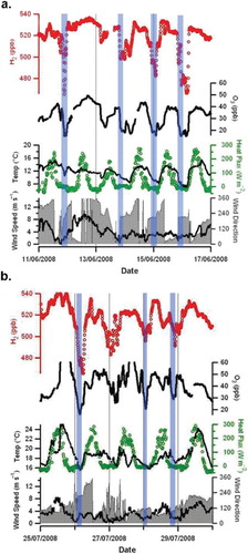
Fig. 11.  RASS potential temperature for the H₂ deposition events used to estimate H₂ deposition velocity for (a) 11–17 June 2008 and (b) 25–30 July 2008. Black circles represent the nBL heights estimated from O₃ deposition in Section 3.7 and corresponding to the blue transparent rectangles shown in Fig. 10.

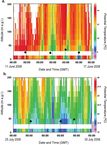
The thermal stratification of the nBL was stable throughout all the nights in these two periods. In Fig. 11a, green colours below orange and red colours indicate cool surface air underneath warmer air in the residual layer above. The depth of this cool nBL was between 50 and100 m, exhibiting its maximum depth in the nights between June 13 and 14. In Fig. 11b, colours gradually change with height indicating that the nBL was stable throughout with temperature increasing steadily with height. This situation could be termed as a surface inversion. Inversion heights probably ranged from a few metres to a few tens of metres, although this cannot be proved directly from the RASS data, because the lowest measurement height was 30 m. However, the inversion height analysis is supported by the nocturnal wind speed minima and vertical heat flux depicted in Fig. 10.

Measured O₃ decay rates were in the range 0.49×10⁻⁴ s⁻¹ to 1.34 × 10⁻⁴ s⁻¹, giving nBL height estimates in he range 18 to 50 m for the two periods investigated. The nBL height estimated for each event using the ozone box methods is depicted in Fig. 11a and b. This height range is supported by the analysis of Fig. 11. Decay constants for H₂ were in the range 0.27×10⁻⁵ s⁻¹ to 1.83×10⁻⁵ s⁻¹ with corresponding H₂ deposition velocities in the range 2.7×10⁻⁴ m s⁻¹ to 4.4×10⁻⁴ m s⁻¹ and 1.3×10⁻⁴ m s⁻¹ to 3.2×10⁻⁴ m s⁻¹ for June and July 2008, respectively. These estimates are in reasonable agreement with previous studies using the top-down approach where estimates range from 0.18 to 12.9×10⁻⁴ m s⁻¹ (Table 1). However, it must be noted that the deposition estimates tabulated in Table 1 are derived from a range of soil types. The soil type at Weybourne and the surrounding area is best described as fine loamy sand (Corbett and Tatler, 1974).

Table 1. Comparison of H₂ deposition velocity estimates using a ‘top-down’ approach

Environment	H2 deposition velocity (×10^−4 m s^−1)	Method	Citation
Boreal forest	7.3±1.5 (0.9–5.6)	Concentration gradients	Rahn et al. (2002)
Urban	0.5–1^a	Nocturnal H2 decay	Steinbacher et al. (2007)
Rural	1.5 (0–0.33)	Concentration gradients	Constant et al. (2008)
Urban	3±0.7 (2.3–3.7)	Radon tracer	Hammer and Levin (2009)
Urban	2.4±1.3 (0–5.1)	Radon tracer	Yver et al. (2009)
Urban	2.2 (0.9–5.7)	Nocturnal H2 depletion and calculated BL heights	Grant et al. (2010a)
Rural/coastal	2.6^b	Ozone box	Simmonds et al. (2000)
	5.3±1.6 (1.8–12.9)	Ozone box	Simmonds et al. (2011)
Urban	1.3–7^a	Radon tracer	Lallo et al. (2009)
Rural/coastal	3.5±0.7 (2.7–4.4) (June 2008)	Ozone box	This work
	1.9±1 (1.3–3.2) (July 2008)

^aNo mean value reported.

^bNo range reported.

3.8. Arctic and maritime air masses

Between 13 and 21 May 2008, Weybourne encountered a prolonged period of northerly flow during which the stability of H₂, CO, O₃ and NO_x (Fig. 12) suggested that the air sampled had received little influence from regional local pollution sources. NAME air mass footprints showed that the dominant air mass during this period was from Northern Scandinavia and Arctic regions briefly interrupted by air which appeared to have been subject to long-range maritime transport (Fig. 13).

Fig. 12.  H₂, CO, O₃, NO, NO₂ and wind direction for the period of strong northerly flow observed during May 2008. The dashed lines numbered 1–4 correspond to number air-mass trajectory maps numbered 1–4 shown in Fig. 13.

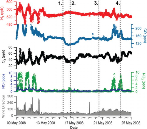
Fig. 13.  Ten-day NAME back-maps showing the probability of surface influence (0–1000 m) for 12:00–14:00 h for 15 May 2008 (top left), 16 May 2008 (top right), 20 May 2008 (bottom left) and 23 May 2008 (bottom right).

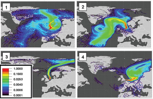
The mean H₂ mixing ratio during the Arctic flow (e.g. event marker 1 in Fig. 12) was 532±4.5 ppb making this by far the least variable period during the study. In addition very little variation in the CO (147±4 ppb) and O₃ (51±4 ppb) was measured. From dawn on the 15 May 2008 until noon on the 17 May 2008, a change in air mass was apparent with a slight increase in the H₂ mixing ratio to a mean of 541 ppb between about midnight on the 16 May until noon on the 17 May (event marker 2). Coincident with this was a distinct decrease in both CO and O₃ with means of 121 ppb and 39 ppb, respectively. This is consistent with a source from lower latitudes as the increase in H₂ mixing ratios with lower latitudes in the Northern Hemisphere is well documented (Novelli et al., 1999; Price et al., 2007). Model simulations by Price et al. (2007) highlight the strong year round photochemical source of H₂ within the tropical regions as compared with the seasonal variation observed at higher latitudes. In contrast, CO shows increasing mixing ratios with increasing latitude in the Northern Hemisphere (Novelli, 2003). For Mace Head, Ireland, it has previously been shown that low O₃ and CO can be attributed to long-range transport events involving ‘tropical maritime’ air masses from the North Atlantic region below 40°S (Derwent et al., 1998). Further to this, Simmonds et al. (2000) noted that such events have corresponding high H₂ mixing ratios and also attribute this to long-range transport of air masses from the tropical North Atlantic. NAME air mass footprints (e.g. event marker 2 in Figs. 12 and 13) for the period between 15 May until noon on the 17 May do indeed indicate anticyclonic transport of air from the subtropical Atlantic first northwards to Iceland and then south across the length of the North Sea to Weybourne, with no passage over land.

By the time of event marker 3, the air flow, while still strongly northerly, no longer originated in the subtropics, but rather from the Arctic, and H₂, CO and O₃ had returned to the same mixing ratios as before the ‘subtropical’ interlude. As the air stream turned more towards the east (event marker 4), increasing amounts of pollution originating in Northern Europe began to influence CO, H₂ and ozone abundances once more.

4. Conclusions

We have reported the first continuous measurements of atmospheric H₂ in the UK, from a rural location that is predominantly impacted by moderately polluted air masses emanating from urban and industrial areas in Britain and the near-continent. Some similar phenomena to those observed at other rural and regional sites, such as the longer-running and largely marine-influenced Mace Head observatory in Eire, were noted. The same background seasonal cycle was seen as has been reported at Mace Head, albeit with larger and more frequent positive excursions due to entrainment of polluted air and, at certain times of year, frequent negative events were evidently associated with loss of H₂ to soil during conditions of limited vertical mixing. We also noted a rare occurrence of flow from the subtropical Atlantic with low CO and slightly elevated H₂ characteristic of pristine tropical marine air. Taken together, these observations emphasise the sensitivity of atmospheric H₂ to uptake by soils.

A particular novelty of this study was the observation of events with exceptionally high H₂ levels, for which the ratios of ‘excess’ (i.e. above background) H₂ to CO (ΔH₂/ΔCO) were far higher than could be explained by emissions from the transport sector, suggesting additional industrial sources; evidently located in regions of Benelux and NE England. A knowledge of H₂/CO emission ratios from different industrial sources may allow discrimination of different processes, e.g. steam reforming of natural gas versus by-product release from chemical manufacturing, which should differ substantially in such ratios.

We have also demonstrated that deposition velocities of H₂ can be calculated by observing decay rates during episodes of slack winds and intense nBL formation. The estimates are improved by knowledge of the actual boundary layer height, and we suggest that more frequent and more accurate measurements, independent of assumed ozone deposition rates, might be achieved by improvements to the resolution and range of the instrumentation used for the vertical soundings.

The final conclusion of the study is that scaling of CO measurements to estimate H₂ emissions should be approached with substantial caution since (a) H₂/CO emission ratios may differ substantially between sources and (b) H₂/CO ratios may be substantially modified during transport to a receptor site either by in situ photochemical production or by deposition to soils at rates that vary both with season (soil moisture and temperature) and with local meteorology. Detailed trajectory modelling incorporating atmospheric chemistry and deposition rates would be required to deconvolve these processes.

We believe that the approach taken of making frequent and continuous high precision measurements of H₂ and CO, along with complementary meteorological and chemical measurements, provides additional insight in to the origins and processes affecting atmospheric molecular hydrogen.

Acknowledgements

This work was funded by the EU Framework 6 project EuroHydros (A European Network for Atmospheric Hydrogen observations and studies; GOCE 036916). We would like to thank the National Centre for Atmospheric Sciences (NCAS), which support the Weybourne Atmospheric Observatory through the Facility for Ground based Atmospheric Measurements (FGAM). We would like to thank the Met office for use of the NAME model and Alistair Manning for guidance in its use.

References

- Aalto T, Lallo M, Hatakka J, Laurila T. Atmospheric hydrogen variations and traffic emissions at an urban site in Finland. Atmos. Chem. Phys. 2009; 9: 7387–7396. 10.3402/tellusb.v64i0.17771.
- Barnes, D. H, Wofsy, S. C, Fehlau, B. P, Gottlieb, E. W, Elkins, J. W. and co-authors. 2003a. Urban/industrial pollution for the New York City–Washington, D. C., corridor, 1996–1998: 1. Providing independent verification of CO and PCE emissions inventories. J. Geophys. Res. 108(D6): 4185–4196. 10.3402/tellusb.v64i0.17771.
- Barnes, D. H, Wofsy, S. C, Fehlau, B. P, Gottlieb, E. W, Elkins, J. W. and co-authors. 2003b. Hydrogen in the atmosphere: observations above a forest canopy in a polluted environment. J. Geophys. Res. 108(D6): 4197–4206. 10.3402/tellusb.v64i0.17771.
- Bond S. W, Vollmer M. K, Steinbacher M, Henne S, Reimann S. Atmospheric molecular hydrogen (H2): observations at the high-altitude site Jungfraujoch, Switzerland. Tellus. 2011; 63B(1): 64–76.
- Conrad R. Soil microorganisms as controllers of atmospheric trace gases (H2, CO, CH4, OCS, N2O, and NO). Microbiol. Rev. 1996; 60(4): 609–640.
- Conrad R, Seiler W. Decomposition of atmospheric hydrogen by soil microorganisms and soil enzymes. Soil Biol. Biochem. 1981; 13(1): 43–49. 10.3402/tellusb.v64i0.17771.
- Conrad R, Seiler W. Influence of temperature, moisture, and organic carbon on the flux of H2 and CO between soil and atmosphere: field studies in subtropical regions. J. Geophys. Res. 1985; 90(D3): 5699–5709. 10.3402/tellusb.v64i0.17771.
- Conrad R, Weber M, Seiler W. Kinetics and electron transport of soil hydrogenases catalyzing the oxidation of atmospheric hydrogen. Soil. Biol. Biochem. 1983; 15(2): 167–173. 10.3402/tellusb.v64i0.17771.
- Constant P, Chowdhury S. P, Pratscher J, Conrad R. Streptomycetes contributing to atmospheric molecular hydrogen soil uptake are widespread and encode a putative high-affinity [NiFe]-hydrogenase. Environ. Microbiol. 2010; 12(3): 821–829. 10.3402/tellusb.v64i0.17771.
- Constant P, Poissant L, Villemur R. Annual hydrogen, carbon monoxide and carbon dioxide concentrations and surface to air exchanges in a rural area (Québec, Canada). Atmos. Environ. 2008; 42(20): 5090–5100. 10.3402/tellusb.v64i0.17771.
- Corbett, W. M and Tatler, W. 1974. Soils in Norfolk II: Sheets TG 13/14 (Barningham/Sheringham). Soil Survey Record No. 21. Adlord & Sons Ltd, Bartholomew Press: DorkingUK.
- Derwent, R. G, Simmonds, P. G, O'Doherty, S, Manning, A. J, Collins, W. and co-authors. 2006. Global environmental impacts of the hydrogen economy. Int. J. Nucl. Hydrogen Prod. Appl. 1(1): 57–67. 10.3402/tellusb.v64i0.17771.
- Derwent R. G, Simmonds P. G, Seuring S, Dimmer C. Observation and interpretation of the seasonal cycles in the surface concentrations of ozone and carbon monoxide at mace head, Ireland from 1990 to 1994. Atmos. Environ. 1998; 32(2): 145–157. 10.3402/tellusb.v64i0.17771.
- Ehhalt D. H, Rohrer F. The tropospheric cycle of H2: a critical review. Tellus. 2009; 61B(3): 500–535.
- Emeis S, Schäfer K, Münkel C. Surface-based remote sensing of the mixing-layer height – a review. Meteorol. Z. 2008; 17(5): 621–630. 10.3402/tellusb.v64i0.17771.
- Fleming Z. L, Monks P. S, Manning A. J. Review: untangling the influence of air-mass history in interpreting observed atmospheric composition. Atmos. Res. 2012; 104–105: 1–39. 10.3402/tellusb.v64i0.17771.
- Grant A, Stanley K. F, Henshaw S. J, Shallcross D. E, O'Doherty S. High-frequency urban measurements of molecular hydrogen and carbon monoxide in the United Kingdom. Atmos. Chem. Phys. 2010a; 10(10): 4715–4724. 10.3402/tellusb.v64i0.17771.
- Grant A, Witham C. S, Simmonds P. G, Manning A. J, O'Doherty S. A 15 year record of high-frequency, in situ measurements of hydrogen at Mace Head, Ireland. Atmos. Chem. Phys. 2010b; 10(3): 1203–1214. 10.3402/tellusb.v64i0.17771.
- Hammer S, Levin I. Seasonal variation of the molecular hydrogen uptake by soils inferred from continuous atmospheric observations in Heidelberg, southwest Germany. Tellus. 2009; 61B(3): 556–565.
- Hammer S, Vogel F, Kaul M, Levin I. The H2/CO ratio of emissions from combustion sources: comparison of top-down with bottom-up measurements in southwest Germany. Tellus. 2009; 61B(3): 547–555.
- Hauglustaine D. A, Ehhalt D. H. A three-dimensional model of molecular hydrogen in the troposphere. J. Geophys. Res. 2002; 107(D17): 1–16. 10.3402/tellusb.v64i0.17771.
- Jordan A, Steinberg B. Calibration of atmospheric hydrogen measurements. Atmos. Meas. Technol. 2011; 4(3): 509–521. 10.3402/tellusb.v64i0.17771.
- Khalil M. A. K, Rasmussen R. A. Global increase of atmospheric molecular hydrogen. Nature. 1990; 347: 734–745. 10.3402/tellusb.v64i0.17771.
- Lallo M, Aalto T, Laurila T, Hatakka J. Seasonal variations in hydrogen deposition to boreal forest soil in southern Finland. Geophys. Res. Lett. 2008; 35(4): 1–4. 10.3402/tellusb.v64i0.17771.
- Lallo M, Aalto T, Hatakka J, Laurila T. Hydrogen soil de- position at an urban site in Finland. 2009; 5: 8559–8571. 10.3402/tellusb.v64i0.17771.
- Liebl K, Seiler W. CO2 and H2 destruction at the soil surface in production and utilization of gases. Microbial Production and Utilization of Gases. Schlegel H. G.Gottschalk G.Pfenning N.E. Goltze, Göttingen: Germany, 1976; 215–229.
- Manning, A, Jordan, A, Levin, I, Schmidt, M, Neubert, R. E. M. and co-authors. 2009. Final report on CarboEurope “Cucumbers” intercomparison programme. 2009. Online at: http://cucumbers.uea.ac.uk..
- Maisonnier, G and Perrin, J. 2007. Roads2HyCom. European Hydrogen Infrastructure Atlas. Part 2. Industrial surplus hydrogen and markets and production. Document number R2H2006PU.1. (eds. R. Steinberger-Wickens and S. C. Trumper). PLANET GbR, Oldenberg, Germany. Online at: http://www.roads2hy.com..
- Novelli P. C. Reanalysis of tropospheric CO trends: effects of the 1997–1998 wildfires. J. Geophys. Res. 2003; 108(D15): 4464.10.3402/tellusb.v64i0.17771.
- Novelli, P. C, Lang, P. M, Masarie, K. A, Hurst, D. F, Elkins, J. W. and co-authors. 1999. Molecular hydrogen in the troposphere: global distribution and budget. J. Atmos. Chem. 104(D23): 30427–30444. 10.3402/tellusb.v64i0.17771.
- Penkett S. A, Plane J. M. C, Comes F. J, Clemitshaw K. C. The Weybourne Atmospheric Observatory. 1999; 2(2): 107–110. 10.3402/tellusb.v64i0.17771.
- Photochemical Oxidant Review Group (PORG). 1997. Ozone in the United Kingdom. Fourth Report. Department of the Environment: London.
- Pieterse, G, Krol, M. C, Batenburg, A. M, Steele, L. P, Krummel, P. B. and co-authors. 2011. Global modelling of H2 mixing ratios and isotopic compositions with the TM5 model. J. Geophys. Res. 11: 7001–7026. 10.3402/tellusb.v64i0.17771.
- Price, H, Jaeglé, L, Rice, A, Quay, P, Novelli, P. C. and co-authors. 2007. Global budget of molecular hydrogen and its deuterium content: constraints from ground station, cruise, and aircraft observations. Geophys. Res. Lett. 112(D22): 1–16. 10.3402/tellusb.v64i0.17771.
- Rahn T, Eiler J. M, Kitchen N, Fessenden J. E, Randerson J. T. Concentration and δD of molecular hydrogen in boreal forests: ecosystem-scale systematics of atmospheric H2. Atmos. Chem. Phys. 2002; 29(18): 10–13. 10.3402/tellusb.v64i0.17771.
- Rhee T. S, Brenninkmeijer C. A. M, Röckmann T. The overwhelming role of soils in the global atmospheric hydrogen cycle. Atmos. Environ. 2006; 6: 1611–1625. 10.3402/tellusb.v64i0.17771.
- Ryall D. B, Derwent R. G, Manning A. J, Simmonds P. G, O'Doherty S. Estimating source regions of European emissions of trace gases from observations at Mace Head. J. Atmos. Chem. 2001; 35(14): 2507–2523. 10.3402/tellusb.v64i0.17771.
- Sanderson M. G, Collins W. J, Derwent R. G, Johnson C. E. Simulation of global hydrogen levels using a Lagrangian three dimensional model. Tellus. 2003; 46: 15–28. 10.3402/tellusb.v64i0.17771.
- Schmitt S, Hanselmann A, Wollschläger U, Hammer S, Levin I. Investigation of parameters controlling the soil sink of atmospheric molecular hydrogen. Science. 2009; 61B(2): 416–423.
- Schultz M. G, Diehl T, Brasseur G. P, Zittel W. Air pollution and climate-forcing impacts of a global hydrogen economy. Tellus. 2003; 302(5645): 624–627. 10.3402/tellusb.v64i0.17771.
- Simmonds, P. G, Derwent, R. G, Manning, A. J, Grant, A, O'Doherty, S. and co-authors. 2011. Estimation of hydrogen deposition velocities from 1995–2008 at Mace Head, Ireland using a simple box model and concurrent ozone depositions. J. Geophys. Res. 63B: 40–51.
- Simmonds, P. G, Derwent, R. G, O'Doherty, S, Ryall, D. B, Steele, L. P. and co-authors. 2000. Continuous high-frequency observations of hydrogen at the Mace Head baseline atmospheric monitoring station over the 1994–1998 period. Geophys. Res. Lett. 105(D10): 12105–12121. 10.3402/tellusb.v64i0.17771.
- Smith-Downey N. V, Randerson J. T, Eiler J. M. Temperature and moisture dependence of soil H2 uptake measured in the laboratory. Atmos. Environ. 2006; 33(L14813): 1–5.
- Steinbacher, M, Fischer, A, Vollmer, M. K, Buchmann, B, Reimann, S. and co-authors. 2007. Perennial observations of molecular hydrogen (H2) at a suburban site in Switzerland. Plant Soil. 41(10): 2111–2124. 10.3402/tellusb.v64i0.17771.
- Trevors J. T. Hydrogen consumption in soil. Science. 1985; 87: 417–422. 10.3402/tellusb.v64i0.17771.
- Tromp T. K, Shia R.-L, Allen M, Eiler J. M, Yung Y. L. Potential environmental impact of a hydrogen economy on the stratosphere. Atmos. Environ. 2003; 300(5626): 1740–2174. 10.3402/tellusb.v64i0.17771.
- Vollmer, M. K, Juergens, N, Steinbacher, M, Reimann, S, Weilenmann, M. and co-authors. 2007. Road vehicle emissions of molecular hydrogen (H2) from a tunnel study. Geophys. Res. Lett. 41(37): 8355–8369. 10.3402/tellusb.v64i0.17771.
- Warwick N. J, Bekki S, Nisbet E. G, Pyle J. A. Impact of a hydrogen economy on the stratosphere and troposphere studied in a 2-D model. J. Geophys. Res. 2004; 31(L05107): 1–4.
- Xiao, X, Prinn, R. G, Simmonds, P. G, Steele, L. P, Novelli, P. C. and co-authors. 2007. Optimal estimation of the soil uptake rate of molecular hydrogen from the Advanced Global Atmospheric Gases Experiment and other measurements. Atmos. Chem. Phys. 112(D07303): 1–15.
- Yashiro H, Sudo K, Yonemura S, Takigawa M. The impact of soil uptake on the global distribution of molecular hydrogen: chemical transport model simulation. Tellus. 2011; 11: 6701–6719. 10.3402/tellusb.v64i0.17771.
- Yonemura S, Kawashima S, Tsuruta H. Continuous measurements of CO and H2 deposition velocities onto an andisol: uptake control by soil moisture. Atmos. Environ. 1999; 51B: 688–700.
- Yonemura S, Miyata A, Yokozawa M. Concentrations of carbon monoxide and methane at two heights above a grass field and their deposition onto the field. Atmos. Chem. Phys. 2000; 34(29–30): 5007–5014. 10.3402/tellusb.v64i0.17771.
- Yver, C. E, Pison, I. C, Fortems-Cheiney, A, Schmidt, M, Chevallier, F. and co-authors. 2011. A new estimation of the recent tropospheric molecular hydrogen budget using atmospheric observations and variational inversion. J. Geophys. Res. 11(7): 3375–3392. 10.3402/tellusb.v64i0.17771.
- Yver C. E, Schmidt M, Bousquet P, Zahorowski W, Ramonet M. Estimation of the molecular hydrogen soil uptake and traffic emissions at a suburban site near Paris through hydrogen, carbon monoxide, and radon-222 semicontinuous measurements. Atmos. Chem. Phys. 2009; 114(D18): 1–12. 10.3402/tellusb.v64i0.17771.