What is the climate system able to do ‘on its own’?

ABSTRACT

The climate of the Earth, like planetary climates in general, is broadly controlled by solar irradiation, planetary albedo and emissivity as well as its rotation rate and distribution of land (with its orography) and oceans. However, the majority of climate fluctuations that affect mankind are internal modes of the general circulation of the atmosphere and the oceans. Some of these modes, such as El Niño-Southern Oscillation (ENSO), are quasi-regular and have some longer-term predictive skill; others like the Arctic and Antarctic Oscillation are chaotic and generally unpredictable beyond a few weeks. Studies using general circulation models indicate that internal processes dominate the regional climate and that some like ENSO events have even distinct global signatures. This is one of the reasons why it is so difficult to separate internal climate processes from external ones caused, for example, by changes in greenhouse gases and solar irradiation. However, the accumulation of the warmest seasons during the latest two decades is lending strong support to the forcing of the greenhouse gases. As models are getting more comprehensive, they show a gradually broader range of internal processes including those on longer time scales, challenging the interpretation of the causes of past and present climate events further.

This paper is part of a Thematic Cluster in honor of the late Professor Bert Bolin for his outstanding contributions to climate science.

• climate change
• general circulation models
• natural climate variability

1. Introduction

I believe there are two principally different ways to anticipate and understand climate and the processes that determine it. The first of these is the descriptive view of climate that can be traced back as far as to Pythagoras and Aristotle (Sanderson, 1999). With the rapidly enhanced knowledge of the Earth's geography that evolved during the 19th century, the interest in the climate of the Earth increased rapidly both because of economical needs and scientific curiosity. Considerable contributions came from scientists with a broad scientific and cultural interest, such as Alexander von Humboldt. Over a long period of time starting in the late 19th century, the Russian-German meteorologist Wladimir Köppen developed a classification technique of a descriptive global climatology over a long period of time (Köppen, 1884, 1900, 1936). See also Kollek et al. (2006) for a recent contribution. Köppen's approach was to relate the Earth's vegetation zones and its seasonality to local mean monthly temperature and precipitation data. This simple approach was met with considerable success. Köppen's colourful climate atlases were used in geographical teaching all around the world. The descriptive concept of climate in the spirit of Köppen is in fact still dominant among traditional climatologists, geographers and geologists and almost without exception among the general public. The general issue, why different parts of the world have such different climates, was presented as a matter of fact, and in many regions, the significant inter-annual variations in climate were essentially left unexplained.

With this traditional view, climate is strictly regulated by astronomical, geophysical and geographical boundary conditions and can in essence only change when these boundary conditions are changing. This conceptual view of climate therefore implies a tendency or a preference to interpret adverse climate events as a consequence of external influences such as caused by solar irradiation and volcanic eruptions, or similarly as due to changes in the composition of the atmosphere, such as in the greenhouse gases and in aerosol concentrations.

A different approach is to consider climate as a dynamical system and thus simply calculate the climate of the Earth from the governing hydro-dynamical equations with known radiative forcing and boundary conditions (Pfeffer, 1960). Such an approach will not only create possibilities for an understanding of the climate, but also make it possible to incorporate internal dynamical processes in the Earth's system and the essential role these play in the Earth's atmosphere and oceans. This approach is based on the recognition that climate is composed of all possible weather that is sampled over representative periods of time covering several decades. Climate is simply the complete envelop of weather. The fact that internal non-linear processes play an important role can be seen from many phenomena in the atmosphere and the oceans that have periods that differ significantly from the diurnal and annual cycle of the solar forcing. In fact, the majority of weather systems have time scales that bear little resemblance to the diurnal or annual cycle. The most remarkable example here is perhaps the Quasi-Biennal Oscillation (QBO) with a distinct period of approximately 26 months (Lindzen and Holton, 1968; Baldwin et al., 2001). Another example is the approximate 4-yr cycle of ENSO (El Niño-Southern Oscillation) (Philander, 1990). Other internal processes are essentially aperiodic such as the Arctic and the Antarctic circulation. At higher latitudes of the Northern Hemisphere, the inter-annual variability is a dominant factor, and here the difference between a very mild and a very cold winter can be a considerable fraction of the difference between an average summer and an average winter. In parts of northern Europe, it can be more than 60%.

It seems clear that a dynamical understanding of internal processes in the climate system is necessary in order to understand the physical processes of the climate in terms of the assemblage of weather over a representative period of time. The progress in numerical weather prediction and atmospheric modelling from the middle of the last century has made such an approach feasible.

A first attempt to address climate research and prediction as a computational problem in physics took place at the Advanced Study Institute in Princeton in October 1955 organised by John von Neumann and Jules Charney (Pfeffer, 1960). It followed a similar earlier attempt in 1948 to develop a strategy for numerical weather prediction following the construction of the first electronic computer (Charney et al., 1950). It was generally concluded that climate essentially was controlled by external forcing in combination with surface boundary conditions but would nevertheless have to be addressed as an initial value problem using the fundamental set of physical equations including sources and sinks for heat, water and momentum. This is by and large the approach that has been followed in climate research since then and since 1980 under the auspices of the World Climate Research Programme. The methods used today to explore the dynamics of climate are in all essentials similar to what is used in numerical weather prediction.

General Circulation Models, GCMs, are in many ways building on weather forecasting models, but incorporate a more comprehensive approach including model compartments of the oceans and nowadays also special model components for vegetation and land ices as well as the carbon cycle. The present IPCC 5th assessment to be published in 2013 will include climate simulations using interactive vegetation and carbon cycle modelling. GCMs are now main tools for climate research. The enormous development in computing speed and storage facilities has made it possible today to undertake calculations for millennia with models that can resolve the daily weather systems.

A question that is often asked by many, not the least by scientists from other areas of physics and geophysics, is whether it at all is sensible to make climate simulations by models that lose useful predictability after a few weeks, e.g. Lorenz (1982). This is fully correct if we are concerned with a numerical model that is predicting the weather as an initial value problem. However, this is not the main task of a climate simulation. In that case, we are mainly interested in the statistics of the climate and how the statistics of climate might change when external conditions are changing. How does the frequency or amplitude of a manifold of weather events change (and thus the climate) when we alter the concentration of greenhouse gases or solar radiation, or because of changes in atmospheric opacity due to natural or manmade aerosols? It is therefore important that a model used for climate studies should have corresponding capabilities as a model used for weather prediction even if the weather can only be predicted in a statistical sense. This is what Edward Lorenz called ‘predictability of the second kind’. In fact from a societal view, we are more concerned in extreme events such as excessive heat waves, flooding and violent tropical and extra-tropical cyclones as such events often are highly destructive to society. Will a warmer climate include more damaging events? How can this be explored and what methods do we need to clarify whether extreme events are a consequence of the internal dynamics of the climate system or whether they are consequences of external effects? Or perhaps more correctly, how will the probability distribution of specific weather events be changing, if at all?

An even more fundamental issue is whether climate in itself is uniquely determined by a given set of external forcing and boundary conditions. Can climate just change by chance or if not possible within the present climate, can it occur in a climate with a different concentration of greenhouse gases or different solar irradiation? Has this perhaps happened in the past? Some studies suggest that a non-unique climate is presently not feasible or perhaps more correctly that available models have not yet convincingly demonstrated such non-uniqueness. Recent popular climate literature favours the terminology of climate tipping, such as Lenton et al. (2008).

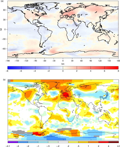
Even if the climate models are imperfect, climate changes studies, such as from increased greenhouse gases, can at first approximation be explored as a contribution of a perturbation on the climate system. We might therefore argue that even if the models have deficiencies, the response of the modelled climate system of such a perturbation, does provide useful insight. Indeed, the results from a large number of climate models suggest that the response to a specified forcing has many characteristic similarities such as the geographical distribution of temperature and precipitation changes. Generally, the pattern of response is proportional to the average amplitude of the forcing but insensitive to the pattern of forcing (Boer and Yu, 2003). Typical changes to a positive perturbation such as increased solar irradiation or increased greenhouse gases manifests itself as a marked warming at high latitudes of the Northern Hemisphere and precipitation increase at high latitudes at both hemispheres. A reversed pattern is generally found for a negative perturbation (Bengtsson, 2001; Kloster et al., 2010). Typical patterns can be seen from Fig. 1, which shows the change of the near-surface temperature during the last 120 yr in steps of 40 yr.

Fig. 1.  Pattern of the near-surface, annual mean temperature trend for the three 40-yr periods, (a) 1890–1930, (b) 1930–1970 and (c) 1970–2010. The global mean temperature trend values are given in Table 1. The large differences of regional trends, in particular, in the Arctic are striking. There is an indication of a positive trend correlation between the tropics and the Arctic, but there is an indication of a negative correlation with high latitudes of the Southern Hemisphere. Equally striking is the superimposed warming during the latest period. (Taken from http://data.giss.nasa.gov/gistemp/maps/)

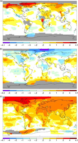
The global mean anomaly values are summarised in Table 1. The total temperature increase has been ca. 0.8°C but most of this has occurred during the last 40 yr. In the period 1930–1970, there was no temperature increase and actually a cooling over land areas and at high latitudes of the Northern Hemisphere. In the first period 1890–1930, on the other hand, there was a minor temperature increase with a warming pattern having some similarities to the warming pattern in the latest period 1970–2010. While the overall warming broadly follows the increase in greenhouse gases, we have no satisfactory explanation to the lack of warming in the intermediate period and solar variability, tropospheric aerosols and natural climate fluctuations have all been suggested. Whilst the first alternative is becoming increasingly unlikely based on solar irradiation observations over the last 35 yr (Fröhlich, 2012), the other two are credible candidates either on their own or in combination. This paper will provide some indications that the last alternative, namely internal climate variations are quite likely to provide variations of this kind. As will be seen such a possibility is suggested from studies of present climate models.

Table 1. Average temperature trend for the three 40-yr periods, 1890–1930, 1930–1970 and 1970–2010

Time period	Near-surface temperature trend/40 yr in °C
1890–1930: Modest tropical warming and distinct Arctic warming, slight cooling over Southern oceans	+0.13
1930–1970: In most aspects a reverse pattern, a marked Arctic cooling	+0.01
1970–2010: A similar pattern as in the period 1890–1930, but a warming trend except for a few limited areas	+0.66

In Section 2, I will comment on typical internal modes of the climate system and the way they manifest themselves in observational records and in model simulation experiments; while in Section 3, I will describe and discuss the implication for climate of an observational and modelling study for the last 500 yr with emphasis on Europe. In Section 4, finally, I will discuss some aspects related to the difficulties involved in separating signals from noise and the general problem of attribution.

2. Typical internal climate modes in observation and in modelling calculations

Significant efforts have been undertaken over the last decades to reconstruct the typical variations of the Earth's climate. Particular difficulties are related to changes of the observing systems due to ongoing improvements and extensions as this might imply a bias in calculating longer-term trends. However, it is only during the last three decades that we have a comprehensive global observational coverage of the troposphere and lower stratosphere thanks to the advent of operational satellite based systems. For the Northern Hemisphere extra-tropics, the situation is better as the network of radiosondes, since the end of the World War II, has made it possible to provide a comprehensive data set for some 65 yr. For longer periods than this, we are restricted to near-surface observations and indirect information of past weather. A novel approach has been the application of re-analyses, where sequences of comprehensive data sets at high temporal resolution (3–12 hours) are produced using similar methods as in numerical weather prediction (Dee et al., 2011 and references therein). The early versions of the re-analyses covered multi-decadal periods during the second half of the 20th century, but one of the most recent ones has in fact been extended as far back as to 1871 (Compo et al., 2011). In spite of the fact that the data sets prior to 1948 have only a limited number of upper air observations, they provide nevertheless a satisfactory description of the large scale circulation including extra-tropical storm tracks and its typical variability.

One interesting result in the re-analyses by Compo et al. (2011) is that long-term trends of climate indices representing the North Atlantic Oscillation (NAO), the tropical Pacific Walker Circulation (PWC) and the Pacific-North American pattern (PNA) are weak or non-existent over the full period of the record dating back to 1871. Calculations show that these indices have a typical red noise spectrum or random walk noise. As will be returned to later, the same can be seen in long climate simulations with a recent general circulation model. The red noise spectrum of typical climate indices do not exclude longer quasi-periods as, for example, has been seen in NAO between 1920 and 1960 (reduced trend) and between 1960 and 1990 (increasing trend) and again after the late 1990s with a reduced trend. All indications are that such quasi-trends are stochastic and externally unforced (Hunt and Elliott, 2006). They have very limited predictive skill and can statistically more or less be produced by internal processes such as by a GCM without any variations in the external forcing.

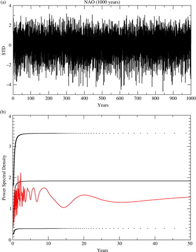
Further support for such an interpretation is obtained by examining a recent long-term integration by the MPI coupled climate model (Jungclaus et al., 2010). This model combines atmosphere, ocean and the carbon cycle. The actual model run included solar variability and aerosols from known volcanic eruptions. Fig. 2a shows NAO at monthly resolution for a 1000-yr long integration typical of pre-industrial conditions, and Fig. 2b shows the corresponding power spectrum. As can be seen, the random walk noise is well within the error bars (95% confidence interval) demonstrating a typical stochastic behaviour. As the European winter climate is strongly related to NAO both with respect to temperature and precipitation anomalies (Hurrell et al., 2003), we might, following Hunt and Elliott (2006) and Hunt (2007), conclude that climate variations on time scales shorter than say half a century is likely to be strongly affected by chance. It follows further that it is highly unlikely the variations in NAO have any useful predictive skill from year to year and even from month to month.

Fig. 2.  (a) NAO from a 1000-yr pre-industrial simulation calculated by the MPI coupled climate model (Jungclaus et al., 2010). NAO has been calculated as the average surface pressure at monthly mean values between the boxes (35°N, 45°N, 10°W, 70°W) and (45°N, 70°N, 10°W, 70°W). The model includes forcing from solar variability and volcanic aerosols from known eruptions. For information, see Jungclaus et al. (2010). The variation in greenhouse gas forcing is insignificant. (b) Power spectrum for the same function with the annual cycle removed, showing values from 1 month to 50 yr (red). The central solid line is the equivalent of a first-order auto-regressive process, AR(1). Upper and lower lines indicate 95% confidence interval. The result indicates that NAO is a red spectrum (random walk noise) and is fully dominated by internal processes. It should be noted that monthly extremes exist of more than 4.5 SD.

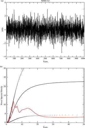
While NAO mainly influences the North Atlantic and Europe and primarily so during the winter, ENSO has a more far reaching influence as it affects the weather over a major part of the tropics as well as the Western Hemisphere (Allan et al., 1996). The major ENSO event 1997/98 warmed the global troposphere by almost 1°C making 1998 one of the warmest years in the observational records. A similar extreme event occurred in 1876/78. While ENSO has indication of a period of around 4 yr (Philander, 1990), it also incorporates considerable low-frequency variability, in particular, with respect to the amplitude of ENSO. Available observational records do not indicate any systematic variability or trends beyond the typical period of around 4 yr. Similar behaviour is indicated from longer integrations with coupled climate models as illustrated by results from a 1000-yr integration with the MPI coupled climate model. Figure 3a shows Nino 3.4 over 1000 yr, and Fig. 3b shows the corresponding power spectrum indicating a significant signal between 3 and 4.5 yr, while for shorter and longer periods the modelled ENSO shows up as a red spectrum. We consequently have indications that typical climate patterns in the atmosphere are stochastic except for a weak periodicity of around 4 yr for ENSO. There are indications in some observational records of longer periods of several decades, but the data records are to short or too inaccurate to indicate any significance (Cobb et al., 2003). We will therefore assume that the inter-annual variations of atmospheric circulation is inherently stochastic, and as a working hypothesis in this paper, it will assume that any longer-term trends and especially regional trends are likely to occur by chance or at least be strongly affected by chance. This is indeed the working principle for the fingerprint approach underlying the IPCC methodology of climate change attribution and where the approach has been trying to falsify stochastic long-term trends.

Fig. 3.  (a) ENSO determined from monthly mean surface temperature (5°N, 5°S, 90°W, 150°W), and Nino 3.4 determined from a 1000-yr simulation by the MPI coupled climate model (Jungclaus et al., 2010). The model includes forcing from solar variability and volcanic aerosols from known eruptions. For information, see Jungclaus et al. (2010). The variation in greenhouse gas forcing is insignificant. (b) Power spectrum for the same function showing values from 1 month to 50 yr (red). The central solid line is the equivalent of a first-order auto-regressive process, AR(1). Upper and lower lines indicate 95% confidence interval. There is a weak peak between 3 and 4.5 yr but for shorter and longer periods ENSO follows a random walk noise and is dominated by internal processes.

3. The European climate during the last 500 yr

Bengtsson et al. (2006) tested this stochastic hypothesis by examining near-surface temperature records for Europe covering the period 1500–2003 as had been compiled by Luterbacher et al. (2004) and Xoplaki et al. (2005). The temperature records by Luterbacher and Xoplaki are particularly useful, as temperature data has been compiled separately for each season. As can be seen in Bengtsson et al. (2006, Table 3), the coldest seasonal as well as the coldest decadal seasonal value occurs at very different times and indeed in different centuries. The coldest winter occurred in 1695/96, the coldest spring in 1785, the coldest summer in 1902 and the coldest autumn in 1912. A similar pattern is correspondingly found for the coldest seasonal decades. The extreme warm seasons on the other hand all occurred in the late 20th and early 21st century, with the exception of the autumn, but this occurred in fact in 2006 just after the end of the Luterbacher's and Xoplaki's data record. This is strongly suggestive of a dominant stochastic behaviour of the European near-surface temperature but with an indication of what can be interpreted as a superimposed warming trend showing up as an accumulation of the warmest seasons during the latest two decades of the more than 500-yr long temperature record. The accumulation of extreme warm events can thus be seen as a falsification of true stochastic climate and lend strong support to the forcing from the well-mixed greenhouse gases, lacking other credible alternatives.

Bengtsson et al. (2006) investigated a 500-yr coupled model integration (Roeckner et al., 2003, 2006) and used this to examine extreme or rare events. The 500-yr integration used pre-industrial radiative condition but was not exposed to any changes in the external forcing except the annual cycle for the whole period. The main focus was on the European area as the objective was to compare the statistics from observations from Luterbacher et al. (2004) and Xoplaki et al. (2005) with the statistics of the model. Table 2 reproduced from Bengtsson et al. (2006) depicts mean values, standard deviations and extremes.

Table 2. Observed land surface temperature 1500–1900 for the area 35N–70N and for 25W–40E from Luterbacher et al. (2004). The standard deviation, SD, for the last 100 yr is 0.53, suggesting that the variance is underestimated in the earlier record. The same for the model results, ECHAM5/ MPI-OM. Results have been calculated from a 500-year climate simulation without any changes in external forcing. Values from Bengtsson et al. (2006). Values are, in both cases, average values for the whole year and winter (DJF) and summer (JJA), respectively. The actual years of the extreme temperatures are indicated (units in °C). The coldest winter in the model run corresponds to 4.2 SD and the warmest summer to 3.8 SD. The corresponding values from the observational data set are 3.3 SD and 2.9 SD, respectively

		Luterbacher et al. (2004)			Bengtsson et al. (2006)
	Observations Annual	DJF	JJA	Model Annual	DJF	JJA
Mean	8.1	−2.3	16.8	7.4	−2.3	17.0
SD	0.41	1.15	0.47	0.55	1.23	0.55
Min (year)	6.6 (1695)	−5.7 (1695/96)	15.6 (1821)	5.4 (16)	−7.5 (17/18)	15.6 (170)
Max (year)	9.4 (1822)	−0.1 (1842/43)	18.2 (1757)	9.4 (78)	1.5 (51/52)	19.1 (459)
Max–min	2.8	5.6	2.6	4.0	8.9	3.5

Generally, there is a considerable degree of similarity between model and observations although the standard deviation of the model run is somewhat larger. It is judged that the variance of the earlier observed data is under-estimated as the last 100 yr are closer to the model simulation. In Figs. 4 and 5, partly from Bengtsson et al. (2006, Figs. 8 and 9), we note that there are typical similarities between extreme cold winters as well as extreme warm summers in observations and in model simulation, in Fig. 4 we also compare the model result with a recent cold winter, 2009/2010, and in Fig. 5 with the very warm European summer of 2003. A very cold European winter is also colder than normal over northern Russia but warmer than normal in the Arctic and in the tropical Pacific. The reason to the warmer than normal conditions in the Arctic is related to the large deviation in the position of the Atlantic storm track. In the typical circulation pattern that leads to cold weather in Europe during winter, the storm tracks are often split in a northerly and a southerly branch transporting warm air into the Arctic and blocking the warmer air to reach northern and central Europe.

Fig. 4.  (a) The temperature anomaly of the 10 coldest winters (DJF) for a model integration over 500 yr using pre-industrial forcing conditions. (b) The observed temperature anomaly for the winter 2009/2010 relative to the mean temperature 1990–2010. The cold anomaly covers the major part of the northern Eurasia as well as the major part of US and southern and western Canada. The Arctic is warmer than normal. There are considerable similarities between the observed and model simulated pattern, suggesting similar anomaly circulation pattern. [(b) Retrieved from http://data.giss.nasa.gov/gistemp/maps/]

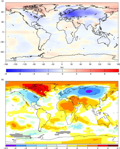
Fig. 5.  (a) The temperature anomaly for the 10 warmest summers (JJA) for the same 500-yr model integration. (b) The temperature anomaly for the summer of 2003 relative to the mean temperature 1990–2010. The extreme warm anomaly over Europe is connected to a band of warmer than normal sea surface temperatures over the central Atlantic. There is a region with colder than normal conditions over the central part of the Asian mainland. There are several similarities between the model anomalies but not as pronounced as for the winter case. [(b) Retrieved from http://data.giss.nasa.gov/gistemp/maps/]

4. Summary and concluding remarks

While many generally have a sceptical attitude to climate model simulations, we probably tend to be less sceptical to observational data. In fact, observational data, in particular older data sets or so-called observational reconstructions, are often considered to be a sort of replacement for true observations. There are indications that reconstructed data sets because of insufficient resolution in time and space, often underestimate climate variability. Another problem is a tendency by researchers to have conceptual ideas about the causes of climate variations that inadvertently influences the interpretation of climate events in terms of anticipated external causes.

An example here is the reconstruction of the solar irradiation records that was based on a relation between solar irradiation and sunspots, normalised by a prolonged sunspot minimum between 1645 and 1715, the so-called Maunder minimum. This partly coincided with periods of low winter temperatures in Europe (Eady, 1976) that strongly underpinned the notion of marked variations in total solar irradiation related to sunspots. With the support of available temperature records, seen as an indication of the solar influence, long-term records of total solar irradiation were compiled. These reconstructed solar irradiation data (e.g. Lean et al., 1995) covering several centuries were then used by climate modellers that, unaware how the irradiation data set had been compiled, not surprisingly were able to broadly reproduce some of the extreme periods including the colder ones during the Maunder minimum (e.g. Cubasch et al., 1997) and was considered as a clear indication of a cause–effect relation. This example of circular reasoning bewildered climate scientists for a considerable time and is still being used as an example that variations in solar irradiation have controlled the climate of the past millennia. Furthermore, it is seen as a main driver for present climate warming. However, as has been shown based on satellite based observations since 1978 (e.g. Fröhlich, 2012), there is no well-established relationship between solar irradiation and sunspot numbers, and solar variations are generally an order of magnitude smaller than the increase is the forcing from the well-mixed greenhouse gases over the last three solar cycles (Lockwood, 2012).

Similar tendency of circular reasoning can also be noticed in the way the effect on radiation by tropospheric aerosols are used in modelling and in that connection as a tool to adjust external forcing to obtain a better agreement with the observed temperature evolution during the last century or so (Kiehl, 2007). There is a temptation by many scientists and laymen alike to look for simple and linear relations between cause and effect in climate. Unfortunately, because of the strong chaotic component as identified in model experiments and almost daily in weather prediction, not the least by operational ensemble predictions, considerable periods of time are needed to generate a sufficient amount of data to determine a sufficient volume of information to comprehensively determine and sample climate in a statistical sense.

Several arguments have been put forward to question this critique suggesting that models are likely to overestimate internal variability. I do not consider this to be a valid argument as similar phenomena also occur in experimental studies; Edward Lorenz study of the predictability of simple systems (Lorenz, 1963a, 1963b) was encouraged by the physicist Raymond Hide's work on a rotating annulus and the identification of a marked hysteresis effects (Hide, 1953) and similar studies by Fultz et al. (1959).

I would rather argue that models rather are likely to underestimate the magnitude of internal variations and in particular longer cycles that include the deep ocean circulation and energy exchange with upper layers of the ocean.

Internal climate variability and limited climate predictability are closely related to the issue of the uniqueness of climate. Claussen (1998) has undertaken a study to explore the uniqueness of the Earth's climate zones assuming that the annual cycle of the ocean surface temperature is given. In an experimental demonstration the initial vegetation patterns affecting land albedo and evapotranspiration were fully distorted from the present by, for example, making Sahara into a tropical forest and Amazonas into a desert region. After a number of successive integrations after which the vegetation zones were re-determined based on changes in the local monthly temperature and precipitation, it was finally found that the climate zones gradually converged to essentially the present climate and the selected extreme initial conditions were completely changed to the presently observed. From this, we might conclude that the basic atmospheric dynamical conditions under the present radiation forcing did essentially determine the present typical global climate zones. Let us now assume that we also had decided to let the oceans be put at rest and with the same temperature everywhere. Because of the thermal and dynamical inertia of the oceans, such an experiment is extremely demanding computationally and has not yet been undertaken. However, I am not convinced that after some several thousand years of integration that we would arrive at the present climate. If we would start with, for instance, the mean temperature of the ocean (ca. +4°C) it could well happen that we have to go through a very different climate for several thousand years before we might reach something that might bear some similarity to our present climate. In my opinion, it is a great pity that not more of such fundamental studies of climate are undertaken and perhaps some of the huge computational resources now devoted to IPCC simulations could be used for a more general class of climate investigations like the many fundamental studies that are so common in astronomy today, such as the evolution of the universe and simulation studies of the dynamics of black holes.

5. Acknowledgements

I am very grateful for the opportunity to have known Bert Bolin. I met him frequently over a considerable period of time, first as a student of meteorology, then over many years at different places and in different capacities until the very last year of his life. He was always available for advice and encouragement, and I very much miss his sound judgement in key science matters. Bert Bolin had the unusual ability to combine a genuine understanding and deep knowledge of weather and climate, in details as well as in a broad sense, combined with a strong conviction to bring this knowledge to the benefit of mankind. Few individuals have been as successful in this respect as Bolin, and there is huge gratitude for his outstanding contributions to science, international cooperation and society. He set an example for us all to follow. I am most grateful to my colleague Dr. K. I. Hodges for undertaking the statistical calculations used in this paper and to Dr. J. H. Jungclaus at the Max Planck Institute for Meteorology in making the MPI climate simulation available.

References

- Allan, R, Lindesay, J and Parker, D. 1996. El Niño: Southern Oscillation and Climate Variability. CSIRO Publishing, Collingwood, Vic., Australia, 416. pp.
- Baldwin, M. P, Gray, L. G, Dunkerton, T. J, Hamilton, K, Hayes, P. H. and co-authors. 2001, The quasi-biennial oscillation. Rev. Geophys. 39: 179–229. 10.3402/tellusb.v65i0.20189.
- Bengtsson, L. 2001. Uncertainties of global climate prediction. In: Global Biogeochemical Cycles in the Climate System. Schulze, E-D., Heimann, M., Harrison, S., Holland, E., Lloyd, J. and co-editors). Academic Press San Diego, 350 pp..
- Bengtsson L, Hodges K. I, Roeckner E, Brokopf R. On the natural variability of the pre-industrial European climate. Clim. Dyn. 2006; 26: 743–760. 10.3402/tellusb.v65i0.20189.
- Boer, G. J and Yu, B. 2003. Climate sensitivity and climate state. Clim. Dyn. 21: 167–176. 10.3402/tellusb.v65i0.20189.
- Charney J, Fjörtoft R, Von Neumann J. Numerical integration of the barotropic vorticity equation. Tellus. 1950; 2: 237–254. 10.3402/tellusb.v65i0.20189.
- Claussen M. On multiple solutions of the atmospheric-vegetation system in present-day climate. Glob. Change Biol. 1998; 4: 549–559. 10.3402/tellusb.v65i0.20189.
- Cobb, K. M., Charles, C. D, Cheng, H and Edwards, R. L. 2003. El Niño/Southern oscillation and tropical Pacific climate during the last millennium. Nature. 424: 271–276. 10.3402/tellusb.v65i0.20189.
- Compo, G. P, Whitaker, J. S, Sardeshmukh, P. D, Matsui, N, Allan, R. J. and co-authors. 2011. Review article the twentieth century reanalysis project. Q. J. R. Meteorol. Soc. 137: 1–28. 10.3402/tellusb.v65i0.20189.
- Cubasch U, Voss R, Hegerl G. C, Waszkewitz J, Crowley T. J. Simulation of the influence of solar radiation variations on the global climate with an ocean-atmosphere general circulation model. Clim. Dyn. 1997; 13: 757–767. 10.3402/tellusb.v65i0.20189.
- Dee, D. P, Uppala, S. M, Simmons, A. J, Berrisfoord, P, Poli, P. and co-authors. 2011. The ERA-Interim reanalysis: configuration and performance of the data-assimilation system. 137: 553–597. 10.3402/tellusb.v65i0.20189.
- Eady J. A. The Maunder minimum. Q. J. R. Meteorol. Soc. 1976; 192: 1189–1202. 10.3402/tellusb.v65i0.20189.
- Fröhlich, C. 2012. Total solar irradiance observations. Science. 33: 453–473. 10.3402/tellusb.v65i0.20189.
- Fultz, D, Long, R. R, Owens, G. V, Bohan, W, Kaylor, R. and co-authors. 1959. Studies of thermal convection in a rotating cylinder with some implications for large-scale atmospheric motions. Surv. Geophys. 4: 104.
- Hide R. Some experiments on thermal convection in a rotating liquid. Meteorol. Monogr. 1953; 79: 161.10.3402/tellusb.v65i0.20189.
- Hunt B. G. Climate outliers. Q. J. R. Meteorol. Soc. 2007; 27: 139–156. 10.3402/tellusb.v65i0.20189.
- Hunt B. G, Elliott T. J. Climate trends. Int. J. Clim. 2006; 26: 567–585. 10.3402/tellusb.v65i0.20189.
- Hurrell, J. W., Kushnir, Y., Ottersen, G. and Visbeck, M. 2003. The north Atlantic oscillation: climatic significance and environmental impact. Geophys. Monogr. Ser. 134: 279. 10.3402/tellusb.v65i0.20189.
- Jungclaus, J. H, Lorenz, S. J, Timmreck, C, Reick, C. H, Brovkin, V. and co-authors. 2010. Climate and carbon-cycle variability over the last millennium. 6: 723–737. 10.3402/tellusb.v65i0.20189.
- Kiehl J. Twentieth century climate model response and climate sensitivity. Clim. Past. 2007; 34: L22710.10.3402/tellusb.v65i0.20189.
- Kloster, S, Dentener, F, Feichter, J, Raes, F, Lohmann, U. and co-authors. 2010. A GCM study of future climate response to aerosol pollution reductions. Geophys. Res. Lett. 34: 1177–1194. 10.3402/tellusb.v65i0.20189.
- Kollek M, Grieser J, Beck C, Rudolf B, Rubel F. World Map of the Köppen-Geiger climate classification updated. Clim. Dyn. 2006; 15: 259–263.
- Köppen, W. 1884. Die Wärmezonen der Erde, nach der Dauer der heissen, gemässigten und kalten Zeit und nach der Wirkung der Wärme auf die organische Welt betrachtet. Meteorol. Zeitschr. 1: 215–226. (in German).
- Köppen, W. 1900. Versuch einer Klassifikation der Klimate, vorzugweise nach ihren Beziehungen zur Pflantzenwelt. Meteor. Zeitschr. 6: 593–611., 657–679 (in German).
- Köppen, W. 1936. Das geographische System der Klimate. In: Handbuch der Klimatologie. Köppen, W. and Geiger, R. Band 5, Teil C. Gebrüder Bornträger, Berlin (in German).
- Lean J, Beer J, Bradley R. Reconstruction of solar irradiance since 1610: implications for climate change. 1995; 22: 3195–3198. 10.3402/tellusb.v65i0.20189.
- Lenton, T. L, Held, H, Kriegler, E, Hall, J. W, Lucht, W. and co-authors. 2008. Tipping elements in the earth's climate system. Geophys. Res. Lett. 105: 1786–1793. 10.3402/tellusb.v65i0.20189.
- Lindzen R. S, Holton J. R. A theory of the quasibiennial oscillation. PNAS. 1968; 25: 1095–1107.
- Lockwood, M. 2012. Solar influence on global and regional climates. J. Atmos. Sci. 33: 503–534. 10.3402/tellusb.v65i0.20189.
- Lorenz E. N. Deterministic non-periodic flow. Surv. Geophys. 1963a; 20: 130–141.
- Lorenz E. N. The mechanisms of vacillation. J. Atmos. Sci. 1963b; 20: 448–464.
- Lorenz E. N. Atmospheric predictability experiments with a large numerical 22 model. J. Atmos. Sci. 1982; 34: 505–513. 10.3402/tellusb.v65i0.20189.
- Luterbacher J, Dietrich D, Xoplaki E, Grosjean M, Wanner H. European seasonal and annual temperature variability, trends and extremes since 1500. Tellus. 2004; 303: 1499–1503. 10.3402/tellusb.v65i0.20189.
- Pfeffer, R. L. 1960. Dynamics of Climate: Proceedings. Symposium Publications Division, Pergamon Press: Oxford, New York.
- Philander, S. G. H., 1990. El Niño, La Niña and the Southern Oscillation. Academic Press: San Diego CA.
- Roeckner, E, Bäuml, G, Bonaventura, L, Brokopf, R, Esch, M. and co-authors. 2003. The atmospheric general circulation model ECHAM 5. Part I: model description. 127.
- Roeckner, E, Brokopf, R, Esch, M, Giorgetta, M, Hagemann, S. and co-authors. 2006, Sensitivity of simulated climate to horizontal and vertical resolution in the ECHAM5 atmosphere model. MPI-Report 349. 19: 3771–3791. 10.3402/tellusb.v65i0.20189.
- Sanderson M. The classification of climates from Pythagoras to Koeppen. J. Clim. 1999; 80: 669–673.
- Xoplaki, E, Luterbacher, J, Paeth, H, Dietrich, D, Steiner, N. and co-authors. 2005. European spring and autumn temperature variability and change of extremes over the last half millennium. Bull. Am. Met. Soc. 32: L15713. DOI: 10.3402/tellusb.v65i0.20189.