On the use of MOZAIC-IAGOS data to assess the ability of the MACC reanalysis to reproduce the distribution of ozone and CO in the UTLS over Europe

Abstract

MOZAIC-IAGOS data are used to assess the ability of the MACC reanalysis (REAN) to reproduce distributions of ozone (O₃) and carbon monoxide (CO), along with vertical and inter-annual variability in the upper troposphere/lower stratosphere region (UTLS) over Europe for the period 2003–2010. A control run (CNTRL, without assimilation) is compared with the MACC reanalysis (REAN, with assimilation) to assess the impact of assimilation. On average over the period, REAN underestimates ozone by 60 ppbv in the lower stratosphere (LS), whilst CO is overestimated by 20 ppbv. In the upper troposphere (UT), ozone is overestimated by 50 ppbv, while CO is partly over or underestimated by up to 20 ppbv. As expected, assimilation generally improves model results but there are some exceptions. Assimilation leads to increased CO mixing ratios in the UT which reduce the biases of the model in this region but the difference in CO mixing ratios between LS and UT has not changed and remains underestimated after assimilation. Therefore, this leads to a significant positive bias of CO in the LS after assimilation. Assimilation improves estimates of the amplitude of the seasonal cycle for both species. Additionally, the observations clearly show a general negative trend of CO in the UT which is rather well reproduced by REAN. However, REAN misses the observed inter-annual variability in summer. The O₃–CO correlation in the Ex-UTLS is rather well reproduced by the CNTRL and REAN, although REAN tends to miss the lowest CO mixing ratios for the four seasons and tends to oversample the extra-tropical transition layer (ExTL region) in spring. This evaluation stresses the importance of the model gradients for a good description of the mixing in the Ex-UTLS region, which is inherently difficult to observe from satellite instruments.

• ozone
• carbon monoxide
• UTLS
• mixing processes
• MOZAIC
• MACC reanalysis

This paper is part of a Special Issue on MOZAIC-IAGOS in Tellus B celebrating 20 years of an ongoing air chemistry climate research measurement from airbus commercial aircraft operated by an international consortium of countries. More papers from this issue can be found at http://www.tellusb.net

1. Introduction

Ozone (O₃) and carbon monoxide (CO) are two important trace gases in the atmosphere and key species for both air quality and climate issues. Tropospheric ozone is a key trace gas in the atmosphere with a central role in the tropospheric oxidation of methane (CH₄), CO and non-methane volatile organic compounds (NMVOC) in the presence of nitrogen oxides (NOx) (Crutzen, 1974; Derwent et al., 1996). Tropospheric ozone is the third most important greenhouse gas (IPCC, 2013) after carbon dioxide (CO₂) and methane (CH₄). CO also plays a major role in the chemistry of the troposphere, affecting the concentrations of oxidants such as the hydroxyl radical (OH) and ozone (Wotawa et al., 2001). It is classified as an indirect greenhouse gas (IPCC, 2013) since it is a chemical precursor of CO₂ and ozone. It is estimated that about two-thirds of CO originates from anthropogenic activities (Van der Werf et al., 2010), principally biomass burning. Emissions of biogenic and anthropogenic volatile organic compounds (VOC) also contribute significantly to CO (Stein et al., 2014).

The distribution of ozone and CO in the extra tropical upper troposphere–lower stratosphere (Ex-UTLS, Gettelman et al., 2011) is of particular interest for global budget analyses and also for climate impact issues as small changes in the abundances of gases in the upper troposphere (UT) have relatively large radiative effects (Forster et al., 1997; Aghedo et al., 2011; Riese et al., 2012). The distribution of ozone and CO in the Ex-UTLS is controlled by the proximity of the tropospheric and stratospheric reservoirs with the LS being an important source of ozone for the UT via dynamical processes such as stratospheric intrusions (Gettelman et al., 2011). With strong vertical gradients, ozone and CO change sharply across the tropopause (Schmidt et al., 2010). Given the complex but important role of the UTLS, it is essential for global models to reproduce the observed distribution of ozone and CO in this region and to be able to attribute its origin and cause of variability.

A few observing programmes are designed to assess the global distribution of ozone and CO in the UTLS. Monitoring tropospheric ozone started in the 1960s with ozone sondes which were relatively sparse in space and time (3–12 per month) over about 40 northern hemispheric sites (e.g. Logan, 1985). Later, remote sensing satellites allowed the retrieval of tropospheric ozone on the global scale, but with considerable uncertainties (e.g. Fishman et al., 1990). CO has also been measured by different space-borne instruments since the end of the 1990s, beginning with the MOPITT instrument (Measurements Of Pollution In The Troposphere) (Edwards et al., 1999). In-situ observations of CO are available from surface network (e.g. GAW network) and regular aircraft campaigns (Novelli et al., 2003). In situ measurements can achieve the high spatial and temporal resolution needed for assessing the distributions of ozone and CO, their interrelationships in the Ex-UTLS and the thickness of the tropopause transition layer (Pan et al., 2007a, 2007b; Brioude et al., 2008; Tilmes et al., 2010). The use of CO–O₃ correlations was first applied to research aircraft data (Fischer et al., 2000; Hoor et al., 2002; Pan et al., 2004) as well as on regular in-situ observations with CARIBIC (Zahn et al., 2000, 2002). The vertical extent of the ExTL from CO–O₃ correlations and tropopause coordinates was first deduced based on STREAM data and SPURT data (Hoor et al., 2002, 2004; Zahn et al., 2002). Since December 2001, the MOZAIC programme (Measurement of OZone and water vapour by in-service AIrbus airCraft; Marenco et al., 1998) and its successor IAGOS (In-Service Aircraft for a Global Observing System; Petzold et al., 2015, www.iagos.fr for data access) have measured ozone and CO (and other compounds) simultaneously on board a fleet of commercial aircraft (5–20 aircraft), sampling the Ex-UTLS region between 9 and 12 km altitude with high vertical (28 m) and horizontal (1 km) resolution.

Global chemistry transport models (CTMs) enhance our understanding of the processes controlling the distributions and variability of chemical species such as ozone and CO (e.g. Kanakidou et al., 1999; Shindell et al., 2006a; Naik et al., 2013; Stevenson et al., 2013). For CO in particular, Shindell et al. (2006a) have shown that the variability among models is large and that significant underestimations are found notably in the extra-tropical Northern Hemisphere. Sources of uncertainties are diverse and include emissions inventories and emissions injection height estimates which affect long-range transport and chemistry (Stein et al., 2014). The magnitude of photochemical production and destruction within the troposphere along with import from stratosphere are major sources of biases to observations. Data assimilation can improve model descriptions of atmospheric composition. Reducing these uncertainties and providing high quality ozone and CO distributions with a specific focus on the ability to describe long-range transport of pollution was one of the main objectives of the successive GEMS (Global Earth-system Modelling using Space and in-situ data; 2005–2009; Hollingsworth et al., 2008) and MACC (Monitoring Atmospheric Composition and Climate; 2009–2015: www.copernicus-atmosphere.eu) projects in preparation for the Copernicus Atmospheric Monitoring Service (CAMS) (Flemming et al., 2009). Within this framework, the ECMWF's (European Centre for Medium-range Weather Forecast) Integrated Forecast System (IFS) model has been coupled with MOZART-3 (Kinnison et al., 2007; Stein et al., 2012, 2014) to form a reanalysis of global atmospheric composition for the years 2003–2012, making use of the assimilation of satellite data from different instruments. Details are given by Inness et al. (2013) and evaluation of the data set for reactive gases is performed also by Eskes et al. (2015) and Katragkou et al. (2015). Further validation reports can be found on www.copernicus-atmosphere.eu/quarterly_validation_reports.

The MACC reanalysis provides the first global data set combining observational information on several reactive gas species as well as aerosols and has lower biases than the ERA-Interim reanalysis (Dee et al., 2011) for ozone.

The objective of this study is to present an evaluation of the MACC reanalysis with simultaneously measured ozone and CO mixing ratios from the MOZAIC-IAGOS programme. The evaluation is focused on the Ex-UTLS region over Europe, since this is the best-sampled region in the data base. Specifically, we will evaluate the added value of the assimilated satellite data in the reanalysis, by comparing the evaluation results against a control version of the model which does not apply data assimilation. This article complements previous studies which used MOZAIC data to evaluate the different versions of the GEMS and MACC models. Elguindi et al. (2010) used MOZAIC profiles to investigate the transport of biomass burning products between North America and Europe during summer 2004. Ordoñez et al. (2010), focused on tropospheric ozone and CO profiles during the heat wave event in summer 2003 in Europe. Stein et al. (2014) analysed the wintertime low bias of Northern Hemisphere CO found in global simulations from Model for Ozone and Related chemical Tracers (MOZART), while Inness et al. (2013) presented an evaluation of the MACC reanalysis mainly for the free troposphere and stratosphere. In this article, we use the high density and frequency of MOZAIC-IAGOS high resolution to explore the ability of the model (1) to reproduce the observed variability and (2) to reproduce the mixing processes within the Ex-UTLS using O₃/CO scatter plots (as done by Hoor et al., 2002; Pan et al., 2007a, 2007b; Brioude et al., 2008; Barré et al., 2013).

This paper contributes to the set of various evaluation procedures of the MACC system with other independent networks of in-situ data (NDACC, GAW) as it presents evaluation with simultaneous ozone and CO data in the critical Ex-UTLS region. Our objective is also to ‘pave the road’ for further developments on a long-term survey for quantifying model improvements in the frame of the CAMS and the expansion of the IAGOS programme including additional sampled regions and additional measured compounds. Sections 2 and 3 introduce the model and observational data as well as the methodology applied to perform a quantitative assessment of the differences between observations and model outputs. Then, Section 4 presents the evaluation of seasonal and annual distributions, and mixing processes in the Ex-UTLS of the MACC reanalysis and its control run. Section 5 presents the conclusions.

2. Data

2.1. MOZAIC-IAGOS data

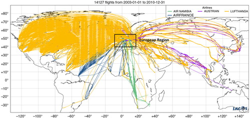
The MOZAIC programme started in 1994 with five aircraft from European airlines (Marenco et al., 1998 and www.iagos.fr/mozaic) and was designed to measure ozone and water vapour from the beginning, and additionally CO (since 2001) and NOy (2001–2005). Figure 1 shows the map of the flights between 2003 and 2010. IAGOS as successor programme started in July 2011 (www.iagos.org; WMO Bulletin, 2014; Petzold et al., 2015) and six aircraft have been flying so far. The data base is now called the IAGOS data base and includes former MOZAIC data.

Fig. 1 Map of MOZAIC flights for the studied period (2003–2010). The black square corresponds to the European region (40°N–55°N, 10°W–15°E) used in our study.

Ozone and CO have been measured simultaneously since December 2001 on board five aircraft. The measurements of ozone and CO use improved commercial analysers with UV photometer and IR absorption technique, respectively. Measurements of ozone are taken every 4 seconds from take-off to landing and the measurement's total uncertainty is estimated at±2 ppbv±2%. Measurements of CO are taken every 30 seconds and the measurement's total uncertainty is±5 ppbv±5%. Details on the measurement technique and uncertainties can be found in Marenco et al. (1998) and Thouret et al. (1998) for ozone, and Nédélec et al. (2003) for CO, and more recently in Nédélec et al. (2015). For all the flights, the same instruments and the same calibration procedures (following the WMO-GAW recommendations, www.wmo.int/pages/prog/arep/gaw/gaw-reports.html) are used.

To ensure the statistical significance of the study, we focus on the region of Europe (40°N–55°N, 10°W–15°E) where the frequency of the measurements is the most intensive thanks to the European airlines involved in the programme (departing/landing from Paris, London, Frankfurt, Munich, Düsseldorf and Vienna). In total, 14 127 flights took place over Europe in the UTLS for the period 2003–2010, which means 1766 per year, 147 per month and 4 per day on average (Fig. 2).

Fig. 2 Number of flights per month over the European region (Paris, London, Frankfurt, Munich, Düsseldorf and Vienna) from Jan 2003 to Dec 2010.

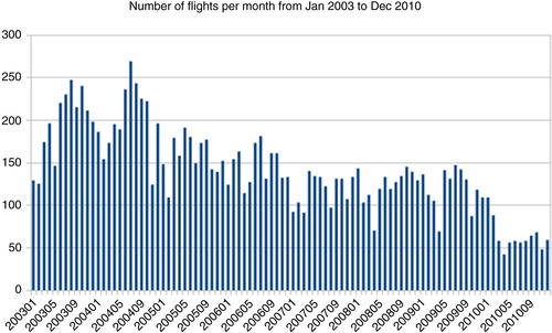
Although the number of flights per month decreased with time because of the decrease of the number of aircraft (from 5 in 2003 to 2 in 2010), there is still at least one flight per day as the number of flights per month is never less than 30. However, between April and August 2010, there were no ozone and CO data because of technical problems in the transition phase between MOZAIC and IAGOS programmes. Therefore, 2010 will be excluded from our statistical evaluation.

2.2. MACC reanalysis

The MACC Reanalysis (REAN) of atmospheric composition covers the years 2003–2012 and was produced with ECMWF's Global IFS model and data assimilation system coupled to the CTM MOZART (Stein et al., 2012), using the coupling software OASIS4 (Ocean Atmosphere Sea Ice Soil version 4). The resolution of IFS is T255 corresponding to 80 km horizontal resolution. The vertical resolution is 60 vertical levels. The resolution of MOZART is 1.125°×1.125°. Further details about the model configuration are given in Flemming et al. (2009) and Inness et al. (2013).

Satellite data from GOME (Global Ozone Monitoring Experiment), MIPAS (Michaelson Interferometer for Passive Atmospheric Sounding), MLS (Microwave Limb Sounder), OMI (Ozone Monitoring Instrument), SBUV/2 (Solar Backscatter UltraViolet), SCIAMACHY (SCanning Imaging Absorption SpectroMeter for Atmospheric CHartographY) were used in the assimilation for ozone_. Total columns of ozone and stratospheric profile data are assimilated and the impact on tropospheric ozone comes from the residual of the two. IASI (Interféromètre Atmosphérique de Sondage Infrarouge) and MOPITT were used in the assimilation for CO. In the MACC system total column and profile data are assimilated. The profile data are presented to the data assimilation system as a stack of partial columns (each bounded by a top and bottom pressure value, unit kg/m²) and can hence be treated in the same way as total column data by the observation operator. The model's background column value at the time and location of the observations is either calculated as a simple vertical integral between the top and the bottom pressure given by the partial or total column or by using averaging kernels if available for the data (see Inness et al., 2013 for more details).

Emission inventories include MACCity (MACC/CityZEN EU projects) for anthropogenic emissions (Granier et al., 2011), GFAS (Global Fire Assimilation System, Kaiser et al., 2012) and GFED (Global Fire Emission Database, Van der Werf et al., 2010) for the biomass burning, MEGAN (Model of Emissions of Gases and Aerosols from Nature, Guenther et al., 2006) for the biogenic emissions and POET (Precursors of Ozone and their Effects in the Troposphere) for other natural emissions (Inness et al., 2013).

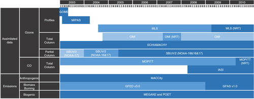
Figure 3 shows the time evolution of the assimilated ozone and CO data and the emissions inventories from 2003 to 2010. It shows, for example, that no ozone profile data were available in April, May and June 2004, and that the assimilation of IASI CO retrievals started in April 2008. When multiple satellites observing the same component were assimilated in REAN a variation bias correction scheme was applied to some of the datasets while data from one instrument were used uncorrected per species, to act as an anchor for the bias correction (Inness et al., 2013). MOPITT was used as anchor for CO and SBUV/2 data were used as anchor for ozone. Unfortunately, using SBUV/2 as anchor could not stop the bias correction drifting for individual MLS layers which had a higher vertical resolution, and this led to a drift in the REAN ozone field. When this was discovered during the reanalysis production, the bias correction was turned off for MLS and MLS was used uncorrected in REAN from 1 January 2008 onwards.

Fig. 3 Evolution of assimilated data and emissions sources (in blue cells) used in REAN from 2003 to 2010. MOPITT was used as anchor for CO and SBUV/2 data were used as anchor for ozone. Using SBUV/2 as anchor could not stop the bias correction drifting for individual MLS layers. When this was discovered during the reanalysis production, the bias correction was turned off for MLS and MLS was used uncorrected in REAN from 1 January 2008 onwards.

2.3. MACC control run

The MACC control run (CNTRL) is a MOZART-3 stand-alone simulation driven by IFS meteorology and applying the same settings as MOZART in REAN in terms of model code, resolution, and emissions, but without constraints on chemical composition from observations. It is suitable for assessing the impact of the data assimilation on the modelled distribution of ozone and CO from 2003 to 2010. More information about CNTRL can be found in Inness et al. (2013). Because the control run only covered the years 2003–2010, the comparisons in this paper are limited to this period.

3. Methodology

3.1. Observed and modelled data in the Ex-UTLS

To make observational data and the model directly comparable, the model fields were first linearly interpolated to the locations of the observations in space (latitude, longitude and pressure) and time. Potential vorticity is calculated systematically for each measurement in the MOZAIC database using the Lagrangian particle dispersion model FLEXPART (Stohl et al., 2005) to associate each measurement with PV from the ECMWF's operational analysis.

We defined the Ex-UTLS relative to the dynamical tropopause as the pressure level of the potential vorticity equal to 2PVU in the mid-latitudes (Potential Vorticity Units: 1 PVU = 10⁻⁶ m²s⁻¹Kkg⁻¹) (Holton et al., 1995; Bethan et al., 1996). The measurements and model data were then assigned to two bins as detailed in Thouret et al. (2006). The UT gathers measurements with a pressure (p_UT) satisfying the criteria p_2pvu+75 hPa > p_UT>p_2pvu+15 hPa, where p_2pvu is the pressure of the 2 PVU tropopause. The LS gathers measurements with a pressure (p_LS) satisfying p_LS<p_2pvu–45 hPa. The upper bound of p_LS is the cruise altitude of the aircraft which is always at around 12 km or 196 hPa.

The criteria used to attribute measurements to UT or LS was applied to both the observations and the modelled fields after their spatial and temporal interpolation to the flight-track.

There should not be a difference in the dynamical tropopause in the MOZAIC analysis and the tropopause from the model as both are based on the ECMWF operational model. The underlying physics and dynamics should be the same in both the operational analysis used to calculate PV and the physics and dynamics in the MACC reanalysis. Differences concern the resolution. In 2003, the ECMWF operational analysis had a resolution of T511 (0.3°) with 60 levels in the vertical. In 2006, the horizontal and the vertical resolutions were increased to T799 (0.2°) and 91 levels, respectively. Small differences in tropopause height between the MACC reanalysis and the ECMWF operational analysis may result from different radiative heating, due to the differences in the chemistry around the tropopause.

To assess the ability of REAN to reproduce the distributions of ozone and CO in the UTLS region over Europe, we used several well-known statistical parameters which are complementary. These are (1) the mean bias (MB), (2) the standard deviation (σ), the correlation coefficient (R) and the unbiased root mean square error (RMSD′), as summarised in Taylor diagrams, and (3) the probability density function (PDF). The next section gives further details on these tools.

3.1.1. Mean bias. The MB is used to quantify directly the differences in ozone and CO mixing ratios in ppbv between REAN or CNTRL and MOZAIC-IAGOS. Here, we use the monthly mean.1

where M corresponds to ozone or CO mixing ratios from models (i.e. REAN or CNTRL) and O corresponds to ozone or CO mixing ratios from observations (i.e. MOZAIC-IAGOS). The overbar refers to the monthly mean. MB is also calculated with yearly means of M and O, and is called MB_yr.

3.1.2. Taylor diagram

The standard deviation (σ), the correlation coefficient (R) and the unbiased root mean square (RMSD′) are very useful tools for a further quantitative evaluation of REAN and CNTRL with respect to MOZAIC-IAGOS. They are used here to assess the ability of the models to reproduce the seasonal cycle of each year of the time period (2003–2009). Discussion on the inter-annual variability of the seasonal cycle is also based on such diagrams.

The three statistics parameters are given for each year and have been calculated from monthly averages of observations and of model data matched to flight tracks.

R is a score used here to test the agreement in phase of the seasonal cycle [eq. (2)] between the models and the observations, while σ is used to quantify the amplitude of the seasonal cycle as it is explained in Taylor (2001). If , REAN or CNTRL overestimates (underestimates) the observed amplitude of the seasonal cycle. Here, the phase is defined as the month for which the mixing ratio of gas maximises and the amplitude is defined as the difference between the maximum and the minimum of the mixing ratio of gas (Taylor, 2001).2

where and are the annual mean values and and are the standard deviations of M and O from the monthly mean values. Here N equal to 12 as it is the number of monthly values in each year.

RMSD′ is a measure used to give global errors of REAN or CNTRL in reproducing the seasonal cycle compared to MOZAIC-IAGOS removing any information about the possible MB_yr of REAN or CNTRL with respect to MOZAIC-IAGOS [eq. (3)].3

The unbiased RMSD (RMSD') is equal to the total RMSD if there is no MB_yr between models and observations [eq. (4)]4

where the total RMSD is a measure of the average magnitude of the difference between models and observations [eq. (5)]5

Taylor (2001) have proposed to summarise the σ, R and RMSD′ on one polar coordinate diagram, called a Taylor diagram (for example Fig. 7). The angle corresponds to the inverse of the cosine of R (i.e. 0° corresponds to R=1). The radial axis corresponds to σ. The distance between points of models (i.e. R and σ of REAN or CNTRL) and points of observations taken as references (i.e. R and σ of MOZAIC-IAGOS) corresponds to RMSD′. In particular, we have used the normalised Taylor diagram for which the points of MOZAIC-IAGOS (the reference) have polar coordinates R=1 and σ=1. The smaller the distance to this point, the better is the model. However, we must be careful because, as mentioned above, no information on MB_yr can be read on this diagram (Jolliff et al., 2009). Indeed, Taylor diagram and MB_yr are complementary information to summarise the performance of the model (Taylor, 2001).

3.1.3. O₃–CO PDF

As ozone and CO are measured simultaneously by MOZAIC-IAGOS, we can compare the relationships between both species simulated by models and observed by MOZAIC-IAGOS. The O₃–CO PDF is displayed as the scatter density plot of ozone as a function of CO for the three datasets (both model systems and MOZAIC-IAGOS).

For this purpose we divide the plot in small squares. Ozone ranges from 0 to 700 ppbv with ozone bins of 20 ppbv. CO ranges from 0 to 150 ppbv with CO bins of 10 ppbv. Then, we calculate the percentage of element inside each square.

PDF in one square is calculated and displayed if there are 10 measurements at least in the square.

4. Results

4.1. Evaluation of the seasonal and annual distributions of ozone and CO in the UT and the LS

Thanks to MOZAIC-IAGOS data, the seasonal cycles of ozone and CO can be characterised in the UTLS above Europe based on a large number of in situ measurements. The aim of this section is to assess the ability of REAN and CNTRL to reproduce the observed cycles from 2003 to 2010. We first present the time series of ozone and CO from the models and MOZAIC-IAGOS in the LS and in the UT separately.

4.1.1. Seasonal and inter-annual behaviours

Figures 4 and 5 show time-series of ozone and CO monthly means in the LS and in the UT, respectively, from January 2003 to December 2010 for REAN and CNTRL together with MOZAIC-IAGOS data. Standard deviations as a measure of the range of observations around the monthly means are given for MOZAIC-IAGOS. The standard deviations of REAN (not shown) are of the same order of magnitude as those for MOZAIC-IAGOS (around 10 ppbv for ozone in the UT and CO in both layers, around 70 ppbv for ozone in the LS on average). The standard deviations of CNTRL for ozone, are higher than those for MOZAIC-IAGOS (around 13 ppbv in the UT, around 100 ppbv in the LS on average), whereas they are smaller for CO (around 5 ppbv in the UT and around six in the LS on average).

Fig. 4 Time series of monthly mean ozone (top) and CO (bottom) in the LS from January 2003 to December 2010, for REAN (red), CNTRL (green) and MOZAIC-IAGOS observations (blue). Standard deviations (2s) are given for REAN (orange contour), CNTRL (dark green contour) and MOZAIC-IAGOS observations (blue bars).

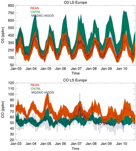
Fig. 5 Same as Fig. 2 for the UT.

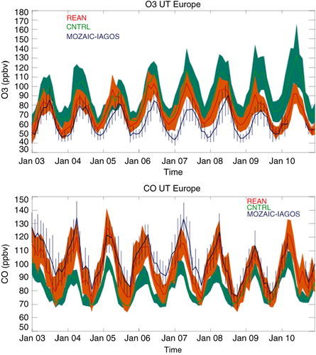
In the LS (Fig. 4), CNTRL tends to overestimate ozone by 100–200 ppbv, while CO is well reproduced with a MB close to zero. After assimilation, the model (REAN) tends to underestimate ozone by about (or less than) 50 ppbv on average during the period where MLS bias correction was applied (2005–2007) and by 70 ppbv on average outside this period. REAN tends to overestimate CO by 20 ppbv on average throughout the period.

In the LS, the seasonal cycle of ozone is well reproduced by the models but in most years, CNTRL overestimates the ozone spring/summer maximum by 150–200 ppbv, whereas REAN mostly underestimates the ozone spring/summer maximum by about 50 ppbv. For CO, a seasonal cycle is introduced via assimilation. Such a seasonal cycle is not observed by MOZAIC-IAGOS. This leads to positive biases around 20 ppbv for REAN on average, while the average biases are close to zero for CNTRL.

In the LS, it is worth noting that an overall maximum of CO is observed from April 2007 until August 2007. This maximum of CO is likely due to long range transport of anthropogenic emissions in spring and to transport of a CO plume into the Ex-UTLS during a strong episode of forest fires in early summer. This broad spring/summer anomaly of CO is not reproduced by the two models, although REAN captures the peak value well. According to Kaiser et al. (2012), the fire radiative energy (FRE) observed by MODIS shows a high value in 2007 in North America and in Europe compared with the other years. In Europe, this is also seen in GFAS inventory which uses FRE and is linked to strong fire emissions in Greece. However, the maximum of the emissions in 2007 is not seen in GFED inventory. As this was the inventory used in the REAN in 2007, the bias could be partly explained by the uncertainties of the fire emission inventory GFED.

In the UT (Fig. 5), CNTRL tends to overestimate ozone by up to 50 ppbv and to underestimate CO by around 40 ppbv. After assimilation (REAN), the bias in ozone decreases (overestimation by less than 30 ppbv), and the bias in CO changes sign (underestimation to overestimation by less than 20 ppbv).

In the UT, the seasonal cycle of ozone is well reproduced but the ozone spring/summer maximum is overestimated by both models. For CO, the spring/summer minimum is overestimated by both models but after 2008, when the assimilation of IASI is introduced, the biases of REAN decrease.

Figure 6 shows the difference of ozone and CO mixing ratios between LS and UT as a measure of the gradients around the tropopause. We note that the cross-tropopause difference in ozone mixing ratio has been changed after assimilation. This difference in ozone tends to be overestimated by CNTRL and mostly underestimated by REAN. For CO, the cross-tropopause difference has not been changed after assimilation and tends to be underestimated (by about 20 ppbv) in both CNTRL and REAN. Assimilation of stratospheric ozone profiles and ozone total columns leads to changes of ozone both in the stratosphere and the troposphere, whereas the assimilation of CO total columns has an impact on CO mostly in the troposphere, because of the sensitivity of the satellite data. MOPITT and IASI are sensitive to CO mainly between 300 and 700 hPa (Inness et al., 2013), whereas the band of the Ex-UTLS region, defined with MOZAIC-IAGOS, is between 200 and 300 hPa. As a result, tropospheric CO is corrected by the assimilation of data from these satellites (MB less negative in REAN than in CNTRL in the UT, as seen in Fig. 5), but the gradient around the tropopause remains unchanged (Fig. 6). Therefore, this leads to a significant positive biases of CO observed in the LS (Fig. 4) which is not offset by the stratospheric chemistry in the MOZART CTM.

Fig. 6 Time series of LS minus UT differences of ozone (top) and CO (bottom) monthly means.

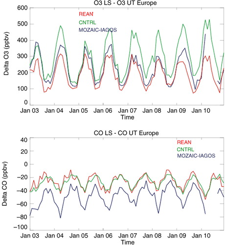
As a conclusion, REAN performs differently compared to CNTRL for ozone and CO in the Ex-UTLS, with a strong positive impact from the assimilation of ozone in the LS, but a less pronounced positive impact in the UT. For CO there is a strong positive impact in the troposphere, but a negative impact in the stratosphere over the whole period. Assimilation of stratospheric ozone profiles and ozone total column leads to changes of ozone both in the stratosphere and the troposphere. Therefore, the cross-tropopause difference in ozone mixing ratios decreases between CNTRL and REAN to become less than in the observations. As the effects of the assimilation of CO are felt in the mid-troposphere, the cross-tropopause difference of CO remains underestimated by the models.

4.1.2. Focus on phase and amplitude of seasonal cycles

This section gives a complementary evaluation of the ability of REAN to reproduce the seasonal cycle, in terms of amplitude and phase of the monthly means of the two model versions and the observations. The correlation coefficient R is used to test the agreement in phase of the seasonal cycle, the standard deviation s is used to quantify the amplitude of the seasonal cycle and the unbiased root mean square difference (RMSD′) is used to assess the global errors of the model to reproduce the seasonal cycle (see Section 3.2.2 and Taylor, 2001). Thus, these three statistical parameters give more information on the nature of the differences between the observations and models. They are presented in the Taylor diagrams in Fig. 7.

Fig. 7 Normalised Taylor diagrams for ozone (left) and CO (right) in the LS (top) and the UT (bottom) for both models REAN (red) and CNTRL (green), from 2003 to 2009. Years are referred in black (‘YY’) above each point. Point in blue (Obs) is the observation MOZAIC taken as the reference (R=1 and s=1). A perfect model would coincide with the observations at R=1, s=1. The minimum value for correlation in the figures is limited to zero, explaining missing data points in some cases.

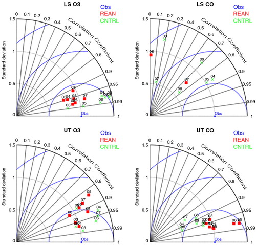
In the LS (top panels of Fig. 7), almost all standard deviations (σ) of CNTRL for ozone are greater than 1, whereas most s of REAN are lower than 1 (horizontal shift on the Taylor diagram after assimilation). It shows that assimilation tends to reduce the positive bias of the amplitude of the seasonal cycle of ozone. For CO, as shown in Section 4.1.1, the assimilation introduces a seasonal cycle which is not observed with MOZAIC-IAGOS. This is well summarised in the Taylor diagram as the unbiased root mean square difference (RMSD′) is greater than 1 for REAN (indeed not shown as outside the range of the plot).

In the UT (bottom panels of Fig. 7), the correlation coefficients (R) of CNTRL for ozone are mostly greater than 0.9, whereas R of REAN could be lower than 0.9 (vertical shift after assimilation). It shows that assimilation tends to increase the biases of the phase of the seasonal cycle of ozone. However, according to s values, the ability of the model to reproduce the amplitude of the seasonal cycle of ozone has been improved by the assimilation for some years (2004, 2006 and 2007). For CO, σ of CNTRL are lower than 1, whereas s of REAN are close to 1, most of the time. It shows that the assimilation tends to decrease the negative biases of the amplitude of the seasonal cycle of CO.

As a conclusion, the positive impact of the assimilation for ozone in the LS and for CO in the UT, as shown in Section 4.1.1 using MB, corresponds more to a better ability of the model to reproduce the amplitude of the seasonal cycle rather than its phase. The less pronounced impact of the assimilation for ozone in the UT corresponds more to the worsening of the seasonal cycle phase than the amplitude considering that the amplitude is actually better simulated most of the time after assimilation.

4.1.3. Focus on the changes over the 8-yr period

This section investigates the ability of the models to reproduce the observed inter-annual variability of ozone and CO between 2003 and 2009. 2010 is excluded as there is a lack of MOZAIC data between April and August, which could lead to important uncertainties in the comparison with the models. The objective is here to present a measure of the changes of ozone and CO over the period, to facilitate the comparison between observations and model outputs. In its current version, because of the changes in the assimilated datasets, REAN is not an appropriate run for a trend analysis. However, analysis of the temporal evolution of model/observations differences is of interest.

As a measure of these differences, we present and summarize the behaviours in terms of annual and seasonal anomalies as linear fits over the period 2003 to 2009.

The ozone and CO anomalies are obtained by removing the seasonal variability from ozone or CO mixing ratios.

Figure 8 shows the inter-annual variability of ozone and CO in terms of annual means of anomalies in the LS and the UT from 2003 to 2009 for both MACC model versions and MOZAIC-IAGOS data. The uncertainty of the trends results from the 2-sigma estimation of the fit parameters. The trend is considered statistically significant when the 2-sigma value is less than the slope of the fit.

Fig. 8 Time series of annual means (solid) and associated trends (dashed) as linear fit calculated from annual mean anomalies of ozone and CO in the LS (top) and the UT (bottom) for REAN (red), CNTRL (green) and MOZAIC/IAGOS observations (blue) from January 2003 to December 2009. Overall linear trends are also indicated on the figure for the three datasets. The 2-sigma values are given to assess the uncertainty of the trends. The black line corresponds to an anomaly equal to zero.

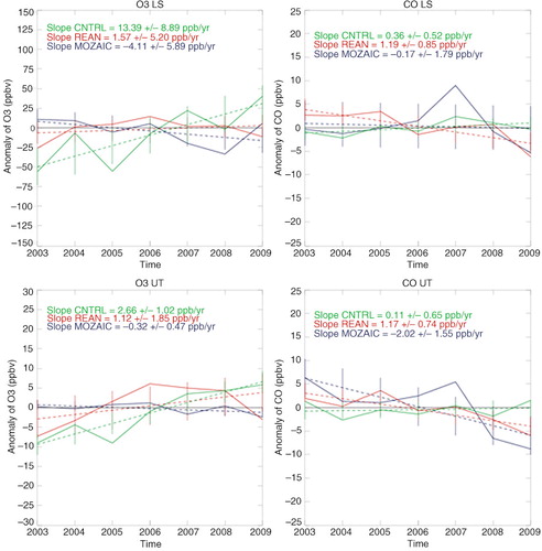
In the LS (top panels of Fig. 8), observations show a negative anomaly of ozone between −25 and −40 ppbv (~10–15%) in 2007 and 2008 and a positive anomaly of CO of about 10 ppbv (~10%) in 2007. This latter anomaly is due to the maxima of CO observed in spring/summer 2007 (Fig. 4). From Fig. 8, it is clear that there is no significant trend of ozone and CO between 2003 and 2009 observed by MOZAIC-IAGOS in the LS. REAN and CNTRL do not reproduce this observed inter-annual variability of ozone and CO in the LS. CNTRL produces a significant positive trend of ozone with +13.4±8.9 ppbv/yr, but REAN is closer to observations with no discernible trend. For CO, REAN produces a slightly negative trend (−1.2±0.9 ppbv/yr) and CNTRL is closer to observations of CO, as seen in Fig. 4. CO from REAN is too high at the beginning of the period, but the observed negative tendency observed after 2008 is well reproduced, even though the 2007 anomaly is missed.

In the UT (bottom panels of Fig. 8), there is no significant trend of ozone measured by MOZAIC-IAGOS and the annual anomalies of ozone are close to 0. This is in agreement with recent studies of the long-term trend of ozone in the free troposphere over Europe (Logan et al., 2012; Gaudel et al., 2015). For CO, observations show a positive anomaly in 2007 greater than 5 ppbv (> 5%, a bit less than in the LS) which is maximal in spring/summer (Fig. 5), and negative anomalies in 2008 and 2009 of about −5, −10 ppbv (5–10%). Despite the rather short time series, it is worth noting that a significant negative trend of CO of −2.0±1.6 ppbv/yr is observed in the UT between 2003 and 2009. Worden et al. (2013) have inferred, using total column CO measured by MOPITT, a decrease of CO of −3.03±0.46 (1σ error) molecules/cm²/year over Europe from 2000 to 2012. This observed decrease of CO could be related to the significant decrease of North American emissions (Granier et al., 2011) as the North American emissions has the most important influence on UT composition compare to European and (central and South-East) Asian emissions (Petetin et al., 2015).

In the UT, CNTRL produces a significant trend of ozone (2.7±1.0 ppbv/yr) which is not observed and CNTRL does not reproduce the decrease of CO. After assimilation (REAN), the model produces positive anomalies of ozone between 2005 and 2008 which are seen neither in the observations nor in CNTRL. The time-period 2005–2008 corresponds to the period of the MLS bias correction issue (see Section 2.2). For CO, REAN is able to reproduce the decrease observed in the UT with a trend of −1.2±0.7 ppbv/yr, of same order of magnitude as the observed one (−2.0 ppb/yr). In particular, negative anomalies of CO in 2008 and 2009, when IASI was assimilated in addition to MOPITT, are well reproduced. However, note that the positive anomaly in 2007 (also seen in the LS) is still not well reproduced by either REAN or CNTRL. This may be attributed to limitations in the use of the biomass burning inventory GFED (2003–2008) and limitations of the model to transport biomass burning plumes up to the Ex-UTLS region. Looking into seasonal changes over the period (not shown), it appears that the maximum of observed negative trends of CO are seen in winter (−2.7±2 ppbv/yr) when anthropogenic emissions maximise. REAN reproduces well the decrease of CO in winter (−2.6±1.9 ppbv/yr). This confirms the possible link with the reduction of anthropogenic emissions over North-Eastern America (Granier et al., 2011) as the transport from North-Eastern America toward Europe through the North Atlantic corridor and due to strong warm conveyor belt (WCB) (Stohl and Trickl, 1999; Cooper et al., 2002a, 2002b; Stohl et al., 2003), is maximal in winter. It illustrates also the ability of the model to represent the impact of the reduction of North American emissions included in the model through the MACCity anthropogenic emissions inventory. However, in spring/summer, the observed CO distribution and its inter-annual variability (as highlighted by the anomaly in 2007) are also driven by other sources (e.g. biomass burning from boreal latitudes or the Mediterranean region) along with specific transport processes, and in this season, the models perform less well. This seems to confirm the limitation of the models to represent correctly the impact of biomass burning emissions included in the model through GFED (2003–2008) and GFAS (from 2008) inventories, probably due to biases in reproducing their vertical transport.

4.2. Evaluation of mixing in the Ex-UTLS

The aim of this section is to assess the ability of the model to reproduce mixing in the Ex-UTLS over Europe. Schematically, in an O₃/CO scatter plot, the vertical branch is related to the stratospheric reservoir and the horizontal branch to the tropospheric reservoir with mixing between the two resulting in linear mixing lines (Hoor et al., 2002; Brioude et al., 2008). Mixing lines in the Ex-UTLS over Europe can be assessed with in situ MOZAIC-IAGOS data as the two species are measured simultaneously.

Figure 9 shows seasonal O₃–CO scatter plots in the Ex-UTLS with MOZAIC-IAGOS, the reanalysis (REAN, with assimilation) and the control run (CNTRL, without assimilation) for the entire period 2003–2010, over Europe. MOZAIC-IAGOS data have been averaged on a grid with the same horizontal resolution as the models (1.125°×1.125°) in order to allow for a fairer comparison. We have chosen seasonal ozone and CO thresholds to define three regions: ‘Low CO’, ‘Low O₃’ and the ‘Extra tropical Transition Layer’ (ExTL) (as defined by Gettelman et al., 2011) in between, as marked in Fig. 9. The ozone threshold is the seasonal mean value of ozone in UT and the CO threshold is the seasonal mean value of CO in LS. UT and LS refer to the two layers defined in Section 3.1.

Fig. 9 Seasonal PDF of ozone as a function of CO in the Ex-UTLS for MOZAIC-IAGOS data averaged in a grid with horizontal resolution of 1.125° × 1.125° (first column), REAN (second column) and CNTRL (third column). The shape of the PDF for MOZAIC-IAGOS is reproduced on the model panels in black and white. The black lines correspond to the limits of the ‘low CO’ region, the ‘low O₃’ region and the extra tropical transition layer (ExTL) using seasonal thresholds of ozone (mean value of ozone in UT) and CO (mean value of CO in LS) in ppbv (blue on the panels).

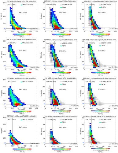
The mean values of ozone in UT (ozone threshold) calculated from MOZAIC-IAGOS data vary from 48/49 ppbv in winter/fall to 68/77 ppbv in spring/summer, whereas the mean values of CO in LS (CO threshold) vary from 50/48 ppbv in spring/summer to 52/51 ppbv in winter/fall. Thus the maximum of the ozone threshold is observed in summer but the maximum of the CO threshold is observed in winter. The seasonal variability for ozone in the UT is much greater than for CO in the LS (see Section 4.1.1).

The maximum of the PDF (>1.3%) from MOZAIC-IAGOS is observed across a range of 20–250 ppbv for ozone and a range of 40–130 ppbv for CO, in winter/fall; and across a range of 20–150 ppbv for ozone and a range of 90–140 ppbv or 70–120 ppbv for CO in spring/summer. For middle and low PDF (<1.1%), a CO mixing ratio greater than 100 ppbv may correspond to an ozone mixing ratio lower than 150 ppb in winter/fall and ozone mixing ratios greater than 300 ppbv in spring/summer, indicating that the ExTL has a greater depth in spring/summer.

In each season, the percentage of air classified as ‘low CO’ or ‘low ozone’ is about 20%, and about 60% of the data are classified in the ExTL region. The ExTL captures a maximum of 63% of the observations in summer when the depth of the ExTL is known to be at a maximum (Hoor et al., 2002).

The mean values of CO in LS (threshold of CO) are rather well reproduced by CNTRL (3rd column of Fig. 9) (around 50 ppbv with a maximum in winter), whereas the mean values of ozone in UT (threshold of ozone) are overestimated by 20 to 30 ppbv depending on season. CNTRL tends to overestimate the range of ozone and underestimate the range of CO for all values of PDF. In general, CNTRL does not reproduce the observed seasonal variability of the PDF distribution as it has underestimated the depth of the mixing layer particularly in spring/summer.

After assimilation (REAN: middle column of Fig. 9), the mean values of ozone in UT (ozone threshold) and the mean values of CO in LS (CO threshold), both become overestimated by the model with differences of 10–20 ppbv depending on season compared with the observations. After assimilation (REAN), the range of ozone for the high PDF (>1.3%, maximum of sampling) is still overestimated in spring/summer and becomes underestimated in winter, compared with CNTRL. For the distribution of CO for high PDF (> 1.3%, maximum of sampling), the model results get closer than the observation after assimilation. For middle and low PDF (<1.1%, minimum of sampling), the range of ozone is no longer overestimated after assimilation, but the range of CO is still underestimated and the model still misses the extreme values of CO.

The percentage of air classified as ‘Low CO’, ‘Low O₃’ and ‘Ex-TL’, shows differences after assimilation (REAN). The ‘Low O₃’ ratio is reduced by 10 to 15% compared with CNTRL and MOZAIC-IAGOS, depending on season, and the maximum of the ratio for the ExTL region has shifted from summer to spring compared with CNTRL and MOZAIC-IAGOS. Therefore in spring, when mixing is maximal, the ExTL ratio is overestimated by REAN, which is in agreement with other studies. Barré et al. (2013) showed that, although the location of the ExTL is improved by the assimilation of the satellite data (MLS and MOPITT in MOCAGE), the spread of the ExTL tends to be increased compared with a free-model run showing an overestimation of the mixing. It is worth noting that the differences between the thresholds between model and observations do not induce significant differences on percentage of air masses classified in the three regions ‘Low CO’, ‘Low O₃’ and ‘Ex-TL’ as they are equivalent to the percentages calculated with MOZAIC-IAGOS, except in spring.

As a consequence, the impact of assimilation on the O₃–CO correlation in the Ex-UTLS is definitely linked to the impact of the vertical distribution of the two species around the tropopause as we show in Figs. 10 and 11. Figures 10 and 11 show vertical distributions of ozone and CO, respectively, around the tropopause for the period 2003–2010. The pressure coordinate is relative to the pressure level of the dynamical tropopause. The two figures show that the threshold values of ozone and CO that we used to define the three regions in the UTLS are consistent with the mean profiles of ozone and CO. The observations and models have different threshold values which are directly related to the shape of the ozone and CO gradients which are not necessarily improved by the assimilation.

Fig. 10 Seasonal PDF of O₃ profile around the tropopause for the entire period 2003–2010 with pressure coordinate relative to the pressure level of the dynamical tropopause. As in Fig. 9, the first column is MOZAIC-IAGOS averaged in a grid with horizontal resolution of 1.125°×1.125°, the second column is REAN and the third column is CNTRL. The shape of the PDF for MOZAIC-IAGOS is reproduced on the model panels in black and white. Black lines correspond to mean profiles. GradS and GradT are the delta O₃ between 0 and 80 hPa above and below the dynamical tropopause.

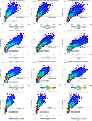
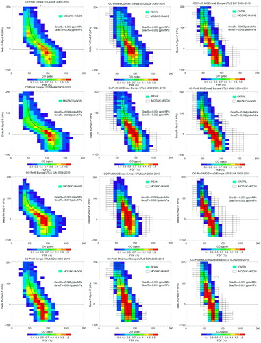
Fig. 11 Same as Fig. 10 for CO.

The ozone gradient above the dynamical tropopause is reduced after assimilation which induces an underestimation of the observed gradient by the models for the four seasons. After assimilation, the ozone gradient below the dynamical tropopause is also reduced after assimilation, decreasing the differences in the mean profile of ozone between the model and the observations. If we compare Fig. 10 with Figs. 4 and 5, the link between the changes on ozone gradients around the tropopause and on the ozone values in UT and LS due to assimilation is not obvious. Indeed, the decrease of the biases of ozone mixing ratios is more important in the LS than in the UT (Figs. 4 and 5) when the decrease of the differences in ozone gradients is more important in UT than in LS (Fig. 10).

Figure 11 highlights that the CO gradient around the tropopause does not change after assimilation. The observed negative CO gradient is still underestimated above the tropopause for the four seasons by REAN compared with CNTRL. The most noticeable changes after assimilation are the CO values in the column around the tropopause as they are shifted toward higher level of CO in both the UT and the LS. This explains the reduced biases in UT and the increase of these biases in LS as seen in Figs. 4 and 5. Furthermore, the small changes seen in the gradient of CO around the dynamical tropopause are in agreement with the results of Fig. 6. As noted in Section 3.1, the dynamical tropopause should not be different between observations and models as the PV field is based on the ECMWF operational model for all three data sets.

In conclusion, the shape of the O₃/CO scatter plot is quite well reproduced by the models. In general, REAN is doing a better job than CNTRL. Nevertheless, the models still have difficulties in properly reproducing the lowest and the highest CO mixing ratios and the mixing lines that are observed by dataset of MOZAIC-IAGOS, especially in spring/summer. This is directly linked to the ability or the inability of the models to reproduce the ozone and CO gradients (e.g. Clark et al., 2007). The CO gradient does not change significantly after assimilation. The weak vertical resolution of the models (500 m compared with 30 m for MOZAIC-IAGOS), the averaging kernel of MOPITT and IASI (CO measurement) applied to the MOZART-IFS system and background errors may limit the ability of REAN to reproduce the observed O₃–CO relationships in the Ex-UTLS (between 300 and 200 hPa, a 3 km-layer).

5. Conclusions

The MOZAIC-IAGOS programme provides high density and high resolution ozone and CO simultaneously recorded in-situ data. These data are used in this study to evaluate the MACC reanalysis (Inness et al., 2013) with the overall objective of assessing the ability of the model to reproduce the observed temporal and spatial variability of ozone and CO in the Ex-UTLS region. The impact of data assimilation was investigated by comparing the results from the MACC reanalysis to a control run without data assimilation for the years 2003–2010 focussing on Europe.

In general, the reanalysis is closer to the observations than the control run, which underlines the significantly positive impact of data assimilation. This is encouraging and gives room for further improvement of the description of ozone and CO in the Ex-UTLS.

Nevertheless, the assimilation leads to an overestimation of ozone in the UT and of CO in the LS. Although the cross-tropopause difference in the ozone mixing ratio is better reproduced after assimilation, the cross-tropopause difference in the CO mixing ratio remains unchanged and thus poorly reproduced by the MACC reanalysis. For CO, the relatively coarse vertical resolution (~500 m) and the vertical mixing overestimated in the Ex-UTLS, could not be offset by the data assimilation because the satellite data are more sensitive to the CO in the mid-troposphere. The MACC reanalysis tends to add variability of stratospheric ozone into the UT and tends to add the variability of tropospheric CO into the LS. These results indicate that the assimilation of the total column retrievals does not properly attribute the stratospheric and tropospheric contribution to the column.

Problems also remain in reproducing the observed inter-annual variability. Observed CO is clearly decreasing in the UT but the MACC reanalysis shows this behaviour only in winter. The observed decrease is likely the result of the reduced North American emissions. For other seasons, deficiencies in transport, mixing processes and also emissions during extreme events may be important factors. In spring/summer 2007 a positive anomaly of CO is observed in the Ex-UTLS with MOZAIC-IAGOS data but not reproduced by either of the two models. North American and European anthropogenic and fire emissions would have an important impact on CO mixing ratios over Europe for this period, which models may not be able to capture.

In the critical Ex-UTLS region, both REAN and CNTRL have difficulties in reproducing the wide range of ozone (20–700 ppb) and CO (20–150 ppb) mixing ratios. The reanalysis performs better than the control run in reproducing the mixing lines in the Ex-UTLS. However, models have difficulties in reproducing low CO in LS and high CO in UT. This is directly linked to the fact that the ozone and CO gradients around the tropopause are not necessarily better reproduced by the model after assimilation. This illustrates the limitations of the current data assimilation system, and at the same time the impact of the coarse resolution in the Ex-UTLS region.

Finally, MOZAIC-IAGOS is an on-going programme providing regular data of reactive gases (and soon aerosols and greenhouse gases). Its long-term participation in CAMS will allow us to pursue such evaluations in the future and help the understanding and quantification of the processes playing a role in the Ex-UTLS region.

6. Acknowledgements

The authors acknowledge the strong support of the European Commission, Airbus, and the Airlines (Lufthansa, Air-France, Austrian, Air Namibia, Cathay Pacific, Iberia and China Airlines so far) who carry the MOZAIC or IAGOS equipment and perform the maintenance since 1994. MOZAIC is presently funded by INSU-CNRS (France), Météo-France, Université Paul Sabatier (Toulouse, France) and Research Center Jülich (FZJ, Jülich, Germany). IAGOS has been and is additionally funded by the EU projects IAGOS-DS, IAGOS-ERI, and IGAS. The MOZAIC-IAGOS database is supported by ETHER (CNES and INSU-CNRS).

MACC-II was funded by the European Commission under the EU Seventh Research Framework Programme, contract number 283576. The research leading to these results has received funding from the European Community's Horizon 2020 Programme under grant agreement n° 633080.

Notes

This paper is part of a Special Issue on MOZAIC-IAGOS in Tellus B celebrating 20 years of an ongoing air chemistry climate research measurement from airbus commercial aircraft operated by an international consortium of countries. More papers from this issue can be found at http://www.tellusb.net

References

- Aghedo A., Bowman K., Worden H., Kulawik S., Shindell D., co-authors. The vertical distribution of ozone instantaneous radiative forcing from satellite and chemistry climate models. . Geophys. Res. Atmos. 2011; 116(D01305): DOI: http://dx.doi.org/10.1029/2010JD014243.
- Barré J. , Amraoui L. E. , Ricaud P. , Lahoz W. , Attié J.-L. , co-authors . Diagnosing the transition layer at extratropical latitudes using MLS O3 and MOPITT CO analyses. Atmos. Chem. Phys. 2013; 13(14): 7225–7240.
- Bethan S. , Vaughan G. , Reid S. J . A comparison of ozone and thermal tropopause heights and the impact of tropopause definition on quantifying the ozone content of the troposphere. Q. J. Roy. Meteorol. Soc. 1996; 122(532): 929–944.
- Brioude J. , Cammas J. P. , Cooper O. R. , Nedelec P . Characterization of the composition, structure and seasonal variation of the mixing layer above the extratropical tropopause as revealed by MOZAIC measurements. J. Geophys. Res. 2008; 113(D7): 2156–2202.
- Clark H. , Cathala M.-L. , Teyssédre H. , Cammas J.-P. , Peuch V.-H . Cross-tropopause fluxes of ozone using assimilation of MOZAIC measurements in a global CTM. Tellus B. 2007; 59: 39–49.
- Cooper O., Moody J., Parrish D., Trainer M., Ryerson T., co-authors. Trace gas composition of midlatitude cyclones over the western North Atlantic Ocean: a conceptual model. J. Geophys. Res. 2002a.; 107 DOI: http://dx.doi.org/10.1029/2001JD000902.
- Cooper O. R., Moody J. L., Parrish D. D., Trainer M., Holloway J. S., co-authors. Trace gas composition of midlatitude cyclones over the western North Atlantic Ocean: a seasonal comparison of O3 and CO. J. Geophys. Res. 2002b; 107 DOI: http://dx.doi.org/10.1029/2001JD000901.
- Crutzen P. J . Photochemical reactions initiated by and influencing ozone in unpolluted tropospheric air. Tellus. 1974; 26(1–2): 47–57.
- Dee D. P. , Uppala S. M. , Simmons A. J. , Berrisford P. , Poli P. , co-authors . The ERA-Interim reanalysis: configuration and performance of the data assimilation system. Q. J. Roy. Meteorol. Soc. 2011; 137: 553–597.
- Derwent R. , Jenkin M. , Saunders S . Photochemical ozone creation potentials for a large number of reactive hydrocarbons under European conditions. Atmos. Environ. 1996; 30(2): 181–199.
- Edwards D. , Halvorson C. , Gille J . Radiative transfer modeling for the EOS Terra satellite Measurement of Pollution in the Troposphere (MOPITT) instrument. J. Geophys. Res. Atmos. 1999; 104(D14): 16755–16775.
- Elguindi N. , Clark H. , Ordoñez C. , Thouret V. , Flemming J. , co-authors . Current status of the ability of the GEMS/MACC models to reproduce the tropospheric CO vertical distribution as measured by MOZAIC. Geosci. Model Dev. 2010; 3(2): 501–518.
- Eskes H. , Huijnen V. , Arola A. , Benedictow A. , Blechschmidt A.-M. , co-authors . Validation of reactive gases and aerosols in the MACC global analysis and forecast system. Geosci. Model Dev. Discuss. 2015; 8: 1117–1169.
- Fischer H. , Wienhold F. , Hoor P. , Bujok O. , Schiller C. , co-authors . Tracer correlations in the northern high latitude lowermost stratosphere: influence of cross-tropopause mass exchange. Geophys. Res. Lett. 2000; 27(1): 97–100.
- Fishman J. , Watson C. E. , Larsen J. C. , Logan J. A . Distribution of tropospheric ozone determined from satellite data. J. Geophys. Res. Atmos. 1990; 95(D4): 3599–3617.
- Flemming J. , Inness A. , Flentje H. , Huijnen V. , Moinat P. , co-authors . Coupling global chemistry transport models to ECMWF's integrated forecast system. Geosci. Model Dev. 2009; 2: 253–265.
- Forster F. , Piers M. , Shine K. P . Radiative forcing and temperature trends from stratospheric ozone changes. J. Geophys. Res. Atmos. 1997; 102(D9): 10841–10855.
- Gaudel A. , Ancellet G. , Godin-Beekmann S . Analysis of 20 years of tropospheric ozone vertical profiles by lidar and ECC at Observatoire de Haute Provence (OHP) at 44°N, 6.7°E. Atmos. Environ. 2015; 113: 78–89.
- Gettelman A., Hoor P., Pan L., Randel W., Hegglin M., co-authors. The extratropical upper troposphere and lower stratosphere. Rev. Geophys. 2011; 49(3): RG3003. DOI: http://dx.doi.org/10.1029/2011RG000355.
- Granier C. , Bessagnet B. , Bond T. , D’Angiola A. , Van Der Gon H. D. , co-authors . Evolution of anthropogenic and biomass burning emissions of air pollutants at global and regional scales during the 1980–2010 period. Clim. Change. 2011; 109(1–2): 163–190.
- Guenther A. , Karl T. , Harley P. , Wiedinmyer C. , Palmer P. I. , co-authors . Estimates of global terrestrial isoprene emissions using MEGAN (Model of Emissions of Gases and Aerosols from Nature). Atmos. Chem. Phys. 2006; 6: 3181–3210.
- Hollingsworth A. , Engelen R. J. , Textor C. , Benedetti A , Boucher O. , co-authors . Toward a monitoring and forecasting system for atmospheric composition: the GEMS project. Bull. Am. Meteorol. Soc. 2008; 89(8): 1147–1164.
- Holton J. , Haynes P. , McIntyre M. , Douglass A. , Rood R. , co-authors . Stratosphere–troposphere exchange. Rev. Geophys. 1995; 33(4): 403–439.
- Hoor P., Fischer H., Lange L., Lelieveld J., Brunner D. Seasonal variations of a mixing layer in the lowermost stratosphere as identified by the CO–O3 correlation from in situ measurements. J. Geophys. Res. Atmos. 2002; 107(D5): 4044. DOI: http://dx.doi.org/10.1029/2000JD000289.
- Hoor P. , Gurk C. , Brunner D. , Hegglin M. , Wernli H. , co-authors . Seasonality and extent of extratropical TST derived from in-situ CO measurements during SPURT. Atmos. Chem. Phys. 2004; 4: 1427–1442.
- Inness A. , Baier F. , Benedetti A. , Bouarar I. , Chabrillat S. , co-authors . The MACC reanalysis: an 8 yr data set of atmospheric composition. Atmos. Chem. Phys. 2013; 13: 4073–4109.
- IPCC. Climate Change 2013: The Physical Science Basis. Contribution of Working Group I to the Fifth Assessment Report of the Intergovernmental Panel on Climate Change. 2013; Cambridge, United Kingdom: Cambridge University Press.
- Jolliff J. K. , Kindle J. C. , Shulman I. , Penta B. , Friedrichs M. A. , co-authors . Summary diagrams for coupled hydrodynamic-ecosystem model skill assessment. J. Mar. Syst. 2009; 76(1): 64–82.
- Kaiser J. W. , Heil A. , Andreae M. O. , Benedetti A. , Chubarova N. , co-authors . Biomass burning emissions estimated with a global fire assimilation system based on observed fire radiative power. Biogeosciences. 2012; 9(1): 527–554.
- Kanakidou M. , Dentener F. J. , Brasseur G. P. , Berntsen T. K. , Collins W. J. , co-authors . 3-D global simulations of tropospheric CO distributions – results of the GIM/IGAC intercomparison 1997 exercise. Chemosphere-Global Change Sci. 1999; 1(1): 263–282.
- Katragkou E. , Zanis P. , Tsikerdekis A. , Kapsomenakis J. , Melas D. , co-authors . Evaluation of near surface ozone over Europe from the MACC reanalysis. Geosci. Model Dev. Discuss. 2015; 8: 1077–1115.
- Kinnison D. E., Brasseur G. P., Walters S., Garcia R. R., Marsh D. R., co-authors. Sensitivity of chemical tracers to meteorological parameters in the MOZART-3 chemical transport model. J. Geophys. Res. Atmos. 2007; 112(D20): D20302. DOI: http://dx.doi.org/10.1029/2006JD007879.
- Logan J. A . Tropospheric ozone: seasonal behavior, trends, and anthropogenic influence. J. Geophys. Res. 1985; 90(D6): 10463–10482.
- Logan J. A., Staehelin J., Megretskaia I. A., Cammas J. P., Thouret V., co-authors. Changes in ozone over Europe: analysis of ozone measurements from sondes, regular aircraft (MOZAIC) and alpine surface sites. J. Geophys. Res. Atmos. 2012; 117(D9): D09301. DOI: http://dx.doi.org/10.1029/2011JD016952.
- Marenco A. , Thouret V. , Nédélec P. , Smit H. , Helten M. , co-authors . Measurement of ozone and water vapor by Airbus in-service aircraft: the MOZAIC airborne program, an overview. J. Geophys. Res. Atmos. 1998; 103(D19): 25631–25642.
- Naik V. , Voulgarakis A. , Fiore A. , Horowitz L. , Lamarque J.-F. , co-authors . Preindustrial to present-day changes in tropospheric hydroxyl radical and methane lifetime from the Atmospheric Chemistry and Climate Model Intercomparison Project (ACCMIP). Atmos. Chem. Phys. 2013; 13(10): 5277–5298.
- Nédélec P., Blot R., Boulanger D., Athier G., Cousin J.-M., co-authors. Instrumentation on commercial aircraft for monitoring the atmospheric composition on a global scale: the IAGOS system, technical overview of ozone and carbon monoxide measurements. Tellus B. 2015; 67 27791. DOI: http://dx.doi.org/10.3402/tellusb.v67.27791.
- Nédélec P. , Cammas J.-P. , Thouret V. , Athier G. , Cousin J.-M. , co-authors . An improved infrared carbon monoxide analyser for routine measurements aboard commercial Airbus aircraft: technical validation and first scientific results of the MOZAIC III programme. Atmos. Chem. Phys. 2003; 3: 1551–1564.
- Novelli P. , Masarie K. , Lang P. , Hall B. , Myers R. , co-authors . Reanalysis of tropospheric CO trends: effects of the 1997–1998 wildfires. J. Geophys. Res. Atmos. 2003; 108(D15): 4464.
- Ordoñez C. , Elguindi N. , Stein O. , Huijnen V. , Flemming J. , co-authors . Global model simulations of air pollution during the 2003 European heat wave. Atmos. Chem Phys. 2010; 10(2): 789–815.
- Pan L., Randel W., Gary B., Mahoney M., Hintsa E. Definitions and sharpness of the extratropical tropopause: a trace gas perspective. J. Geophys. Res. 2004; 109(D23103): DOI: http://dx.doi.org/10.1029/2004JD004982.
- Pan L. L., Bowman K. P., Shapiro M., Randel W. J., Gao R. S., co-authors. Chemical behavior of the tropopause observed during the Stratosphere-Troposphere Analyses of Regional Transport experiment. J. Geophys. Res. Atmos. 2007a; 112(D18): D18110. DOI: http://dx.doi.org/10.1029/2007JD008645.
- Pan L. L., Wei J. C., Kinnison D. E., Garcia R. R., Wuebbles D. J., co-authors. A set of diagnostics for evaluating chemistry-climate models in the extratropical tropopause region. J. Geophys. Res. Atmos. 2007b; 112(D9): D09316. DOI: http://dx.doi.org/10.1029/2006JD007792.
- Petetin H. , Thouret V. , Fontaine A. , Sauvage B. , Athier G. , co-authors . Characterizing tropospheric ozone and CO around Frankfurt between 1994–2012 based on MOZAIC-IAGOS aircraft measurements. Atm. Chem. and Phys. Discuss. 2015; 15: 23841–23891.
- Petzold A., Thouret V., Gerbig C., Zahn A., Brenninkmeijer C., co-authors. Global-scale atmosphere monitoring by in-service aircraft – current achievements and future prospects of the European research infrastructure IAGOS. Tellus B. 2015; 67 28452. DOI: http://dx.doi.org/10.3402/tellusb.v67.28452.
- Riese M., Ploeger F., Rap A., Vogel B., Konopka P., co-authors. Impact of uncertainties in atmospheric mixing on simulated UTLS composition and related radiative effects. J. Geophys. Res. Atmos. 2012; 117(D16): D16305. DOI: http://dx.doi.org/10.1029/2012JD017751.
- Schmidt T., Cammas J.-P., Smit H., Heise S., Wickert J., co-authors. Observational characteristics of the tropopause inversion layer derived from CHAMP/GRACE radio occultations and MOZAIC aircraft data. J. Geophys. Res. Atmos. 2010; 115(D24): D24304. DOI: http://dx.doi.org/10.1029/2010JD014284.
- Shindell D. T., Faluvegi G., Stevenson D. S., Krol M. C., Emmons L. K., co-authors. Multimodel simulations of carbon monoxide: comparison with observations and projected near-future changes. J. Geophys. Res. Atmos. 2006a; 111(D19): D19306. DOI: http://dx.doi.org/10.1029/2006JD007100.
- Stein O. , Flemming J. , Inness A. , Kaiser J. W. , Schultz M. G. . Global reactive gases forecasts and reanalysis in the MACC project. J. Integr. Environ. Sci. 2012; 9: 57–70.
- Stein O. , Schultz M. G. , Bouarar I. , Clark H. , Huijnen V. , co-authors . On the wintertime low bias of Northern Hemisphere carbon monoxide in global model studies. Atmos. Chem. Phys. Discuss. 2014; 14(1): 245–301.
- Stevenson D. S. , Young P. J. , Naik V. , Lamarque J. F. , Shindell D. T. , co-authors . Tropospheric ozone changes, radiative forcing and attribution to emissions in the Atmospheric Chemistry and Climate Model Intercomparison Project (ACCMIP). Atmos. Chem. Phys. 2013; 13(6): 3063–3085.
- Stohl A., Forster C., Eckhardt S., Spichtinger N., Huntrieser H., co-authors. A backward modeling study of intercontinental pollution transport using aircraft measurements. J. Geophys. Res. 2003; 108(D12): 4370. DOI: http://dx.doi.org/10.1029/2002JD002862.
- Stohl A. , Forster C. , Frank A. , Seibert P. , Wotawa G . The Lagrangian particle dispersion model FLEXPART version 6.2. Atmos. Chem. Phys. 2005; 5: 2461–2474.
- Stohl A. , Trickl T . A textbook example of long-range transport: simultaneous observation of ozone maxima of stratospheric and North American origin in the free troposphere over Europe. J. Geophys. Res. 1999; 104(D23): 30445–30462.
- Taylor K. E . Summarizing multiple aspects of model performance in a single diagram. J. Geophys. Res. Atmos. 2001; 106(D7): 7183–7192.
- Thouret V. , Cammas J. P. , Sauvage B. , Athier G. , Zbinden R. , co-authors . Tropopause referenced ozone climatology and inter-annual variability (1994–2003) from the MOZAIC programme. Atmos. Chem. Phys. 2006; 6(4): 1033–1051.
- Thouret V. , Marenco A. , Logan J. A. , Nédélec P. , Grouhel C. , co-authors . Comparisons of ozone measurements from the MOZAIC airborne program and the ozone sounding network at eight locations. J. Geophys. Res. Atmos. 1998; 103(D19): 25695–25720.
- Tilmes S., Pan L. L., Hoor P., Atlas E., Avery M. A., co-authors. An aircraft-based upper troposphere lower stratosphere O3, CO, and H2O climatology for the Northern Hemisphere. Geophys. Res. Atmos. 2010; 115(D14): D14303. DOI: http://dx.doi.org/10.1029/2009JD012731.
- Van der Werf G. R. , Randerson J. T. , Giglio L. , Collatz G. J. , Mu M. , co-authors . Global fire emissions and the contribution of deforestation, savanna, forest, agricultural, and peat fires (1997–2009). Atmos. Chem. Phys. 2010; 10(23): 11707–11735.
- WMO. Weather and Climate – Understanding risks and preparing for variability and extremes. Bulletin – The journal of the World Meteorological Organization. 2014; 63(2): Online at: https://2a9e94bc607930c3d739becc3293b562f744406b.googledrive.com/host/0BwdvoC9AeWjUazhkNTdXRXUzOEU/bulletin_63-2_en.pdf.
- Worden H. M. , Deeter M. N. , Frankenberg C. , George M. , Nichitiu F. , co-authors . Decadal record of satellite carbon monoxide observations. Atmos. Chem. Phys. 2013; 13(2): 837–850.
- Wotawa G. , Novelli P. , Trainer M. , Granier C . Inter-annual variability of summertime CO concentrations in the Northern Hemisphere explained by boreal forest fires in North America and Russia. Geophys. Res. Lett. 2001; 28(24): 4575–4578.
- Zahn A., Brenninkmeijer C., Asman W., Crutzen P., Heinrich G., co-authors. Budgets of O3 and CO in the upper troposphere: CARIBIC passenger aircraft results 1997–2001. J. Geophys. Res. 2002; 107(D17): 4337. DOI: http://dx.doi.org/10.1029/2001JD001529.
- Zahn A. , Brenninkmeijer C. , Maiss M. , Scharffe D. , Crutzen P. , co-authors . Identification of extratropical two-way troposphere-stratosphere mixing based on CARIBIC measurements of O3, CO, and ultrafine particles. J. Geophys. Res. 2000; 105(D1): 1527–1535.