Abstract
Due to a significant decrease in the cost of DNA sequencing, the number of sequences submitted to the public databases has dramatically increased in recent years. Efficient analysis of these data sets may lead to a significant understanding of the nature of pathogens such as bacteria, viruses, parasites, etc. However, this has raised questions about the efficacy of currently available algorithms for the study of pathogen evolution and construction of phylogenetic trees. While the advanced algorithms and corresponding programs are being developed, it is crucial to optimize the available ones in order to cope with the current need. The protocol presented in this study is optimized using a number of strategies currently being proposed for handling large-scale DNA sequence data sets, and offers a highly efficacious and accurate method for computing phylogenetic trees with limited computer resources. The protocol may take up to 36 h for construction and annotation of a final tree of about 20,000 sequences.
Introduction
An understanding of the genomic material of any living organism is indispensable for investigation of not only the genetic nature but also the origin of these organisms. Current advances in DNA sequencing have changed the scientific horizon, and greatly enhanced our knowledge about the genetic makeup of all pathogens including viruses, bacteria, parasites, etc. Moreover, these advances have made the application of genetic engineering possible toward an era of synthetic designs of several microorganisms, such as infectious clones for viruses. A thorough deciphering of the genetic sequences of these organisms will shed light on novel biological functions and phenotypic differences, which ultimately can be exploited in the service of humanity.
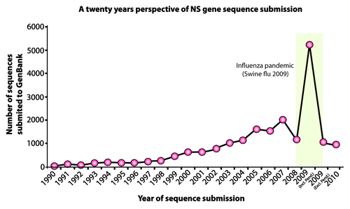
With a significant decrease in the cost of DNA sequencing, the number of sequences submitted to the public databases has dramatically increased in recent years. Furthermore, the increasing success of next generation sequencing technologies such as 454, Illumina and SOLiD, has revolutionized the availability of data on the genomic nature of all organisms including human and microorganisms.Citation1 As a result of this, many data sets have now increased in size exponentially and involve several hundred taxa in each organism. For instance, the number of sequences increased from 35,369 (in 2000) to 199,984 (in 2012) in 11 years in influenza A viruses alone (Influenza Research Database), and a similar trend has occurred for all other potential pathogens.
The availability of this huge amount of data are indeed a worthwhile resource; however, it challenges scientists to place this information in a biologically meaningful context, which usually is achieved by structuring the data in terms of evolutionary relationships as shown in a phylogenetic tree. This raises questions about the efficacy of the currently available algorithms for the study of pathogen evolution and the construction of phylogenetic trees. The currently available evolution models,Citation2,Citation3 especially those models that include rate variation among sites,Citation4-Citation6 require an increasing amount of calculation. Moreover, the algorithms conventionally applied to build phylogenetic trees often become overwhelmed as the number of sequences for analysis increases, resulting in reduced accuracy of tree structure and absurdly long computation times. The implementation of new or modified algorithms for handling large sequence data sets is paramount to our understanding of evolutionary processes in genomes and gene sequences. The protocol presented in this study is optimized using a number of strategies currently being proposed for handling large-scale DNA sequence data sets, and offers a highly efficacious and accurate method for computing phylogenetic trees, especially with limited computer resources.
Materials
Equipment
(1) MacOSX computer with minimum 2.4 GHz processor and 2 GB RAM.
(2) TextEdit or TextWrangler.
(3) CodonCode Aligner—DNA Sequence Assembly, Alignment and Editing.
(4) A Perl script for generating suitable file formats.
(5) RAxML BlackBox or RAxMLGUI.
(6) FigTree v1.2.3.
Equipment Set Up
MacOSX, an operating system
Throughout this protocol, MacOSX as an operating system is used and only software compatible with this system has been selected and optimized. However, with suitable modifications the same protocol can equally be applied for Windows. The MacBookPro with 2.4 GHz processor and 2 GB RAM, which is the least power of such computers, is sufficient to analyze a data set of minimum 20,000 sequences (tested in this protocol). However, the more processing capacity and internal memory available, then less time will be required to finish the jobs.
TextEdit or TextWrangler
TextEdit is a small tool that is available in MacOSX as the default program and is equivalent to WordPad in Windows. TextWrangler is another capable text editor for Mac users, which is freely available to download at the Bare Bone Website (www.barebones.com/products/TextWrangler/download.html). Either of these can be used to view the data sets, to carry out necessary editing, and to remove ambiguous or illegal symbols from the data sets.
CodonCode Aligner
CodonCode Aligner is a program for sequence assembly, alignments, contig editing and detecting mutation features, while offering a familiar, easy-to-learn user interface, and is available for Windows and MacOSX.Citation7 Because CodonCode Aligner is not an open access program, alternative tools such MUSCLE can also be used as a suitable alternative. In some situations, ClustalW may also be used. However for larger data sets, as in this protocol, CodonCode Aligner appears to be very fast, and is available for a 30-d fully functional trial at www.codoncode.com/aligner/. The major advantages of the CodonCode Aligner include end clipping, sequence assembly, alignment and option to select reference sequence without having to install a separate program. However, it is not an open access program, which may restrict its use to some of the researchers with limited funding.
Generating suitable file formats
One of the critical issues in handling larger data sets is the efficient maintenance of the sequence names. In the default setting for many of the programs, only the initial ten characters are maintained in the sequence name (as they use the Phylip format), which makes it difficult to label and interpret the results in an annotated phylogenetic tree. Therefore, a Perl script is used to convert Fasta sequences into Phylip format while keeping the complete sequence names. Use of this script is not only helpful for conversion of the formats in a quick way, but is also an easy and neat method that doesn’t incorporate any errors. Moreover, most of the available programs and tools for handling larger data sets require Phylip format for the sequences of interest.
RAxML (Randomized Axelerated Maximum Likelihood) BlackBox or RAxMLGUI
Once a data set with suitable sequence names (with the required information) and format (Phylip) is ready, it can be used for the construction of a phylogenetic tree in either RAxML BlackBox or RAxMLGUI. The RAxML BlackBox is a rapid bootstrap algorithm for the RAxML Web Servers, and the service is freely available at http://phylobench.vital-it.ch/raxml-bb/index.php. Alternatively, a user-friendly interface (RAxMLGUI) for the same algorithm can be downloaded freely from https://sites.google.com/site/raxmlgui/ and can be installed on several operating systems. RAxML is a program for sequential and parallel Maximum Likelihood-based inference of large phylogenetic trees. Within RAxML, several heuristics approaches are applied to maximally reduce the search time.Citation8 Initially, a starting tree under parsimony using random stepwise addition is built followed by branch swapping by using Lazy Subtree Rearrangements. The use of GTR + CAT, instead of GTR + GAMMA, contributes to the handling of larger taxa. Finally, a simulated annealing is used, which incorporates a cooling schedule and allows “backward steps” during the hill-climbing process. In addition to RAxML, for estimation of maximum-likelihood (ML) phylogenies, PhyML 3.0 can be freely accessed at www.atgc-montpellier.fr/phyml/, which is a suitable alternative to RAxMLGUI for fast and accurate construction of trees. The major drawback of the RAxML is the initial rearrangement setting, which might be very high (e.g., 20 or 25) and the program will slow down considerably. This requires restart of the program.
FigTree v1.2.3 and parallel software
Any of the programs capable of displaying large phylogenies can be used, such as Archaeopteryx (www.phylosoft.org/archaeopteryx/), Dendroscope (http://ab.inf.uni-tuebingen.de/software/dendroscope/), Jstree (http://lh3lh3.users.sourceforge.net/jstree.shtml) or PhyloWidget (www.phylowidget.org). However, FigTree (http://tree.bio.ed.ac.uk/software/figtree/) was found to be the most convenient program for handling larger trees, and is therefore used in this protocol.
Procedures
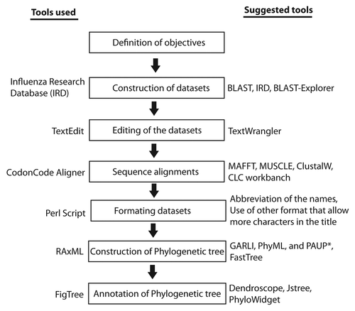
Different tools and packages were applied to find the best possible combination of programs that facilitates the user-friendly computation and refinement of trees, especially when a phylogenetic tree consists of thousands of taxa. All of these components are incorporated into the complete protocol, which is described here, step by step and is outlined in .
Figure 1. An illustration outlining the procedure demonstrated in this protocol. All the tools used in this protocol are mentioned on the left side whereas the tools that can be used in future are mentioned on the right side of the figure.
(1) Defining objectives
Different biologists may be concerned about getting different outputs from same phylogenetic analysis. Failing to create a proper objective can lead to drawing incorrect conclusions from phylogenetic studies. It is therefore essential to define the objective for the downstream analyses. The objective of analyzing the data set presented in this protocol was to estimate the distribution pattern of non-structural gene 1 (NS1) in different clades of the avian influenza A virus from 1902–2012 (). Moreover, it was in mind to evaluate the use of NS1 gene as “marker of evolution” for influenza viruses.
(2) Construction of data sets
Since there are different interpretations of the same phylogenetic tree, there is no single way for constructing data sets suitable for phylogenetic analysis. However, clarity while setting the objective will greatly help in constructing better data sets. Tools have been specifically designed to distinguish between orthology and paralogy in genome/proteome data setsCitation9 and expressed sequence tag data setsCitation10,Citation11 but they not always the most convenient for punctual analyses. The most common interest of most researchers is to compare the query sequence to that of sequences available in GenBank, and to extract the sequences in order to create a data set for subsequent construction of a phylogenetic tree. The Basic Local Alignment Search Tool (BLAST)Citation12 is the most widely used tool for this purpose, primarily owing to its speed of execution. However, the data extracted from BLAST is not always optimized and suitable for downstream phylogenetic analysis. Moreover, the order of BLAST hits does not reflect the evolutionary distances between the query and matching sequences. To address the shortcoming of BLAST tool, BLAST-Explorer (available at www.phylogeny.fr) provides a simple, intuitive and interactive graphical representation of the BLAST results, and allows selection and retrieval of the BLAST hit sequences based on a wide range of criteria. Notably, BLAST-Explorer is primarily aimed at helping the construction of sequence data sets for further phylogenetic study, and it can also be used as a standard BLAST server with enriched output.
In this protocol, the Influenza Research Database (IRD) has been used to exemplify the construction of data sets. The IRD has the primary aim to facilitate an understanding of the influenza virus and how it interacts with the host organism, leading to new treatments and preventive actions. To construct a data set using IRD, follow these steps:
• Go to the IRD webpage: www.fludb.org/brc/home.do?decorator=influenza
• Then click on the “Nucleotide Sequences” in the “Search Sequence” under the main tab “SEARCH DATA.”
• Depending upon the question in mind, one can choose an appropriate database. In this example “Segment data” in the “Sequence & Stains” was chosen.
• Set the following parameters before searching: Segment/Nucleotide under DATA TO RETURN, A under VIRUS TYPE, NS1/NS2 under SELECT SEGMENTS, All under HOST and GEOGRAPHIC GROUPING. !CAUTION It is possible to exclude any gene that belongs to the 2009 pandemic to avoid oversaturation of identical sequences. To further specify the required analysis, follow the option in “ADVANCED OPTIONS.”
• After setting the above parameters, the search will return 20,341 segments that span over 100 years and can be displayed on 407 pages (if 50 sequences per page).
• Click on the “Download” after checking “Select all 20,341 segments” and choose “Segment FASTA” among “Download Options” !CAUTION It is possible to save this search for later use or to save the search in a personal “Working Set.” For the latter option, a free log-on service is available. It is also important to assign a unique name to this newly downloaded data set. One can do so in the “Download Options.” For the sake of clarity, the data set was named “AllNSGenes” which is used throughout this protocol (Sup. Material 1).
• Either save the TICKET NUMBER, which appears in the download window, or wait for the download of the data set based on your default download setting.
(3) Editing of the data sets
It is crucial to edit the data sets to remove any illegal characters (see below) and harmonize the sequence names. This is of special concern when sequences are downloaded directly from GenBank, because sequence names may have all of the information but it may be disordered. To avoid complications in downstream analyses, edit the data set as described below:
• Open “AllNSGenes” data set (Sup. Material 1) with TextEdit.
• Remove identical names from the sequence names to avoid unnecessary extension of the sequence names. For example, gb:, Organism:, Influenza A virus, |Segment:8, |Subtype: and |Host: are present in all of the sequences and can be removed without losing any significant information. To do so, use the “Find” and “Replace with” options in the TextEdit, which can be popped up with “cmd+F” command in MacOSX. !CAUTION Keep in mind not to remove any of the greater than signs (>), which will destroy the Fasta format and may require rebuilding of the data set.
• It is also necessary to remove the illegal characters, mainly the pipeline sign (|), colon (:), semicolon (;) slash/stroke/solidus (/), apostrophe (’ '), quotation marks (‘ ’, “ ,” ' ', ” “), and brackets ([ ], (), { }, < >), among others. These characters can also be removed as described in the point above. !CAUTION It is important to replace these repetitive and illegal characters with the underscore/understrike (_) symbol. Remember not to replace any character with a similar symbol such as a dash (‒, –, —, —), which can create severe complications in the following analyses.
• It is of extreme important not to leave any “space” throughout the name of the sequence. If it exists, replace with an underscore (_) by using the “Find” and “Replace with” options in the TextEdit. This is crucial because CodonCode Aligner will only choose the sequence name until the first space, which leads to loss of most of the information in the sequence name and subsequently in the tree annotation. !CAUTION Don’t forget to save the changes in the data set before closing the file.
(4) Alignment of the sequences
Alignment can be performed with any program, algorithm, or tool available; however it must be able to handle large data sets, and must be fast and accurate. In my personal opinion, CodonCode Aligner has all of these features, and therefore is used in this analysis, as described below:
• Launch “CodonCode Aligner” after downloading and installation.
• Open the “AllNSGenes” data set by choosing “Open” in the “File” in the main bar. Expand the “Unassembled Samples.”
• Note the addition of all sequences (n = 20341) and that there is the full name of each sequence in the “Name” column. !CAUTION There may be some sequences of which the name may not contain the full name, which can be seen in the “Comments” column. If this happens, re-open the “AllNSGenes” data set in TextEdit and remove any spaces in the name.
• Although it is possible to align all of the sequences to each other, it is recommended to select a reference sequence and then to align the rest of sequences against this reference sequence. To do this, choose a sequence to act as the reference, and select it by marking “Make Reference Sequence” in the “Sample” dropdown in the main bar. !CAUTION If properly set, note the orange color box at the beginning of the reference sequence.
• Perform the alignment by clicking on “Align to Reference” in the CodonCode Aligner user interface.
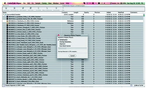
• Wait for the completion of the four fundamental steps: (1) Initialization, (2) Overlap Detection, (3) Alignment and (4) Data Model Update (). This may take 1–2 min depending upon the number of sequences and the capacity of the computer.
Figure 3. An overview of the sequence alignment as seen in the CodonCode Aligner. The floating window shows the progress of the completion of the four fundamental steps: Initialization, Overlap Detection, Alignment and Data Model Update.
• The majority of the sequences will align to the reference sequence and form a contig (Contig1). However, there may be some hundreds of sequences still remaining to be unassembled, which is primarily due to lack of significant identity to the reference sequence. This problem can be fixed either by lowering the matching threshold or by assigning another reference sequence. The latter option can be performed as described above for Contig1. !CAUTION These contigs (regardless of the number) can be combined into a single working contig (see Editing of the alignment).
(5) Editing of the alignment
Editing of the aligned sequences is important not only to ascertain the quality of the alignment but also to evaluate the alignment length vs. the sequence length of interest. In particular, beyond the length of sequence of interest (the NS1 gene in this case) needs to be trimmed. This trimming is crucial both for making the length of the entire sequences equal and for combining the different contigs into a single working contig.
• Select the “Contig1” in the user interface of the CodonCode Aligner.
• Select “Contig” in the “View” dropdown menu in the main bar.
• A new window will open which will display both the sequence name (turquoise color) and the sequence (green color). !CAUTION Note the consensus sequence at the bottom of this window labeled as “Contig1.” Selecting nucleotides in this consensus will select the corresponding nucleotides in the entire alignment.
• Locate the desired length of the gene of interest. Since the NS1 gene extends from the start codon (ATGG) to 680 nucleotides, the excess sequences beyond this length are to be trimmed. !CAUTION For easy location of the desire length, it is recommended to first remove the gaps (-) from the alignment by choosing the nucleotide in the consensus sequence and deleting by pressing back arrow.
• Mark the trimmable nucleotide(s) in the consensus, to select in the entire alignment. Alternatively, place the curser on the trimmable nucleotide in the consensus sequence and go to “Edit” in the main menu and click on “Select from start to here” to trim the sequence from the 5′ end or “Select from here to end” to trim sequence to the 3′end.
• Close the display window and return to the alignment user interface.
• Arrange the sequences according to their length in the contig by clicking on “Length.”
• Remove the sequences that are too short to be included for phylogenetic analysis by dragging the sequence(s) into the “Trash.”
• Save the alignment in Fasta format by selecting File > Export > Assembly, and label it as Contig1. You may need to choose Fasta option while exporting the assembly.
• Repeat the same editing protocol (step 5) for Contig2, Contig3 and so on, and save them with corresponding names.
• Combine all of these contigs into a single contig by adding all of them into another project in CodonCode Aligner. Assemble the contigs by clicking on “Assemble” in the CodonCode Aligner user interface.
• Export the assembled sequences in the Fasta format, and label the assembled data set as “AllNS1Genes_Assem.” !CAUTION It is possible to save this data set in the Phylp format that will be used in downstream analyses. However, by doing this it is then not possible to save the entire sequence name in the assembled sequences. By default, CodonCode Aligner, as per most other software, will save only the first ten characters, which is not sufficient for efficient tree annotation.
(6) Conversion of data sets into a readable format
It is of importance to keep the entire sequence name in the alignment and subsequent phylogenetic tree, which is required not only to trace back to the original sequence but is also the only way to annotate the tree based on host, species, subtype, continent or year. To address this problem, a Perl script can be written with special emphasis on keeping the entire sequence name while still making readable Phylp format file. There are a few fundamental requirements in this format, which include: (1) the first line must contain the number of sequences (n = 20341) and their length (l = 680) separated by at least one space, (2) the next lines contain a sequence label followed by at least one space or tab followed by the sequence characters, (3) this format allows sequence characters (for both nucleotide and amino acid) only as defined by IUPAC, (4) additionally, this format allows gaps such as (-) or (?) for nucleotide sequences and (*) (-) or (?) for protein sequences and (5) none of the characters are case-sensitive. Keeping these requirements in mind, a Perl script can convert to the desired format, as described below:
• Make a folder in your user home directory entitled “phylogenetic_tree.”
Download the Perl script (Sup. Material 2) and place it in the folder “phylogenetic_tree.” Alternatively, the Perl script was submitted to GitHub and is available to download at https://github.com/drmuhammadmunir/perl/blob/master/ConvertFastatoPhylip.
• Additionally, move the aligned data set (AllNS1Genes_Assem) file to the same folder.
• Open a “Terminal” by searching in Spotlight (right top corner in MacOSX).
• Make sure to be in the home user directory by typing “pwd.”
• Visualize the folders and directories in the home page and note the folder “phylogenetic_tree.” To do so, type “ls.”
• Move into the folder “phylogenetic_tree” by typing “cd phylogenetic_tree” and confirm the contents by typing again “ls.” !CAUTION In this folder you must have at least two files (1) ConvertFastatoPhylip.pl and (2) AllNS1Genes_Assem.fas.
• Run the following command for the format conversion: perl ConvertFastatoPhylip.pl AllNS1Genes_Assem.fas AllNS1Genes_Assem.phl
• When it is finished you will see “All done!.” !CAUTION You may observe errors such as “Illegal octal digit ‘8’ at AllNS1Genes_Assem.fas line 3431, at end of line.” In this case, open the AllNS1Genes_Assem.fas file in TextEdit and remove all of the illegal characters (see above).
• Once it is properly converted, you will see a file with the .phl extension, such as AllNS1Genes_Assem.phl in the same folder.
• Open the .phl (Phylip) file in TextEdit and compare it to the Fasta formatted file of the same data set. !CAUTION The first line of the .phl file must show “20341 680” which indicates the number of sequences and the length of the alignment, respectively.
(7) Construction of a phylogenetic tree
Several programs are available, either based on a command-line or GUI interface, to construct the phylogenetic tree. However, RAxMLGUI is used in this protocol owing to its speed and accuracy. Follow these steps to construct a fast and trustable phylogenetic tree:
• Launch the RAxMLGUI program. You will see two windows: (1) raxmlGUI 1.1, the actual user interface, and (2) raxmlGUI 1.1 console, a Python platform for background processing of the commands.
• In the raxmlGUI 1.1 window, click on the “Load alignment” button to open the alignment. !CAUTION Remember to open only the Phylip file with .phl extension.
• In the raxmlGUI 1.1 console window you may observe an error labeled as “Illegal characters in taxon-names are: tabulators, carriage returns, spaces, “”:, “,,” “),” “(,” “”;, “],” “[,” “'” Exiting.” In this case you need to open the final alignment file in TextEdit and remove these characters, as described above. !CAUTION Remember to save the changes before opening in raxmlGUI 1.1 again.
• Clear the previous alignment and re-load the alignment devoid of any illegal character.
• When the alignment uploads successfully, several messages will appear in the raxmlGUI 1.1 console window, which will be like this: IMPORTANT WARNING: Sequences CY064173_A/ring-necked_duck/Minnesota/Sg-00068/2007_H10N7_Ring-Necked_Duck and CY097594_A/mallard/Missouri/129/2009_H6N2_Mallard are exactly identical. This indicates identical sequences in the same alignment.
• You can either include or exclude these identical sequences in the construction of the phylogenetic tree. At the end of alignment upload, a pop-up window will appear in the raxmlGUI 1.1 window with the following message: RAxML found at least 1 sequence that is exactly identical to other sequences and/or gap-only characters in the alignment. Do you want to exclude it/them from the analysis? Select either “No” or “Yes” based on your preferences. !CAUTION In either case a data set will be generated and saved in the same folder where the “AllNS1Genes_Assem.phl” was uploaded with another name, “AllNS1Genes_Assem.phl.reduced.” This latter file is devoid of any repeated or identical sequences.
• Upon successful uploading of the alignment, select and modify the tree parameters in the raxmlGUI 1.1 windows. One can choose “fast tree search” for a quick and dirty tree; however, it is recommended to select the maximum likelihood (ML) + rapid bootstrap method. Accordingly, choose the number of bootstraps under the “reps.” dropdown menu ().
Figure 4. Processing of the data set for the construction of a phylogenetic tree in the raxmlGUI program. Please note two different windows, raxmlGUI 1.1 and raxmlGUI 1.1—Pythone—132 by 15. The progress of the tree construction will be displayed in the latter window.
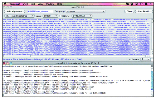
• After setting the parameters, run the program by clicking on “Run RaXML.” !CAUTION As an indication of the successful running of the program, a third window must appear called “Terminal-razmlHPC-SSE3-Ma,” which will display the progress in constructing the tree.
• At the end of tree construction, there will be five files in the same folder, which include: (1) RAxML_bestTree.AllNS1Genes_Assem.tre, (2) RAxML_bipartitions.AllNS1Genes_Assem.tre, (3) RAxML_bipartitionsBranchLabels.AllNS1Genes_Assem.tre, (4) RAxML_bootstrap.AllNS1Genes_Assem.tre and (5) RAxML_info.AllNS1Genes_Assem.tre.
(8) Annotation of the phylogenetic tree
There are different software programs available that can handle large phylogenetic trees; however, FigTree appears to be user-friendly, fast and with a few easy-click annotation possibilities. Therefore, it is used in this protocol, as described below:
• Launch FigTree and open the file named “RAxML_bootstrap.AllNS1Genes_Assem.tre.”
• In the search box (right top corner) choose “contains” and search for a sequence label that you will give a unique color in the “Color” circle. For example, a search with “H1” will highlight all sequences carrying H1 in their name. Searching with “H1N,” because all H1 will have an N in all cases, can further specify this. Doing so will minimize the chances of accidentally finding another label of H1. !CAUTION It is important to make sure that “Taxa” is selected over “Node” or “Clade.”
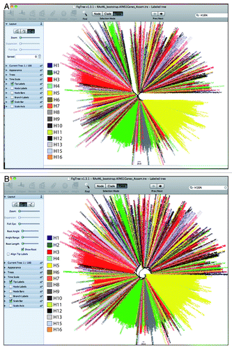
• Once annotation for the subtypes (H1–H16) of influenza viruses is completed, save the graphics in any suitable format, such as .eps or .pdf for a ready to publish figure ().
Figure 5. An overview of the tree annotated in FigTree. The clustering pattern of different subtypes of influenza viruses is highlighted with different colors. The subtypes such as H3, H5 and H6 made a bigger cluster owing to same genetic nature. All other subtypes had shown diffused pattern within the tree. For clarification purposes, only a tree of the avian influenza NS1 gene is displayed.
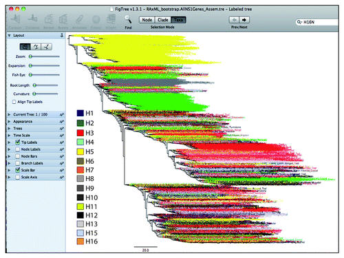
• Similarly, re-open the “RAxML_bootstrap.AllNS1Genes_Assem.tre” and label for the N gene (N1-N9) and so on for year, geographical distribution, host etc.
Conclusions
The data analyzed here provide bases for the evolution of the NS gene of avian influenza A viruses. An overall topology of the tree indicated that, based on NS gene, influenza viruses could be divided into two main groups. Although both groups contain isolates from all subtypes, the influenza viruses belonging to subtype H3, H5 and H6 constituted clear clusters within the same group of the tree. The diffused distribution of all subtypes of influenza A viruses might reflect that NS gene undergoes recombination continuously throughout the evolution history of the virus.
Timing
Throughout this process there are three steps that consume most of the time for the analysis, which include tree construction, tree annotation and sequence alignment, in descending order. However, besides these the time consumption varies, and depends upon the processing capacity of the computer and the amount of data being analyzed. The protocol presented here will require 36 h for the processing of around 20,000 sequences from preparation of data sets to annotation of the tree.
Problem Handling
The possible problems associated with this protocol are summarized in , along with their possible solution(s).
Table 1. Possible problems and their solutions
Anticipated Results
In this protocol, using the best possible combination of tools, it is anticipated to handle data sets containing thousands of sequences in comparatively little time. Moreover, this protocol is especially optimized for those scientists working with limited computer resources. The aligned sequences in Fasta format, in addition to phylogenetic tree construction, can also be used for other bioinformatics and evolutionary analyses of the pathogens. In , the final trees are displayed in different formats, each of which may suit a specific aim.
Additional material
Download Zip (1.1 MB)Acknowledgments
I would like to thank David A. Morrison for fixing linguistic errors.
References
- Shendure J, Ji H. Next-generation DNA sequencing. Nat Biotechnol 2008; 26:1135 - 45; http://dx.doi.org/10.1038/nbt1486; PMID: 18846087
- Swofford D, Olsen G, Waddel P, Hillis DM. Phylogenetic inference. Pages in (Molecular systematics, 2nd edition (D. M. Hillis, C.Moritz, and B. K. Mable, eds.). Sinauer, Sunderland, Massachusetts.
- Page R, Holmes E. Molecular evolution: A phylogenetic approach. Blackwell, Osney Mead, Oxford, UK.
- Uzzell T, Corbin KW. Fitting discrete probability distributions to evolutionary events. Science 1971; 172:1089 - 96; http://dx.doi.org/10.1126/science.172.3988.1089; PMID: 5574514
- Jin L, Nei M. Limitations of the evolutionary parsimony method of phylogenetic analysis. Mol Biol Evol 1990; 7:82 - 102; PMID: 2299983
- Yang Z. Among-site rate variation and its impact on phylogenetic analyses. Trends Ecol Evol 1996; 11:367 - 72; http://dx.doi.org/10.1016/0169-5347(96)10041-0; PMID: 21237881
- Kamel AH, Ali MA, El-Nady HG, de Rougemont A, Pothier P, Belliot G. Predominance and circulation of enteric viruses in the region of Greater Cairo, Egypt. J Clin Microbiol 2009; 47:1037 - 45; http://dx.doi.org/10.1128/JCM.01381-08; PMID: 19193841
- Stamatakis A, Ludwig T, Meier H. RAxML-III: a fast program for maximum likelihood-based inference of large phylogenetic trees. Bioinformatics 2005; 21:456 - 63; http://dx.doi.org/10.1093/bioinformatics/bti191; PMID: 15608047
- Chen F, Mackey AJ, Vermunt JK, Roos DS. Assessing performance of orthology detection strategies applied to eukaryotic genomes. PLoS One 2007; 2:e383; http://dx.doi.org/10.1371/journal.pone.0000383; PMID: 17440619
- Ebersberger I, Strauss S, von Haeseler A. HaMStR: profile hidden markov model based search for orthologs in ESTs. BMC Evol Biol 2009; 9:157; http://dx.doi.org/10.1186/1471-2148-9-157; PMID: 19586527
- Schreiber F, Pick K, Erpenbeck D, Wörheide G, Morgenstern B. OrthoSelect: a protocol for selecting orthologous groups in phylogenomics. BMC Bioinformatics 2009; 10:219; http://dx.doi.org/10.1186/1471-2105-10-219; PMID: 19607672
- Altschul SF, Madden TL, Schäffer AA, Zhang J, Zhang Z, Miller W, et al. Gapped BLAST and PSI-BLAST: a new generation of protein database search programs. Nucleic Acids Res 1997; 25:3389 - 402; http://dx.doi.org/10.1093/nar/25.17.3389; PMID: 9254694
