A point-selection algorithm based on spatial-stiffness analysis of rigid registration

Abstract

Objective: We propose a model of shape-based registration that leads to a task-specific algorithm for preoperatively selecting a set of model registration points.

Materials and Methods: We performed five sets of computer simulations using registration points generated by our algorithm and two noise amplification index (NAI) algorithms on the basis of the research of Simon . We used several different bone surface models (distal radius, proximal femur and tibia) computed from CT images of patient volunteers. The number of registration points used varied between 6 and 30.

Results: Our algorithm was faster than the NAI-based algorithms by factors of approximately 4 and 200. It had equal or better performance in terms of target registration error (TRE) when compared with the other algorithms. Our simulations also showed that point selection can have a large effect on TRE behavior; in particular, poor point selection does not necessarily decrease TRE as more registration points are added.

Conclusions: Our point-selection algorithm produces model registration points with similar or better TRE behavior than the NAI-based algorithms we tested, and it does so with significantly less computation time.

• Orthopaedic surgery
• point selection
• rigid registration
• spatial stiffness
• target registration error

Introduction

A patient's anatomy can be registered to preoperative 3D medical images for use in image-guided surgery by digitizing anatomical registration points on the patient and matching them to surface models derived from the images. We propose a method for choosing model registration points from the preoperative medical image on the basis of an extension of the method we described for fiducial registration [1]. We view the registration points as the locations where an elastic suspension system is attached to a rigid mechanism. By analyzing the stiffness matrix of the mechanism, we are able to compute a stiffness-quality measure that characterizes the least-constrained displacement of the mechanism with respect to a point target. The analysis yields the direction of translation, or the axis of rotation, of the least-constrained displacement. The form of the stiffness matrix suggests a way to add a new point to stiffen this displacement, thereby improving the quality measure.

A common problem in mechanics is determining the relationship between the displacement of a mechanism and the reaction forces that arise. This stiffness relationship is taken to be linear for small displacements about an equilibrium configuration and is characterized by a 6 × 6 spatial stiffness matrix. Consider an unloaded linear spring: the reaction force that arises when the spring is stretched or compressed along its length by a small amount x is F = kx, where k is the scalar spring constant. More generally, for an unloaded, unconstrained elastic mechanism, the force–displacement relationship iswhere the generalized force w is called a wrench and the generalized displacement t is called a twist. The symmetric 6 × 6 matrix K is called the spatial-stiffness matrix; the block matrices A, B, and D are all matrices of size 3 × 3. Properties of the spatial stiffness matrix have been discussed by many researchers [2–11].

Simon [20] proposed a method, closely related to our spatial-stiffness approach, for preoperatively choosing registration point sets. The method required calculating the eigenvalues of a 6 × 6 matrix that he called the scatter matrix; in fact, the scatter matrix is the same as the spatial-stiffness matrix that we define for shape-based registration. He referred to the problem of selecting good registration points as constraint analysis. He proposed that the noise amplification index (NAI) was one way to quantify the amount of constraint provided by a set of registration points, and his algorithm for selecting registration points attempts to maximize the value of the NAI; the NAI is defined in the Materials and methods section. Simon provided evidence that point sets with large values of NAI were associated with smaller values of his measure of registration error. The variance of registration error was also lower for point sets with large NAI. He further showed that the NAI was an approximate estimator of worst-case registration error. When compared with expert-selected point sets, the point sets synthesized using an NAI-based algorithm generally had smaller registration errors when the number of points was small; this difference tended to disappear when the number of points was greater than 25.

Materials and methods

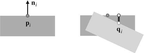
Our spatial-stiffness model of surface-based registration is illustrated in Figure 1. We parameterize the model by N surface points with locations {p_i} and unit normal vectors {n_i} for i = 1, … , N. Consider what occurs when a small displacement made up of a translation δ = [t_x t_y t_z]^T and a rotation R = R_z(ω_z) R_y(ω_y)R_x(ω_x) is applied to the registration points. The new locations of the displaced registration points are given by q_i = Rp_i + δ. For small displacements, we can assume that the region around each p_i is locally planar. The squared distance between q_i and the nearest point on the surface is given by ((q_i − p_i) · n_i)². The potential energy U_i stored in each linear spring (with the spring constant taken to be unity) connecting q_i and the nearest surface point is . It can be shown that the upper-triangular part of the symmetric Hessian matrix H_i of U_i evaluated at equilibrium iswhere p_i = [x_i y_i z_i]^T, , , , and .

Figure 1. Detail of the spatial stiffness model in the region around one of N registration points. The registration point p_i with surface normal direction n_i in its original position (gray) is displaced to new a position q_i (white) by a small rotation and translation. The spring is attached to q_i on the displaced body and to the nearest point (outlined black) on the undisplaced body.

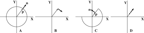
The dot products, d_xyi, d_xzi, d_yzi, have important geometric interpretations. For example, d_xyi can be computed by projecting the vectors p_i and n_i onto the xy-plane; d_xyi is the dot product of the projected p_i and a vector in the xy-plane that is perpendicular to the projected n_i. An example of the dot product d_xyi and its geometric significance is illustrated in Figure 2.

Figure 2. Two examples of the dot product d_xy. (A) A point p on a circle in the xy plane and its associated surface normal n. (B) The projection of p onto the xy plane; n is also projected but then rotated 90° in the plane. The dot product of the two vectors shown is d_xy = 0; p provides no rotational constraint about the z axis. (C) A point p on an edge in the xy plane and its associated surface normal n. (D) The projection of p onto the xy plane; n is also projected but then rotated 90° in the plane. The dot product of the two vectors shown is d_xy = ‖ p ‖; p provides good constraint about the z axis.

The spatial-stiffness matrix for surface registration is:

where

Analysis of spatial stiffness

Our method for selecting registration points is based on calculating eigenvalues and eigenvectors related to the spatial-stiffness matrix K [8]. The eigenvalues of K are not immediately useful because their magnitudes change with the coordinate frame used to define K. However, it can be shown that the eigenvalues ofare frame invariant. The eigenvalues μ₁, μ₂, μ₃ of K_V are called the principal rotational stiffnesses and the eigenvalues σ₁, σ₂, σ₃ of are called the principal translational stiffnesses. The eigenvectors can be used to calculate the principal axes of translation and rotation associated with the principal stiffnesses. The principal stiffnesses are related to the amount of energy stored in the elastic system when the mechanism is displaced from equilibrium; a large rotational/translational stiffness value indicates that it is more difficult (that is to say, more energy is required) to rotate/translate the mechanism about the associated principal axis.

The screw representation of a twist is a rotation about an axis followed by a translation parallel to the axis. The screw is usually described by the rotation axis, the net rotation magnitude M, with the independent translation specified as a pitch, h, which is the ratio of translational motion to rotational motion. For a twist [12] h = ω · ϵ/‖ ω ‖², M = ‖ ω ‖, and the axis of the screw is parallel to ω passing through the point q = ω × ϵ/‖ω‖². A pure translation (where ω = 0) has h = ∞ and M = ‖ϵ ‖, with the screw axis parallel to υ passing through the origin. A unit twist has magnitude M = 1, in which case, for ω ≠ 0, h = ω · ϵ, and q = ω × ϵ. For a small screw motion with M = α and ω ≠ 0, a point located at a distance ρ from the screw axis will be displaced by lengthBecause the principal rotational and translational stiffnesses have different units, they cannot be directly compared with one another. One solution is to use Equation 6 to scale the principal rotational stiffnesses by an appropriate factor [8] yielding the so-called equivalent stiffnesses, μ_eq,i:where, μ_i is an eigenvalue of K_V with an associated eigenvector ω_i, and ρ_i is the distance between the point of interest and the screw axis of the twist . The equivalent stiffnesses can be compared with the principal translational stiffnesses, which leads to the stiffness quality measure Q = min(μ_{eq, 1}, μ_{eq, 2}, μ_{eq, 3}, σ₁, σ₂, σ₃). Q characterizes the least constrained displacement of the mechanism. Therefore, maximizing the smallest rotational and translational stiffnesses will minimize the worst-case displacement of the mechanism. We use Q as the basis for a point-selection algorithm that builds a registration point set by sequentially choosing points that result in the largest increase in Q.

The matrix A_i in Equation 3 has only one non-zero eigenvalue σ; its associated eigenvector is . It must be the case that σ = 1 because the trace of A_i is and the sum of the eigenvalues is equal to the trace of a matrix [13]. The single non-zero eigenvalue indicates that a registration point p_i only contributes to the translational stiffness in the direction parallel to its normal vector n_i. There is a simple geometric explanation for this prediction: the region surrounding p_i is planar, so translation of p_i in this plane induces no extension of the spring attached to p_i because p_i never leaves the surface. If Q corresponds to a translational stiffness σ_min then it is easy to find the model point that produces the largest increase in Q, by selecting the model point with normal vector n most closely aligned in direction with the principal axis associated with σ_min. It turns out that the principal axis associated with σ_min is parallel to the eigenvector υ_min associated with σ_min. The point with normal vector most closely aligned in direction with υ_min maximizes the quantity (n · ϵ_min)². Alternatively, a rotation R can be applied to the surface model so that Rυ_min is parallel to the z axis; the rotated point with the largest value of should be chosen. Applying the rotation is much less efficient than simply computing a dot product, but it illustrates the approach that is required for increasing rotational stiffness.

The analysis of rotational stiffnesses is complicated by their being coupled to the translational stiffnesses. To simplify the analysis, we will ignore the coupling and focus on the matrix D that relates torque to rotational displacement. There exists a coordinate frame rotation that diagonalizes D [2] and the eigenvalues of this diagonal matrix are equal to the diagonal elements, which are the squared dot products . Suppose the rotation about the z axis needs to be stiffened. This can be done by choosing a new point p_i with normal vector n_i so that is maximized. This leads to a heuristic for stiffening the rotation about the least-constrained rotational axis: Apply a coordinate frame transformation so that the axis passes through the origin and is aligned with the z axis, then find the transformed point with normal vector that maximizes . This heuristic is not optimal, because it ignores the coupling with the translational stiffnesses. Moreover, it is not coordinate-frame invariant. However, the analytic expression to be maximized is simple to compute and is intuitively appealing.

A greedy selection algorithm

We propose an algorithm based on a simple greedy heuristic: choose the next registration point such that the increase in the value of Q is maximized.

• Choose an initial set P₀ of six registration points.

• P = P₀

• For i = 7, 8, … N

  • (i) Compute the quality measure Q.

  • (ii) If Q corresponds to a translational stiffness

    • (a) Choose p_i with n_i from the rotated model such that δ Q = (n_i · ϵ)² is maximized.

  • (iii) If Q corresponds to a rotational stiffness

    • (a) Translate and rotate the surface model so that the least-constrained rotational axis passes through the origin and is parallel to the z axis.

    • (b) Choose p_i with n_i from the translated and rotated model such that is maximized.

    • (c) Undo the transformation applied to p_i and n_i.

  • (iv) P = {P, p_i}

  • (v) Optional: Remove p_i from the set of model points.

The initial set of registration points P₀ should be chosen, so that the stiffness matrix calculated using Equation 3 is positive definite. The 3:2:1 fixturing concept [14] is a useful rule for manually choosing these 6 points.

The time complexity of this algorithm is O(MN), where M is the number of model points and N is the total number of registration points. The algorithm is not optimal, because it only tends to increase Q with each new point instead of genuinely maximizing Q. However, it is easy to implement and seems to work in practice. We will refer to this algorithm as Q_seq.

The NAI and registration

Explicitly expanding Simon's [20] expression for the scatter matrix produces a matrix that is identical to the stiffness matrix given by Equation 3. The NAI for any square matrix iswhere λ_min and λ_max are the smallest and largest eigenvalues of the matrix, respectively. The NAI was originally proposed for robot calibration purposes [15], where it was shown that maximizing the NAI led to good calibration results. Simon proposed finding the N points from M model points that maximize the NAI for registration point set selection. An exhaustive search algorithm would require examining all subsets of N registration points from the M surface model points (Simon allowed points to be chosen with repetition). Simon examined several algorithms that found local maximizers of the NAI; all of them were based on random sampling followed by optimization. He examined hillclimbing methods, a genetic algorithm, and population-based incremental learning as optimizers of NAI [16]. The major disadvantage of these methods is that they are computationally expensive. Also, they only produce point configurations that are local maximizers of NAI. In this article, we use Simon's hillclimbing algorithm to maximize the NAI, and refer to it as NAI_max. NAI_max has two adjustable parameters: the number of times the algorithm is run from a random initialization (N_trials) and the number of iterations the algorithm is allowed to run before termination (N_iter). This algorithm is not appropriate for online use because the point set of size N + 1 is constructed independently of the set of size N.

The obvious heuristic for sequentially maximizing the NAI is to choose the next point that results in the highest NAI.

• Choose an initial set P₀ of 6 registration points.

• P = P₀

• For i = 7, 8, … N

  • (a) Choose p_i with normal n_i from the surface model points so that the NAI of {P, p_i} is maximized.

  • (b) P = {P, p_i}

  • (c) Optional: Remove p_i from the set of model points.

The time complexity of this algorithm is O(MN). We have observed that this algorithm has the undesirable property of decreasing the NAI when moving from N to N + 1 points. We will refer to this algorithm as NAI_seq.

Experimental validation

The concept of target registration error (TRE) [17] is a natural measurement of registration error for our purposes because our point-selection algorithm requires that a point target be specified as input. Suppose the locations of the target in the patient coordinate frame and the coordinate frame of the computer model are x_patient and x_model, respectively. Given a registration transformation T that maps points in the patient frame to points in the model frame, the TRE is defined aswhere ‖ · ‖ denotes Euclidean distance. The TRE is simply the discrepancy in distance between the registered physical target and the target identified on the computer model of the patient's anatomy.

The selection algorithms produce model registration points defined in the coordinate frame of the computer model of the patient's anatomy. In a computer-assisted procedure, patient registration points defined in the coordinate frame of the patient are used. Our simulations generate patient registration points by adding point localization noise to the model registration points and applying a random, rigid transformation. Point-localization error (PLE) is the uncertainty in the measurement of a patient registration point. Our experiments used isotropic, normally distributed, zero mean measurement errors. Thus, the PLE is characterized by the variance of the measurement error.

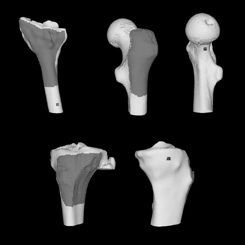
The point-selection algorithms were evaluated in terms of TRE by performing simulations of shape-based registration using points sampled from a variety of surfaces. Specifically, we used the distal end of a radius, the proximal end of a femur, and the proximal end of a tibia. The surfaces were computed from CT scans of patient volunteers using a combination of manual segmentation and the Marching Cubes algorithm [18]. Because the NAI-based algorithms are known to be sensitive to the choice of coordinate frame, all of the models were translated so that their centers of mass coincided with the origin. The surgically accessible region of bone and a point target was identified on each surface model. Images of the bone surfaces and target locations are shown in Figure 3.

Figure 3. Computer models of the bone surfaces used in the simulations. Dark gray regions are the regions from which registration points may be selected. Targets are marked by the dark gray cubes. On the distal radius model (top left), the target is the approximate location of a screw hole for a plate used to fixate an osteotomy performed to correct a fracture malunion. On the proximal femur model (top center and right), the target is the approximate location of an osteoid osteoma. On the proximal tibia model (bottom), the target is a point on the hinge of a closing wedge osteotomy.

Six sets of simulations were performed to assess the performance of Q_seq versus the NAI-based algorithms. All simulations were performed using N = 6, 7, …, 30 registration points and an isotropic point-localization noise variance of . Q_seq, NAI_max, and NAI_seq were used to generate the point sets. We chose the option of removing a point from further consideration after it had been selected when using the sequential algorithms, and we allowed repeated selection of the same point when using NAI_max. NAI_max was run using N_trials = 10 and N_iter = 10. The sequential selection algorithms (Q_seq and NAI_seq) were initialized with the same set of 6 points obtained using NAI_max with N_trials = 1000 and N_iter = 15. The generated point sets of sizes 9, 18, and 30 are shown in Figures 4–6. The input to each simulation was the surface, a set of registration points, a point target, and the (isotropic) variance of the point-localization noise magnitude. The output was the average TRE.

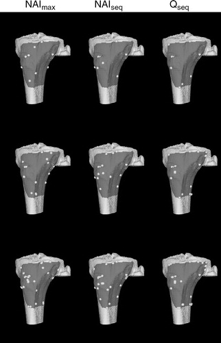
Figure 4. Distal radius surface model and registration points generated using the point-selection algorithms. From top to bottom are point sets of size 9, 18, and 30.

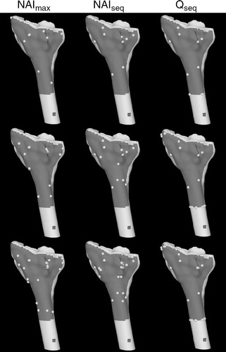
Figure 5. Proximal femur surface model and registration points generated using the point-selection algorithms. From top to bottom are point sets of size 9, 18, and 30.

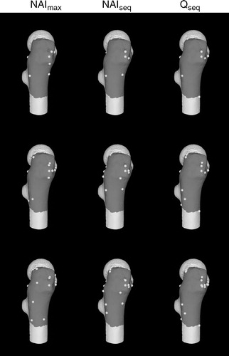
Figure 6. Proximal tibia surface model and registration points generated using the point-selection algorithms. From top to bottom are point sets of size 9, 18, and 30.

Simulation 1

In this simulation, we generated patient registration points by adding point-localization noise to the selected model registration points. Patient registration points generated in this fashion should not violate the small displacement assumption of the spatial stiffness model. This simulation was run with 10,000 trials, each trial executing the following steps:

• (1) Zero-mean, normally distributed noise was drawn from and added to the x, y, and z components of each registration-point location.

• (2) The noisy point locations were registered to the selection region using the ICP algorithm [19]. The algorithm was initialized with the true registration transformation and allowed to run to convergence in root-mean-squared error with a tolerance of 0.01 mm.

• (3) The TRE was calculated. The expected TRE was the average TRE taken over the 10,000 trials.

Simulation 2

The purpose of this simulation was to explore if the selection algorithms would cause any differences in TRE if ICP was started away from correct registration. Patient registration points were generated by adding point-localization noise and then applying a small random displacement to the selected model registration points. The displacement was specified as a rotation of 5° about a randomly generated axis passing through the origin followed by a 5-mm displacement along the axis. We did not expect that the NAI or the spatial stiffness model would be applicable after such a large displacement.

Simulation set 3

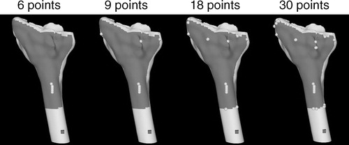
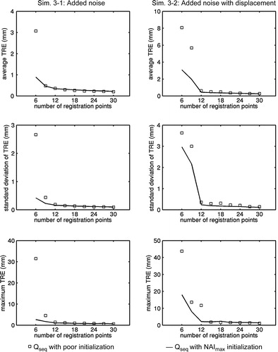
This simulation set involved only the Q_seq algorithm. It is reasonable to believe that the performance of this type of sequential selection algorithm will be dependent on the set of six points used to initialize the algorithm. Using the distal-radius model, we reran Simulations 1 and 2 with registration point sets selected by Q_seq started with an initial set of points clustered together and nearly collinear (Figure 7). This configuration of points produced an initial stiffness matrix that was poorly conditioned but still positive definite.

Figure 7. Registration points from Simulation set 3 generated on the distal radius by Q_seq starting from a set of six points that poorly constrain the registration problem. The six points are the almost collinear cluster on the shaft of the radius.

Simulation set 4

This simulation set, also involving only the Q_seq algorithm, was used to further test the validity of selecting points based on their spatial stiffness characteristics. Q_seq was modified to select the point that produced the smallest increase in the least-constrained stiffness component, that is, the modified algorithm should choose poor registration points producing higher average TREs. Using the proximal-femur model, we reran Simulations 1 and 2 with registration point sets selected by the modified version of Q_seq.

Simulation set 5

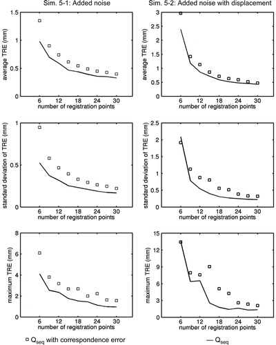
This simulation set was used to examine the effects of correspondence error, which is the error associated with localizing a patient registration point corresponding to the suggested model registration point. We used a simple model of correspondence error where it was assumed that the error had a uniform distribution over all surface points within a radius of 10 mm from the selected model point. For each trial of the simulations, each patient registration point was generated by taking the model point selected by Q_seq and sampling one point from the uniform correspondence error distribution (ensuring that the sampled point was also inside the accessible region). Simulations 1 and 2 and the proximal-femur model were used for this simulation set.

Simulation set 6

The previous simulations can be criticized because only one distinct surface model was used for each bone. Another problem is that registering the points to the selection region is unrealistic because there is a possibility that the surgeon will inadvertently collect points from outside this region. Also, because Q_seq tends to select points from the boundary of the region, it may have an unfair advantage over the NAI-based algorithms if only the selection region is considered during registration.

We addressed these issues by performing another set of simulations, this time using 10 proximal-tibial surface models from clinical volunteers. A conservatively sized point-selection region was defined on each model on the medial side of the tibia. The surface models used for registration were the entire tibias minus the areas that are normally inaccessible during medial osteotomy (the tibial plateau, posterior surface, and lateral surface). All three point-selection algorithms were used to generate registration point sets on the 10 models. Unlike the previous simulations, we chose to run Q_seq on the original bone models rather than the centered bone models used for the NAI-based algorithms. Simulations 1 and 2 were re-run with 10,000 trials and a PLE of s_PLE = 0.5 mm.

For the ith tibial model, we computed the average TRE as . We then computed the average of the 10 average TREs, , the standard deviation of , and the maximum TREs over all of the models and trials.

Results

The normalized run times for the selection algorithms, on a surface model with M = 3065 points, are shown in Table I. All timing results were obtained in Matlab (The MathWorks, Inc., Natick, MA, USA) running on a SunBlade 1000 workstation (Sun Microsystems, Inc., Santa Clara, CA, USA). Q_seq was faster than NAI_seq by approximately a factor of four. This was not surprising, because NAI_seq must solve an eigenvalue problem for every model point. Q_seq was faster than NAI_max by approximately two orders of magnitude. NAI_max requires more execution time than Q_seq because it attempts to find a globally optimal set of registration points.

Table I.  Normalized run times of the point-selection algorithms for M = 3065. Actual run times have been divided by the amount of time required by Q_seq to generate a point set of size 9.

Algorithm	Number of registration points
	9	12	15	18	21	24	27	30
Qseq	1	2	3	4	5	6	7	8
Nseq	4	8	12	16	21	25	29	33
NAImax	180	450	800	1100	1500	2000	2600	3300

Simulations 1 and 2

Graphs of TRE versus number of registration points are shown in Figures 8–10 for the three bone surfaces. In the distal radius simulation with only point-localization noise, Q_seq outperformed the NAI-based algorithms. With the application of an initial displacement, Q_seq had remarkably good and stable performance after only 12 registration points. NAI_max required 21 points to match Q_seq in terms of average TRE, and NAI_seq never matched the performance of the other algorithms. Q_seq had the best worst-case TRE performance. Given the clear differences in the pattern of point distribution between the NAI and stiffness-based algorithms, it is not surprising that there were consistent differences in the TRE results.

Figure 8. Results for Simulations 1 and 2 using the distal radius model. From top to bottom are average TRE, standard deviation of TRE, and maximum TRE.

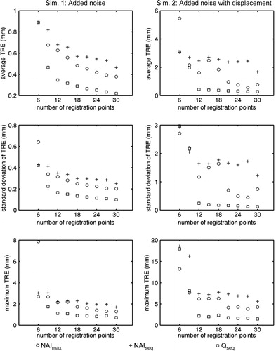
Figure 9. Results for Simulations 1 and 2 using the proximal femur model. From top to bottom are average TRE, standard deviation of TRE, and maximum TRE.

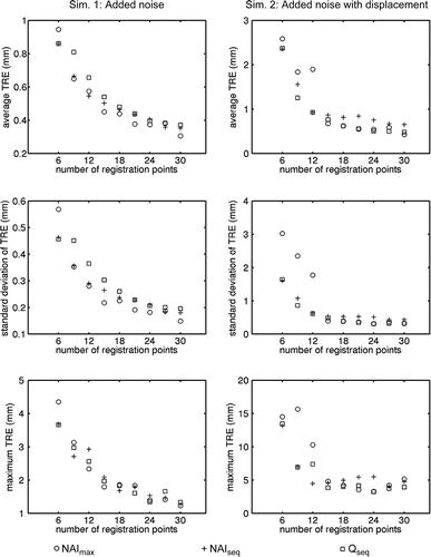
Figure 10. Results for Simulations 1 and 2 using the proximal tibia model. From top to bottom are average TRE, standard deviation of TRE, and maximum TRE.

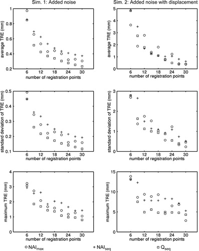
The point distributions for the proximal femur model were visually the most similar, and the TRE results were similar as well. There were no clear differences in TRE for point sets larger than 15 in either simulation.

In the proximal tibia simulation with only point-localization noise, Q_seq outperformed the NAI-based algorithms. In the second simulation, Q_seq usually produced the smallest worst-case TRE. The erratic performance of NAI_max was probably caused by NAI_max constructing point sets independently of one another rather than building sequentially on smaller point sets.

It is interesting that, for all three models, the average TRE and the worst-case TRE tend not to decrease after 15 points for the best performing algorithms in the simulations with an initial displacement.

Simulation set 3

The results for this simulation set are plotted in Figure 11. When there was only point-localization noise, the TRE behavior of the point set initialized with clustered, nearly collinear points was effectively the same as the point set used in Simulations 1 and 2 after a total of 9–12 registration points. With the addition of an initial displacement, the behavior in TRE was almost identical for both point sets after 12–15 points.

Figure 11. Results for Simulation set 3 using the distal radius model with points generated using Q_seq initialized with a set of six points that poorly constrain the registration problem. From top to bottom are average TRE, standard deviation of TRE, and maximum TRE. The solid lines are the results obtained using a good initial set of points. The results are identical to those shown in Figure 7.

Simulation set 4

The results for this simulation set are plotted in Figure 12. The version of Q_seq modified to select poor registration points performed much worse than the original version of Q_seq.

Figure 12. Results for Simulation set 4 using the proximal femur model with a version of Q_seq modified to pick the next point that contributes the least to the worst-case stiffness component. From top to bottom are average TRE, standard deviation of TRE, and maximum TRE.

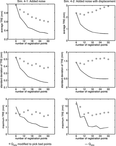
In the simulation with an initial displacement, the modified Q_seq exhibited increasing average TRE. This result was surprising as well: it suggested that it was possible to obtain increasingly worse average TRE when using more registration points. TRE variance and worst-case TRE were also higher when using point sets produced by the modified version of Q_seq.

Simulation set 5

The results for this simulation are plotted in Figure 13. Correspondence error of up to 10 mm produced higher TREs and higher standard deviation of TRE. Increasing the number of registration points reduced the magnitude of this effect.

Figure 13. Results for Simulation set 5 using the proximal femur model with Q_seq and correspondence errors. From top to bottom are average TRE, standard deviation of TRE, and maximum TRE.

Simulation set 6

The results for this simulation are plotted in Figure 14. In the simulations with only added noise, Q_seq had better performance than the NAI-based algorithms, but the differences were small. Q_seq also slightly outperformed the NAI-based algorithms in the simulations with an initial displacement. Again the actual differences in performance were small.

Figure 14. Results for Simulation set 6 using 10 different proximal tibial models. The top row shows the average of the 10 average TREs (), the second row shows the standard deviation of , and the third row shows the maximum TRE over all 10 models.

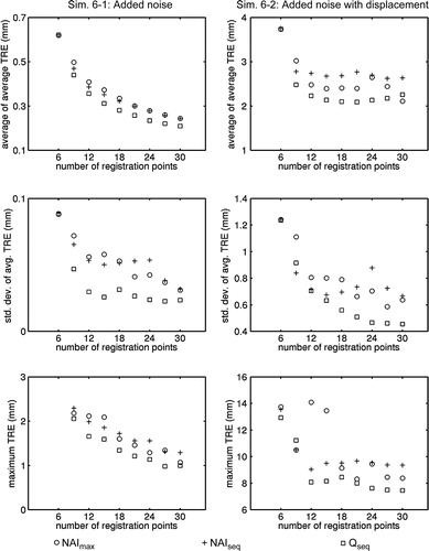
When we looked at the results for each bone, we found that Q_seq produced the lowest maximum TRE in 8 of the 10 cases. It produced the lowest average TRE in 5 of the 10 cases. We believe that the performance of our algorithm would have been better if we had used the same centered computer models used for the NAI-based algorithms.

Discussion

One weakness with our experiments was that the TREs obtained using NAI_max are possibly overestimated because of the difficulty in finding the global maximum of NAI. Q_seq is not a global optimizer of its stiffness criteria, but its performance was on par with, if not better than, NAI_max, and required substantially less computation. The sequential NAI algorithm, NAI_seq, generally had the worst performance of the three algorithms. Finding an optimal solution to batch point selection, which would automate the preoperative selection of registration points, remains an open problem.

Another weakness of our experiments was that the simulations were intended to examine how point selection affects TRE, but the TRE values are inextricably linked to the registration algorithm. This almost certainly had some effect on TRE in the simulations with the displaced point sets, but we would be surprised if there was a strong effect on TRE for the simulations with only added noise. Furthermore, the simulations with the modified version of Q_seq clearly demonstrated that point selection can have a profound effect on TRE behavior. An unknown issue is to what degree point selection affects registration accuracy in clinical practice.

The option of removing a model point after it has been selected does not have any significant effect on the behavior of TRE if the surface models are densely sampled because points adjacent to the removed point will have similar location and normal vectors. If the surface models are coarsely sampled, then there may be a noticeable effect on TRE, but we have not explored this issue.

Our model of correspondence error was similar to the data collection uncertainty model used by Simon [20]. Our model assumed identical, independent, spatially uniform distributions of error surrounding each suggested model point. This assumption is overly simplistic because distinct anatomical points should have smaller correspondence errors than less easily identified anatomical points. We also expect some correlation in the correspondence errors for closely spaced registration points.

Simon [20] observed that the NAI was more sensitive to variations in normal direction than point location. This is not surprising, given the form of the stiffness matrix: the components of the normal vector appear everywhere, whereas the components of point location appear only in the submatrices B and D. In terms of the spatial-stiffness analysis, the normal vectors affect both the translational and rotational stiffnesses, whereas the point locations only affect the rotational stiffnesses. One implication of normal-vector sensitivity is that the point-selection algorithms are unreliable when the surface models are noisy. A denoising algorithm [21] can effectively compensate for small-scale noise, but we suspect that the point-selection algorithms will perform poorly in high-noise conditions. This also suggests that denoising algorithms that preferentially reduce the local variability of surface normals would be particularly useful.

Simon [20] needed to uniformly scale his models so that he could compare the six eigenvalues of his scatter matrix. The approach we have presented scales the eigenvalues instead of the model: the principal rotational stiffnesses are scaled based on the location of the target relative to the principal axes, which eliminates the need to scale the model. A minor advantage of Simon's approach is that it does not require a target location. However, the stiffness-based approach produces a task-specific choice of registration points based on a point target, which is advantageous when a surgeon seeks to optimize the registration around a particular anatomical site.

Q_seq is based on the assumption that the TRE is dominated by one poorly constrained stiffness component. In theory, Q_seq should be suboptimal in terms of reducing the expected TRE, because the maximum increase in worst-case translational/rotational stiffness leads to a minimal increase in the remaining four translational/rotational stiffness components. Furthermore, the results of Simulation set 6 suggest that Q_seq is sensitive to the choice of coordinate frame (although the spatial-stiffness analysis is not); exactly what significance the choice of coordinate frame has needs to be clarified. We are investigating alternative point-selection algorithms that do not have these deficiencies.

An attractive feature of Q_seq is that it selects the next best registration point given the current set of registration points. This feature would be especially useful intraoperatively by providing the online capability of dynamically guiding the surgeon to good registration points. Unfortunately, the stiffness model requires that the model registration-point locations and orientations be known. That is to say, the registration needs to be known in order to establish a good estimate of the correspondence between the digitized patient points and the model surface points. If the registration is known, there is no need to acquire additional registration points, and if the registration is unknown, the stiffness matrix cannot be computed. Of course, an estimate of the registration or the correspondences could be used, but this would not account for the uncertainty in the estimate. We are investigating the feasibility of combining Q_seq with a registration algorithm that generates estimates of the registration uncertainty to provide online guidance of registration-point selection.

Acknowledegments

This research was partly supported by the Institute for Robotics and Intelligent Systems, the Ontario Research and Development Challenge Fund, and the Natural Sciences and Engineering Research Council of Canada.

References

- Ma B, Ellis R E (2003) A spatial-stiffness analysis of fiducial registration accuracy. Proceedings of the Sixth International Conference on Medical Image Computing and Computer-Assisted Intervention (MICCAI 2003), MontréalCanada, November, 2003, R E Ellis, T M Peters. Springer, Berlin, I: 359–366
- Lončarić J. Normal forms of stiffness and compliance matrices. IEEE J Robot Automat 1987; RA-3(6)567–572
- Lipken H, Patterson T (1992) Geometrical properties of modelled robot elasticity: Part II – center of elasticity. Proceedings of the ASME Design Technology Conferences, Scottsdale, AZ, September, 1992. ASME, New York, DE-Vol. 45: 187–193
- Patterson T, Lipkin H. Structure of robot compliance. ASME J Mech Des 1993; 115(3)576–580
- Patterson T, Lipkin H. A classification of robot compliance. ASME J Mech Des 1993; 115(3)581–584
- Ciblak N, Lipken H (1994) Centers of stiffness, compliance, and elasticity in the modelling of robotic systems. Proceedings of the ASME Design Technology Conferences, Minneapolis, MN, September, 1994. ASME, New York, DE-Vol. 72: 185–195
- Bruyninckx H, Demey S, Kumar V (1998) Generalized stability of compliant grasps. Proceedings of the IEEE International Conference on Robotics and Automation, Leuven, Belgium, May, 1998. IEEE, 2396–2402
- Lin Q, Burdick J, Rimon E. A stiffness-based quality measure for compliant grasps and fixtures. IEEE Trans Robot Automat 2000; 16(6)675–688
- Roberts R G. A note on the normal form of a spatial stiffness matrix. IEEE Trans Robot Automat 2001; 17(6)968–972
- Selig J M, Ding X. Structure of the spatial stiffness matrix. Int J Robot Automat 2002; 17(1)1–15
- Žefran M, Kumar V. A geometric approach to the study of the Cartesian stiffness matrix. ASME J Mech Des 2002; 124(1)30–38
- Murray R M, Li Z, Sastry S S. A mathematical introduction to robotic manipulation. CRC Press, Boca Raton, FL 1994
- Horn R A, Johnson C R. Matrix analysis. Cambridge University Press, CambridgeUK 1985
- Shirinzadeh B. Issues in the design of the reconfigurable fixture modules for robotic assembly. J Man Sys 1993; 12(1)1–14
- Nahvi A, Hollerbach J M (1996) The noise amplification index for optimal pose selection in robot calibration. Proceedings of the IEEE International Conference on Robotics and Automation, Minneapolis, MN, April, 1996. IEEE, Piscataway, NJ, 647–654
- Baluja S, Simon D. Evolution-based methods for selecting point data for object localization: Applications to computer-assisted surgery. Appl Intell 1998; 9: 7–19
- Maurer C R, Fitzpatrick J M, Wang M Y, Galloway R L, Maciunas R J, Allen G S. Registration of head volume images using implantable fiducial markers. IEEE Trans Med Imaging 1997; 16(4)447–462
- Lorensen W E, Cline H E. Marching cubes: A high resolution 3d surface construct ion algorithm. Comput Graph 1987; 21(4)163–169
- Besl P, McKay N. A method for registration of 3-D shapes. IEEE Trans Pattern Anal 1992; 14(2)239–256
- Simon D A. Fast and accurate shape-based registration. Carnegie Mellon University, Pittsburgh, Pennsylvania December, 1996, PhD thesis
- Jones T R, Durand F, Desbrun M (2003) Non-iterative, feature-preserving mesh smoothing. Proceedings of the 30th International Conference on Computer Graphics and Interactive Techniques (SIGGRAPH 2003), San Diego, CAUSA, July, 2003. ACM Press, New York, 943–949