Abstract
This article discusses an active learning technique that can be easily incorporated into a variety of introductory statistics classes to demonstrate purely subjective and statistical confidence intervals. The concepts of confidence intervals, confidence levels, and the fixed, but unknown, population parameter are frequently misunderstood by a significant proportion of students. This class activity demonstrates these concepts by stressing the objective nature of statistical confidence intervals. It also emphasizes that the precision of the interval depends on the quality of the data used in its construction. The proposed exercise takes less than 50 minutes of lecture time and helps to solidify these essential statistical concepts in a visual and memorable way. Student reaction to the exercise has been positive as measured anecdotally by both improved student understanding of the concepts and increased interest in the activity.
1. Introduction
1 This exercise is currently used in introductory statistics courses for non-statistics majors in a variety of different disciplines, including engineering, mathematics, and the biological, physical, and social sciences. The goal of the exercise is to present visually the concept of the confidence level and the fixed, but unknown, nature of the parameter being estimated. The activity emphasizes the objective nature of the confidence interval and how the precision of the interval depends on the quality of information obtained through appropriate sampling strategies.
2 A key feature of the exercise is that the students are actively engaged in the demonstration of the concepts, which is essential for increasing student learning (Angelo 1993). This interaction with students and their involvement in all phases of the activity help to solidify difficult statistical concepts.
3 The activity consists of three phases. In Phase 1, the students naively give a purely subjective “95% confidence interval” for a fact about which they have some intuition, but likely no precise knowledge. A plot of their intervals is shown, and some discussion follows about what the “95%” measures. In Phase 2, students employ the same purely subjective interval construction method for a different fact, but now they should have a better understanding of the conditions the intervals are expected to satisfy.
In both phases, students tend to make their intervals too narrow, and hence, the intervals do not include the true parameter with appropriate frequency. Phase 3 makes the transition from a purely subjective interval to a statistical confidence interval. In Phase 3, students examine the similarities and differences between the two types of intervals. Phase 3 concludes with a demonstration of constructing confidence intervals for the mean of a normal population using simple random samples. This phase can also include a discussion of distributional assumptions and sample size requirements for the use of statistical confidence intervals.
4 The exercise requires less than a single lecture (I typically take approximately 40 minutes to run through all of the demonstrations and discussion), and requires active participation from the students. The ideal class size for the activity is around 40, but it will work for classes of size 20 to 100. If the class is too small, it may be difficult to illustrate the 95% confidence level effectively. If the class is much larger than 40, only a subset of students should be used at each of Phases 1 and 2.
5 Materials required include a fact sheet (), two or three file cards or small pre-cut pieces of paper for each student in the class, and an overhead projector with several gridded transparencies (a transparency made from a photocopied piece of graph paper works well). Alternately, the transparencies can be replaced with a projection screen and laptop computer, if the S-Plus functions in Appendix 1 are incorporated into the demonstration. This second approach allows for slightly faster presentation of the data, but both methods work well.
Table 1. Confidence Interval Estimation Facts (Based on 1996 Data)
2. Details of the Activity
6 Typically, this activity is run early in the unit on estimation, but after students have had some introduction to probability and the normal distribution. It is helpful if there has been some discussion about how poll results are usually reported with a margin of error and a confidence level (e.g., 12% ± 2%, correct 19 times out of 20).
2.1 Phase 1
7 In Phase 1, students are asked to provide purely subjective 95% confidence intervals for a given fact (selected from the fact sheet shown in ). In addition to the facts given in , some local or state facts may also be of interest. These are readily available from almanacs or the Internet. Generally, few instructions are given to clarify what is meant by a 95% confidence interval; instead, the students are left to make their own judgments. It is helpful to give the students some scale for their estimates (e.g., “In thousands, give a 95% confidence interval for…).
8 The intervals are recorded on the file cards, collected, and summarized by a student assistant (usually a volunteer from the class). While the helper is entering the data onto the gridded overhead, it is possible to discuss what the students were thinking about when they determined the width of their intervals (i.e., their notions of “95% confident”). It is also helpful to discuss what would constitute the ideal interval (namely one that is narrow, but also correct). If transparencies are used, it is helpful to determine an upper and lower bound that includes the intervals of all of the students in the class before the cards are collected. Once all of the intervals are recorded on the overhead, a vertical line is added to show the true value of the fact under consideration. Alternately this can be done using the function “conf.int” given in Appendix 1. shows an example of what the result might look like for 20 students after completion of Phase 1.
9 Typically, far more than the expected 5% of students’ intervals will fail to include the true value in their range. In the example given, only 11 of 20 students gave intervals that included the true parameter value. This can lead to discussion about what this would mean in practice, if we quoted a 95% C.I., but the actual true confidence level was much lower.
Figure 1. Student Intervals for Phase
2.2 Phase 2
10 In Phase 2, repeat the activity in Phase 1 with a slight modification. Ask each student to give a 95% confidence interval and to provide a single best guess for a new fact. Record the intervals and point estimates. The goal of this phase is to help students formalize some of the concepts in “common sense” terms, before changing to the statistical realm, where many students seem less willing to trust their intuition.
11 Discussion of the Phase 2 intervals provides an opportunity to highlight specific results of the constructed intervals and general properties of confidence intervals. After calculating the proportion of intervals containing the true value, students can assess the accuracy of the group of confidence intervals. Quite often the majority of students will still make their intervals too narrow to cover the true value, so you may not be close to the desired 95% confidence level. Students can also be encouraged to consider how the results and desirability of the intervals would change if the desired confidence level changed to 90% or 99%. For example, the 90% confidence level allows for a narrower interval, since there is less of a burden to be correct than for the 95% or 99% confidence intervals. Examination of the point estimates can motivate discussion of the advantages of having a quantifiable success rate for the intervals, versus the simplicity of a single value for the point estimate. Finally, the merits of having the point estimate centered in the interval can be discussed.
2.3 Phase 3
12 Phase 3 involves making the transition from purely subjective intervals to statistical confidence intervals. First, some remarks should be made about common features of all interval estimates. The motivation for creating an interval is to provide a reasonable range of values that has a high likelihood of including the true parameter of interest. The ideal interval will be narrow and accurate (contain the true value). It should be clear to the students that increasing the amount of knowledge used to construct the interval should lead to a narrower, more precise interval. Again, it is helpful to highlight the lack of quantification about whether point estimates are “close” to the true value, and how confidence intervals overcome this weakness. It should be emphasized that the confidence level is based on repeated sampling (such as the construction of many intervals by members of the class), but for a given case, we usually have only a single interval under consideration. The single confidence interval is either correct or incorrect (all or nothing), but the confidence level gives us an indication of the proportion of correct intervals that can be expected with repeating the estimation procedure. Finally, once an interval is constructed, we usually do not find out if it is actually correct. This final point is worth stressing, since it helps the students focus on the difference between the sample, where all the data are available, and the population, where the true answer is typically unknown.
13 Next, some time is spent formalizing the connection between purely subjective intervals and statistical confidence intervals and highlighting key differences between the two methods. A sample from the population is similar to partial knowledge used to estimate the quantity of interest. In both the purely subjective and the statistical cases, we have some information that helps us give a range of sensible values, but the lack of complete knowledge leads to some uncertainty in the estimates. We hope that our knowledge will allow us to make a sensible estimate, but we are unsure of its accuracy. The amount of knowledge used to estimate the purely subjective interval is roughly analogous to the amount of data collected for a statistical confidence interval. As more data or information becomes available, the interval will become narrower. For a purely subjective interval, information is measured by the level of knowledge about the subject matter. For a statistical confidence interval, the width depends on the number of observations in the sample from the population of interest.
14 The quality of information used to construct the intervals and the accuracy of the intervals can also be compared. If someone with no accurate knowledge of the subject matter suggests a purely subjective confidence interval, we would not expect his or her interval to be helpful for estimating the true quantity of interest. Similarly, if a sample is not representative of the underlying population it is thought to describe, we should not expect the interval to provide an accurate estimate of the population
value.
15 The estimation of intervals by multiple students is roughly analogous to collecting multiple samples. Each student or sample produces an interval, but typically in practice, only a single interval is formed, and we do not know if the interval is correct. A key difference between methods is that given the same amount of knowledge (e.g., two students who took the same course in geography), two purely subjective intervals are unlikely to be the same, but given the same data, a single statistical confidence interval is obtained. This lack of subjectivity for the statistical method is a significant advantage.
16 Another difference between the methods is that unless we are able to determine the true value of the parameter of interest, we cannot quantify the confidence level of a purely subjective interval. However, for a statistical confidence interval, there is underlying theory that (under certain distributional assumptions) gives us an accurate confidence level for our intervals.
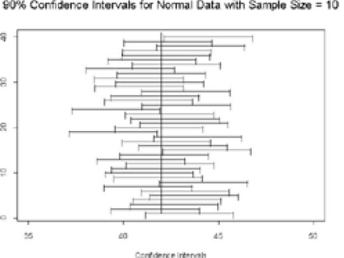
17 To conclude this phase of the exercise, two options are available. Print the figures in Appendix 2 onto transparencies or use the S-Plus functions in Appendix 1 to display results for statistical confidence intervals. The S-Plus function called “norm.conf” generates a large number of samples from a given normal distribution, and calculates the confidence interval for the mean for each sample. An example of the output from the function is given in for 40 samples of size 10 drawn from a normal distribution with mean 42 and standard deviation 4 units. Alternately, you can use , along with and in Appendix 2, to show a variety of results. These plots each show 40 intervals generated using different sample sizes and confidence levels.
Figure 2. Computer-Generated 95% Confidence Intervals for the Mean of a Normal Distribution, n = 10.
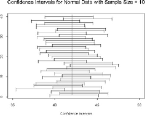
18 These figures can be used to discuss several key features of statistical confidence intervals. We can assess the true confidence level of the confidence intervals by looking at the proportion of intervals that contain the true population parameter. In the example given in , 39 of the 40 confidence intervals contain the true parameter value. This is consistent with data from a binomial distribution with probability of success equal to 0.95. Differences in observed interval widths for a fixed sample size are a reflection of the quality of the data that we observe in each sample. Increasing the sample size results in narrower confidence intervals, as can be seen in and . Decreasing the confidence level reduces the width of the confidence intervals, as shown by and . Finally, a discussion can be included of how violations of distributional assumptions can lead to incorrect confidence levels. At the end of this exercise, students have the conceptual background and the motivation to learn details about the construction of statistical confidence intervals for the mean of a normal distribution.
3. Conclusions
19 This simple exercise has been implemented successfully into several introductory statistics courses. Students appreciate the visual demonstration of concepts that have frequently been a source of confusion, and they are better able to discuss the meaning of statistical confidence intervals, confidence levels, and the advantages of interval estimation over point estimation. Feedback from the students about the activity has been positive. At the conclusion of the course, many still remember the exercise and comment on it positively. On term tests and the final exam, questions about confidence intervals seem to be answered correctly more consistently than in the past, and students are better able to verbalize these concepts. Relatively few specialized resources and only a small amount of time are required to effectively introduce this important concept and build increased statistical literacy.
Acknowledgments
Research for this paper was funded by the Virginia Tech Center for Excellence in Undergraduate Teaching. I would also like to express my thanks to Tom Wonnacott, Department of Statistical and Actuarial Sciences, University of Western Ontario, for the initial idea of constructing purely subjective confidence intervals to demonstrate this concept. In addition, I would like to thank the reviewers and associate editor for their comments, which helped to substantially improve the readability and content of the paper.
Reference
- Angelo, T. A. (1993), “A Teacher’s Dozen: Fourteen General Research-Based Principles for Improving Higher Learning in Our Classrooms,” American Association of Higher Education Bulletin, 45, 3–13.
Appendix 1:
S-Plus Functions
A.1 Function to Plot Student-Generated Subjective Intervals for a Fact With True Value “actual.val”
<fig>
A.2 Function to Generate Confidence Intervals for Samples From a Normal Distribution With Sample Size “num,” mean “mu,” and standard deviation “stdev”
<fig>
Appendix 2:
Additional Plots
Figure 3. Computer-Generated 95% Confidence Intervals for the Mean of a Normal Distribution, n = 20.
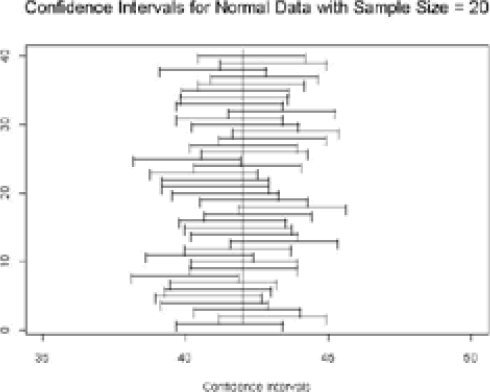
Figure 4. Computer-Generated 90% Confidence Intervals for the Mean of a Normal Distribution, n = 10.