Estimation of Heat and Mass Transfer Coefficients During Air-Freezing of Cucumber

Abstract

Freezing of foods involves coupled heat and mass transfer. It is essential to optimally design the freezing equipment and maximise the efficiency of the freezing process. Therefore, it is necessary to estimate the heat and mass transfer coefficients. In this study, the surface heat and mass transfer coefficients were estimated employing the Hilbert equation as well as the corresponding thermal and diffusive boundary layers during freezing of unpeeled cucumber at low air temperatures (−10 to −18 and −25°C). The estimated mean heat transfer coefficients ranged from 10.99 W m⁻² K⁻¹ for 0.5 m s⁻¹ up to 40.07 W m⁻² K⁻¹ for 5.0 m s⁻¹. The respective mass transfer coefficients ranged from 8.98 up to 32.40 m s⁻¹. The estimated heat transfer coefficients were compared with the respective ones calculated from Dincer and Dincer and Cengeli during air-cooling (22 to 2°C) of unpeeled cucumbers of similar size as well as other agricultural cylindrical products.

Keywords:

• Air-freezing
• Cucumber
• Heat transfer coefficient
• Mass loss
• Mass transfer coefficient

INTRODUCTION

Quality preservation is the main aim in food refrigeration. Freezing slows down chemical, biochemical reactions, and microbial activity, retarding food deterioration due to immobilisation of the available water and, therefore, reducing water activity. Freezing helps the final frozen product to sustain its initial quality during cold storage.[1] The surface heat and mass transfer coefficients are local phenomena dependent primarily from the temperature and velocity of the surrounding fluid, product geometry, orientation, surface roughness, packaging, and water vapour deficit. Studies have shown that the most significant factors affecting surface heat and mass transfer coefficients are the temperature difference and the velocity of the fluid flowing around the product. Driven from the previous findings, it is common to present the experimentally determined surface heat-mass transfer coefficients in terms of Nu-Re, Sh-Re dimensionless numbers since Pr and Sc vary insignificantly for the commercial freezing conditions. These correlations provide a good approximation of the heat-mass transfer coefficients as functions of product shape and size as well fluid velocity and temperature. A number of studies have been conducted to estimate the surface heat-mass transfer coefficients during freezing (low air temperatures) of food items.2–8 Very informative are review papers9–14 covering many conducted studies on heat and mass transfer during the freezing process; unfortunately, most of them concern meat products. Although a lot of research has been carried out on the freezing of meat products, there is also a great demand for information on frozen vegetables. One objective of this study was to investigate the response of unpeeled cucumber subjected to air-blast freezing conditions and to determine the heat and mass transfer coefficients and other related transport parameters.

MATERIAL AND METHODS

Experimental Facility

The experimental duct was designed and manufactured at the ‘Farm Machinery’ laboratory of Agricultural University of Athens, Greece. The experimental duct was operated in a well-insulated refrigerated room in which the cold air was delivered by a common commercial refrigeration installation operating with R-22. The dimensions of the refrigerated room were big enough to accommodate the experimental facility. The refrigeration installation could lower room temperature down to −30°C. The open-ended experimental duct in which the cold air was circulated was 5 m in length and rectangular. The testing chamber (30 × 80 cm) was fit into the middle of the five-part duct (Fig. 1). The air in the duct was driven by an axial fan fitted at its exit, and fan revolutions could be controlled electronically. The air velocity field was homogenised by a series of vanes fitted at the ends of the duct (Fig. 1). A convergent duct bearing a honeycomb grid at its end was fitted upstream of the test chamber. The air velocity was also regulated by a damper placed at the discharge of the fan. The air velocity was measured with a hotwire anemometer which could operate at subzero temperatures. The previous experimental arrangement could establish quasi uniform velocity profiles.

Figure 1 Experimental duct [a]: (1) sample, (2) electronic scale, (3) airflow homogenization grid, (4) vanes, (5) fan, (6) dumper. Test chamber [b]: (1) homogenization grid, (2) electronic scale, (3) sample, (4) insulation, (5) cylinders holding the sample, (6) anemometer.

The freezing-air temperature was controlled by a thermostat. A six-channel data logger (CR10X, Campbell Scientific Ltd., Logan, Utah, USA) interfaced with a personal computer was used to monitor temperature of the air in the cold store as well the temperature of the sample surface and its geometric centre. The humidity of the room was measured with an electronic thermo-hygrometer. Air samples were withdrawn using a small capacity centrifugal air pump and were driven through a 3-m tube to the previous referred thermo-hygrometer. The tube was covered by an electric resistance to warm the displaced air prior to its entrance to the hygrometer. Based on this experimental arrangement the air sample temperature was 15–20°C. The freezing samples were weighted by an electronic scale whose mechanical part was placed in the experimental duct and its electronic out of the duct to prevent malfunctions caused from the subzero temperatures.

Experimental Procedure

In the conducted experiments, two unpeeled cucumbers of cylindrical shape were used. The dimensions of the samples were 13.43 ± 1.92 cm in height, 40.87 ± 1.14 mm in diameter, 172.58 ± 25.63 cm² in surface area, and 182.44 ± 27.50 g in weight. The detailed dimensions of the tested samples in the 15 experimental cases are presented in Table 1. To ensure that heat and mass transfer were radial driven, two rubber discs were fitted at both ends of the samples. Temperature and mass loss of the samples were regularly measured during the freezing period in 2–3-min intervals. The first sample was used for weighing, while the second was used for temperature measurement. In the sample used for temperature measurement, three thermocouples were fitted hypodermically. The three thermocouples were symmetrically located around the cylindrical sample. The previous setup was chosen to ensure that weighing was not affected by the thermocouples weight. Weighing was carried out with an electronic scale having an accuracy of ±0.02 g, resolution of 0.01 g, and maximum capacity of 400 g. Thermocouples K-type of ±1.0 K accuracy and 0.1 K resolution were used.

Table 1 Characteristics of the tested cucumber samples used in the fifteen examined experimental cases

T (°C)	V(m^.s^−1)	L(cm)	D(mm)	S(cm^2)	G o (g)
−10	0.5	10.0	39.5	124.09	128.50
	1.0	14.0	40.5	178.13	190.07
	1.5	15.0	39.0	183.78	183.78
	2.0	15.0	42.0	197.92	207.73
	5.0	10.0	39.5	124.09	128.50
−18	0.5	15.0	42.0	197.92	217.88
	1.0	15.0	41.5	195.56	211.04
	1.5	13.5	41.0	173.89	182.75
	2.0	12.0	43.0	162.11	180.95
	5.0	14.0	40.0	175.93	174.80
−25	0.5	15.0	40.5	190.85	194.52
	1.0	12.0	41.0	154.57	166.23
	1.5	15.0	42.0	197.92	214.71
	2.0	11.0	41.5	143.41	162.74
	5.0	15.0	40.0	188.50	192.40

Both samples were suspended in the experimental duct 20 cm from the side wall and 7 cm from the top wall of the duct. The air temperature and relative humidity were measured with a hygrothermal sensor (Therm 2280-1; Ahlborn Mess, Holzkirchen, Germany) having for RH measurements an accuracy of ±2.0%, resolution of 0.5%, and temperature accuracy of ±1.0 K in the range 0 to 60°C. The hot wire anemometer had an accuracy of ±0.044 m s⁻¹ and a resolution of 0.1 m s⁻¹. In all cases, the measured RH was 0.65.

The freezing process was terminated when the temperature of the sample's surface reached the freezing-air temperature. The latter was controlled by an electronic thermostat that exhibited a tolerance of ±2.0 K. The tested air temperatures were −10, −18, and −25°C and the respective air velocities were 0.5, 1.0, 1.5, 2.0, and 5.0 m s⁻¹.

Analysis of the Experimental Data

Analysis of variance (ANOVA) was conducted by Statgraphics Plus.[15] The estimated mean heat and mass transfer coefficients were compared with those reported from Dincer[2] and Dincer and Genceli[16] using Tukey HSD (honesty significant difference) multiple range statistical test (P ≤ 0.05). The Tukey HSD test is based on the studentized range distribution similar to the distribution of t parameter from the t-test. The choice was based on the smaller derived Type-I error of the specific test compared to other well-known Fisher, Newman-Keuls, and Duncan multiple range tests.[17]

Thermodynamic Properties of Water at Saturation

The water vapour deficit of the freezing air ΔP _v , is defined as the difference between the water vapour pressure P _s at saturation and the partial water vapour pressure P _v exerted by the water vapour molecules in the moist freezing air at a specific temperature, as shown in Eq. (1). The water vapour pressure at saturation for the temperature range −100 up to 200°C was calculated from relations presented by Wexler and Hyland.[18]

(1)

RESULTS AND DISCUSSION

Surface Temperature and Parameters of Influence

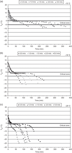
Figures 2a–2c present the surface temperature of the samples for the three air temperatures used in this study. The sigmoid shape of the surface temperature curves is characteristic of the biological materials undergoing freezing.[19] The shortest freezing time (75 min) was noted at −25°C and 5 m s⁻¹, while the longest (375 min) was noted at −10°C and 0.5 m s⁻¹. The fastest freezing case (−25°C, 5 m s⁻¹) had also the fastest passing through the ‘critical zone’ as this is determined by the I.I.R.[20] and is depicted in Figs. 2a–2c. The I.I.R.^{[ 20 ]} refers that the shorter the time in the critical freezing zone, the smaller the size of the ice crystals formed in the freezing produce. This contributes significantly to the final quality of the frozen produce. Figure 3 presents the ΔP _v change with the three air temperatures. According to the I.I.R.,^{[ 20 ]} dehydration of foods is inevitable during air-blast freezing. The water vapour deficit is an important parameter together with freezing rate in mass loss during freezing. The colder the air, the less moisture it can absorb before it is saturated. Faster freezing methods lower the surface temperature of the product quickly to a value where the rate of moisture evaporation or sublimation is low. The two important parameters, ΔP _v and T _s , were regressed against the experimental conditions (−10, −18, −25°C and 65% RH) usually met in the commercial frozen food applications, and a simplified correlation was derived, as shown in Eq. (2). The estimated values of a, b, and c are tabulated in Table 2.

(2)

Table 2 The values of a, b, and c of Eq. (2) with the related statistical parameters

T a (°C)	Re	a	b	c		SEE
−10	1460–15,700	0.725	0.030	−0.388	99.96	0.0066
−18	1609–16,800	0.805	0.024	−0.339	99.98	0.0036
−25	1607–17,819	0.845	0.020	−0.295	99.99	0.0029

Figure 3 Water vapour pressure deficit change with the surface temperature of the freezing produce (solid lines are estimated by Eq. 2).

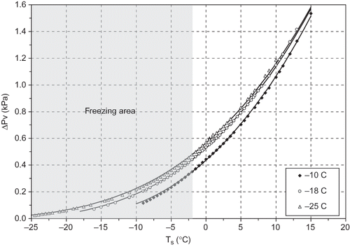
Figure 2 The surface temperature during the freezing process for the tested air temperatures (−10, −18, −25°C) and velocities (0.5, 1.0, 1.5, 2.0, 5.0 m^.s⁻¹).

where ΔP _v is the water vapour deficit in kPa and T _s is the surface temperature of the frozen produce in °C.

Estimation of the Heat and Mass Transfer Coefficients

The mean heat transfer coefficient (W m⁻² K⁻¹) depends on the velocity of the surrounding fluid, sample geometry, orientation, surface roughness, and other factors. Therefore, for most applications, must be determined experimentally.[21] The heat transfer coefficient for gas cross-flow over various cylinders was estimated by Hilpert[22] (Eq. 3a). The C and m values are given as 0.683 and 0.466 for 40 < Re < 4000 and 0.193 and 0.618 for 4000 < Re < 40,000, respectively.

(3a)

(3b)

(3c)

Estimation of was based on the geometry of the freezing sample as well the mean boundary layer temperature (also called ‘film temperature’), calculated as , where T _a is the air-freezing temperature and T _s the mean surface temperature estimated from the three thermocouples placed under the sample surface. The Pr value for the tested air conditions was taken as 0.71. The air density ρ, absolute viscosity μ, and thermal conductivity k _f were adopted from Massey,[23] Bayley et al.,[24] and Xanthopoulos,[25] respectively (shown in the appendix). Substituting the calculated parameters from Eqs. (3a) and (3b) into Eq. (3c), the mean heat transfer coefficient was estimated for the 15 experimental cases. Incropera and DeWitt[26] refer that the group of the empirical equations describing the heat and mass transfer equations in typical geometric bodies (spheres, cylinders, slabs, etc.) should be treated with caution since their empirical origin may produce great discrepancies.

Dincer and Genceli[16] conducted experiments on cucumber air cooling of similar geometry as the one used in the present experiments. The air velocities used by Dincer and Genceli[16] were of the same range as in the present experiment. Dincer and Genceli[16] calculated the Nu-Re correlation and the corresponding heat transfer coefficients. The derived Nu-Re equation was a modified Hilpert[22] correlation in which C = 1.264 and m = 0.449 for 100 < Re < 100,000. In a similar study, Dincer[2] developed a generic Nu-Re model. For this purpose, Dincer^[2] incorporated data from previous studies of cooling cylindrical products, such as banana and carrot. Dincer^[2] derived a new Nu-Re correlation in which C = 0.291 and m = 0.592 for 100 < Re < 100,000. The calculated values from the present study together with those calculated from Dincer and Genceli[16] and Dincer^[2] are presented in Fig. 4. Applying the Tukey HSD statistical test, it was found that values from Dincer^[2] and those from the present study were not significantly different (P ≤ 0.05). In Table 3, the estimated values from the present study are tabulated with the respective values from Dincer and Genceli^{[ 16 ]} and Dincer^[2] studies of air-cooling from 22 down to 2°C, for the same Re range. In Table 3, Dincer's^[2] values are closer to the values estimated in this study. The root mean square error (RMSE) of the values (shown in Table 3) from the present study and those from Dincer^[2] and Dincer and Genceli^{[ 16 ]} studies is 3.37 and 21.56, respectively. At this point, one has to consider that the estimated values from Dincer^[2] and from the present study are both based on generic models and, thus, exhibit a similar trend. The RMSE value of 3.37 lies within the experimental uncertainty range. The other pair comparison exhibits large RMS error. The noted errors can be originated from the estimation method of the heat transfer coefficients, the sample geometry (in Dincer^[2]the samples had 16.0 ± 0.5 cm height and 38.0 ± 1.0 mm diameter), the air conditions, etc. Based on the heat and mass transfer analogy, the mean mass transfer coefficient (m s⁻¹) was estimated from Eq. (4b)[26 27] and is tabulated in Table 3. The Sc value for the tested air conditions was taken as 0.6.

Table 3 The estimated , , and values for air-freezing of unpeeled cucumber (present experiment) compared to values from Dincer and Genceli^{[ 16 ]} and Dincer^[2] conducted experiments

			(W m^−2 K^−1)		(m s^−1)
V a (m s^−1)	Re	This study	Dincer & Genceli	Dincer	This study	This study
0.5	1460–1794	10.99 ± 0.16	—	—	8.98 ± 0.24	18.07 ± 0.38
1.0	2993–3474	15.14 ± 0.09	28.02 ± 1.20	18.22 ± 0.76	12.56 ± 0.25	24.71 ± 0.39
1.5	4323–5593	18.89 ± 0.17	37.21 ± 1.81	21.31 ± 0.97	15.42 ± 0.41	30.88 ± 1.18
2.0	6208–7382	22.23 ± 0.17	52.11 ± 3.02	26.56 ± 1.09	18.12 ± 0.31	37.86 ± 0.84
5.0	14,739–17,819	40.07 ± 0.15	—	—	32.40 ± 0.63	64.99 ± 1.64

(4a)

(4b)

Figure 4 Estimated values based on Hilpert correlation from the present experiment (points) compared to Dincer^[2] and Dincer and Genceli^{[ 16 ]} experiments for air-cooling of unpeeled cucumber.

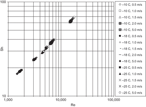
The mean number estimated from Eq. (4a) is tabulated in Table 3 and is presented in a log-log plot with Re in Fig. 5. The water vapour diffusivity D _f (m² s⁻¹) at the boundary layer was estimated from Kusuda,[28] as shown in Eq. (5):

(5)

Figure 5 Sherwood number variation with Re for air-freezing of unpeeled cucumber (present experiment).

In Table 3, it is shown that doubling the air velocity from 1.0 to 2.0 m^.s⁻¹ causes an increase of the by 47% in the present experiment, by 86% in Dincer and Genceli,^{[ 16 ]} and by 46% in Dincer^[2]. The Dincer and Genceli^{[ 16 ]} correlation is more sensitive to air conditions change. The respective increase is 44% while the increase is 53%. In Table A1 in the appendix, the estimated and the experimentally determined for the tested cases are tabulated analytically.

The Chilton-Colburn analogy is widely used for transverse flow around cylinders, flow through packed beds, and tubes at high Re.[29 30] In cases of low Re flow around objects, the two coefficients j _H and j _m are equal. Beyond the Re values, for which boundary layer separation occurs, the two coefficients become unequal. The Chilton-Colburn j-factor for heat and mass transfer were calculated by Eq. (6) and the mean values are presented in Table 4:

Table 4 The estimated values of , δ_θ ± std, δ_d ± std, and the experimental measured values of i _m ± std for air-freezing of unpeeled cucumber

V a (m s^−1)	Re	(j H , j M )^.10^3	10^3(m)	10^3(m)	.10^6(kg m^−2 s^−1)
0.5	1460–1794	13.20 ± 0.32	2.14 ± 0.03	20.96 ± 7.65	4.87 ± 3.0
1.0	2993–3474	9.19 ± 0.16	1.57 ± 0.02	15.06 ± 5.06	6.44 ± 3.58
1.5	4323–5593	7.54 ± 0.18	1.24 ± 0.02	10.56 ± 3.27	7.88 ± 4.56
2.0	6208–7382	6.64 ± 0.09	1.05 ± 0.02	7.07 ± 2.44	11.38 ± 5.40
5.0	14,739–17,819	4.76 ± 0.07	0.58 ± 0.01	5.46 ± 2.61	13.82 ± 9.13

(6)

Mass Loss Prediction

Based on the ‘Film Theory’, the thickness of the diffusive boundary layer is estimated from the viscous forces of the air stream, while the thickness of the thermal layer is estimated from the heat and mass transfer gradients.[29 31] Holman[27] reported that the thickness of the thermal boundary layer is significantly less than the diffusive layer. The heat flux (W m⁻²) is defined by Eq. (7):

(7)

where k _f is the air thermal conductivity, W m⁻¹ K⁻¹; is the mean thermal boundary layer, m; is the (convective) heat transfer coefficient, W m⁻² K⁻¹. The increases as decreases and decreases as airflow increases.[31] From Eq. (7), the values were calculated and presented in Table 4 for the five air velocities tested in this study.

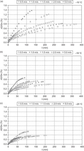
The mass loss during the experiments was regularly measured. From the estimated mass transfer rate and the sample surface area (Table 1), the mass flux rate i _m was experimentally estimated and tabulated in Table 4. The reduced mass loss (G _o - G _i /G _o ) was also calculated and presented in Figs. 6a–6c. Freezing at −25°C gave the smallest mass loss, probably due to faster ice formation in the outer layer of the produce. The mass loss increased as the freezing temperature was raised from −25 to −18 and −10°C, respectively. The freezing air velocity, affected in a smaller degree the mass loss as the air temperature was lowered, and this can be explained from the mass loss curves for the different air velocities, which are quite close at −18°C and almost coincide at −25°C.

Figure 6 The reduced mass loss (%) during the freezing process for the tested air temperatures (−10, −18, −25°C) and velocities (0.5, 1.0, 1.5, 2.0, 5.0 m^.s⁻¹).

From the ‘Film Theory’, the mass flux rate i _m due to water diffusion from the sample surface to the air freezing stream through the stagnant (diffusive) boundary layer^{[ 29,30 ]} is described by Eq. (8). In the diffusive boundary layer , the water vapour pressure gradient is the driving force of the water vapour diffusion.

(8)

where is the mass flux rate, kg m⁻² s⁻¹; R _v is the water vapour gas constant (461.52 J kg⁻¹ K⁻¹); is the partial water vapour pressure of the surface and air, respectively, Pa; and is the mean diffusive boundary layer, m.

Solving Eq. (8) with respect to , the weighted mean values were calculated and tabulated in Table 4. As the sublimation/evaporation progress, the driving force is reduced due to the movement of the sublimation front to the geometric centre of the freezing produce. The sublimed water vapour from the inner tissues to the surface encounters increased resistance as the freezing time progresses.

CONCLUSIONS

The heat and mass transfer coefficients of freezing unpeeled cucumber were estimated implementing the Hilpert equation. The calculations were based on the surface temperature of the samples subjected to five air-freezing velocities and three low air-temperatures. The estimated , were compared with the respective values estimated from Dincer and Dincer and Genceli. The RMSE of the values (Table 3) from the present study and those estimated from the Dincer study was 3.37, which is considered within the experimental uncertainty range. The Chilton-Colburn j-factors of heat and mass transfer and the mean diffusive and thermal boundary layers were also estimated and presented with the respective values. The i _m values were calculated and presented graphically. The smallest mass loss was estimated at −25°C, in which air velocity in all the tested cases did not affected significantly mass loss probably due to the fast formation of a protective surface ice layer that restricted water losses.

NOMENCLATURE

a,b,c	=	coefficients of Eq. (2)
C,m	=	coefficients of Eq. (3)
D	=	diameter (m)
L	=	length (cm)
S	=	sample surface area (cm2)
G o	=	initial sample weight (g)
G i	=	sample weight in time i (g)
D f	=	diffusivity of water vapour in the air at T f (m2 s−1)
	=	mean convection heat transfer coefficient (W m−2 K−1)
j H , j m	=	Chilton-Colburn j-factors of heat and mass transfer
	=	density of mass flow (flux) (kg m−2 s−1)
k f	=	thermal conductivity of the air at T f (W m−1 K−1)
	=	mean mass transfer coefficient (m s−1)
	=	mean Nusselt number
Pr	=	Prandtl number
P s	=	saturation water vapour pressure (Pa)
P v	=	partial water vapour pressure (Pa)
	=	partial water vapour pressure in the air (Pa)
	=	heat flux (W m−2)
	=	adjusted coefficient of determination
Re	=	Reynolds number
RMSE	=	root mean square error
R v	=	water vapour gas constant (461.52 J kg−1 K−1)
Sc	=	Schmidt number
SEE	=	standard error of estimate
	=	mean Sherwood number
T a	=	air temperature (°C)
T f	=	mean boundary layer temperature [film temperature] (K)
T s	=	sample surface temperature (°C)
V a	=	air velocity (m s−1)
ΔP v	=	water vapour deficit of the freezing air (Pa)

Greeks

	=	mean thermal boundary layer (m)
	=	mean diffusive boundary layer (m)
ρ	=	air density (kg m−3)
μ	=	absolute viscosity of air (N s m−2 or kg m−1 s−1)

APPENDIX

Table A1 The calculated , , , and values and the experimentally measured values for all the tested cases

T(°C)	V(m^.s^−1)		(W m^−2 K^−1)		(m s^−1)	(kg m^−2 s^−1)
−10	0.5	1526 ± 28	11.19 ± 0.007	17.54 ± 0.15	9.24 ± 0.005	5.29 ± 3.10
	1.0	3130 ± 57	15.25 ± 0.009	24.51 ± 0.21	12.60 ± 0.007	6.68 ± 3.94
	1.5	4541 ± 80	19.10 ± 0.04	29.63 ± 0.33	15.78 ± 0.03	8.67 ± 5.33
	2.0	6498 ± 109	22.17 ± 0.04	36.98 ± 0.38	18.32 ± 0.03	13.66 ± 5.33
	5.0	15,337 ± 249	40.00 ± 0.07	62.86 ± 0.63	33.05 ± 0.06	22.18 ± 10.62
−18	0.5	1674 ± 27	10.82 ± 0.005	18.31 ± 0.14	8.67 ± 0.004	4.91 ± 3.36
	1.0	3300 ± 60	15.04 ± 0.01	25.12 ± 0.21	12.05 ± 0.006	6.60 ± 3.64
	1.5	4917 ± 85	18.81 ± 0.04	31.12 ± 0.33	15.07 ± 0.03	7.64 ± 3.81
	2.0	6923 ± 118	22.08 ± 0.05	38.45 ± 0.40	17.69 ± 0.03	10.02 ± 4.91
	5.0	16,084 ± 301	39.98 ± 0.09	64.73 ± 0.75	32.03 ± 0.07	14.99 ± 6.95
−25	0.5	1665 ± 39	11.02 ± 0.01	18.27 ± 0.19	8.60 ± 0.004	4.38 ± 2.46
	1.0	3092 ± 46	15.16 ± 0.01	24.38 ± 0.17	11.83 ± 0.005	5.92 ± 3.10
	1.5	5236 ± 138	18.73 ± 0.06	32.35 ± 0.53	14.61 ± 0.05	7.04 ± 4.17
	2.0	6872 ± 204	22.46 ± 0.09	38.27 ± 0.70	17.52 ± 0.06	10.15 ± 5.27
	5.0	16,764 ± 401	40.19 ± 0.13	66.41 ± 0.98	31.35 ± 0.09	8.18 ± 4.96

•	The density[ 23 ] ρ of air is calculated as: where P a  = atmospheric pressure, taken as 101.3.kPa; R = specific air constant, J kg−1 K−1; T a  = air temperature in °C; ρ a  = air density, kg m−3.
•	Sutherland's law[24] describes the absolute viscosity μ and is given as: where μ = air absolute viscosity, kg m−1.s−1 (or N.s m−2); S 1 = 1.46 10−6; and S 2 = 110.
•	The air conductivity[25] k a is given as: where k a  = air conductivity, W m−1 K−1; c 1 = 0.024; c 2 = 0.791 10−4; c 3 = −0.329 10−7; T = air temperature, °C.

REFERENCES

- Heldman , D.R. 1975 . Food Process Engineering , Westport , CT : AVI Publishing Co .
- Dincer , I. 1994 . Development of new effective Nusselt-Reynolds correlations for air-cooling of spherical and cylindrical products . International Journal of Heat and Mass Transfer , 37 ( 17 ) : 2781 – 2787 .
- Clary , B.L. , Nelson , G.L. and Smith , R.E. 1968 . Heat transfer from hams during freezing by low-temperature air . Transactions of the ASAE , 11 ( 4 ) : 496 – 499 .
- Cleland , A.C. and Earle , R.L. 1976 . A new method for prediction of surface heat transfer coefficients in freezing . Bulletins of International Institute of Refrigeration , 1 : 361 – 368 .
- Flores , E.S. and Mascheroni , R.H. 1988 . Determination of heat transfer coefficients for continuous belt freezers . Journal of Food Science , 53 ( 6 ) : 1872 – 1876 .
- Daudin , J.D. and Swain , M.V.L. 1990 . Heat and mass transfer in chilling and storage of meat . Journal of Food Engineering , 12 ( 2 ) : 95 – 115 .
- Khairullah , A. and Singh , R.P. 1991 . Optimization of fixed and fluidized bed freezing processes . International Journal of Refrigeration , 14 ( 3 ) : 176 – 181 .
- Kondjoyan , A. and Daudin , J.D. 1997 . Heat and mass transfer coefficients at the surface of a pork hindquarter . Journal of Food Engineering , 32 ( 2 ) : 225 – 240 .
- Delgado , A.E. and Sun , D.W. 2001 . Heat and mass transfer models for predicting freezing processes—A review . Journal of Food Engineering , 47 : 157 – 174 .
- Krokida , M.K. , Zogzas , N.P. and Maroulis , Z.B. 2001 . Mass transfer coefficient in food processing: Compilation of literature data . International Journal of Food Properties , 4 ( 3 ) : 373 – 382 .
- Zogzas , N.P. , Krokida , M.K. , Michailidis , P.A. and Maroulis , Z.B. 2002 . Literature data of heat transfer coefficients in food processing . International Journal of Food Properties , 5 ( 2 ) : 391 – 417 .
- Wang , L. and Sun , D.W. 2003 . Recent developments in numerical modelling of heating and cooling processes in the food industry—A review . Trends in Food Science and Technology , 14 : 408 – 423 .
- Pham , Q.T. 2006 . Modelling heat and mass transfer in frozen foods: A review . International Journal of Refrigeration , 29 : 876 – 888 .
- Kondjoyan , A. 2006 . A review on surface heat and mass transfer coefficients during air chilling and storage of food products . International Journal of Refrigeration , 29 : 863 – 875 .
- Statgraphics Plus 5.1 . 2001 . Online Manual , Warrenton, Virginia , , USA : Statistical Graphics Inc .
- Dincer , I. and Genceli , O.F. 1994 . Cooling process and heat transfer parameters of cylindrical products cooled both in water and in air . International Journal of Heat and Mass Transfer , 37 ( 4 ) : 625 – 633 .
- Mason , R.L. , Gunst , R.F and Hess , J.L. 2003 . Statistical Design and Analysis of Experiments: With Applications to Engineering and Science , 2nd , 196 – 213 . New Jersey, USA : Wiley-Interscience .
- Wexler , A. and Hyland , R.W. 1980 . A formulation for the thermodynamic properties of the saturated pure ordinary water-substance from 173.15 to 473.15 K , ASHRAE Research Project RP216 .
- Leniger , H.A. and Beverloo , W.A. 1975 . Food Process Engineering; D. Reidel . Dordrecht, Netherlands , : 351 – 398 .
- Anonymous . 1986 . Recommendations for the Processing and Handling of Frozen Foods , 3rd , Paris , , France : I.I.R .
- ASHRA , E. 1998 . Thermal Properties of Foods , Atlanta, GA , , USA : Handbook of Refrigeration, American Society of Heating, Refrigeration and Air Conditioning Engineers, Inc .
- Hilpert , R. 1933 . “ Wärmeabgade von geheizen Drahten und Rohren ” . In Forsch, Geb. Ingenieurwes , 7th , Edited by: Holman , J.P. Heat Transfer . Vol. 4 , 215 NY , , USA : McGraw Hill . 1989, 333
- Massey , B.S. 1997 . Mechanics of Fluids , 6th , 1 – 26 . London : Chapman & Hall .
- Bayley , F.J. , Owen , J.M. and Turner , A.B. 1972 . Heat Transfer , 1st , New York : Thomas Nelson and Sons .
- Xanthopoulos , G. 2002 . Simulation of heat and mass transfer and biological changes in a grain store , Newcastle , , UK : Ph.D. Thesis, University of Newcastle upon Tyne .
- Incropera , F.P. and DeWitt , D.P. 1996 . Introduction to Heat Transfer , 3rd , New York : Wiley .
- Holman , J.P. 1989 . Heat Transfer , 7th , New York : McGraw Hill .
- Kusuda , T. 1965 . “ Calculation of the temperature of a flat-plate wet surface under adiabatic conditions with respect to the Lewis relation ” . In Humidity and Moisture: Measurement and Control in Science and Industry , Edited by: Ruskin , R.E . Vol. I , 16 New York : Reinhold Publishing .
- Bird , R.B. , Stewart , W.E. and Lightfoot , E.N. 1960 . Transport Phenomena , 2nd , New York : Wiley .
- Treyball , R.E. 1980 . Mass Transfer Operations , 3rd , New York : McGraw-Hill .
- Pabis , S. , Jayas , D.S. and Cenkowski , S. 1998 . Grain Drying: Theory and Practice , 1st , 28 – 29 . New York : Wiley .