Thermal properties determination of a cylindrical product during its cooling: two-dimensional numerical model and uncertainty

ABSTRACT

In this article, a two-dimensional model is proposed to determine thermal diffusivity and convective heat transfer coefficient, providing the average values, their uncertainties and the covariance matrix referring to these parameters for a product with cylindrical geometry during its cooling. The proposed model used a two-dimensional numerical solution of the diffusion equation for the direct problem; an experimental dataset referring to the cooling kinetics in the center of the product and an optimizer program based on the Levenberg-Marquardt algorithm for the inverse problem. The model was used with success to determine the thermal properties, their uncertainties and the covariance matrix of a cucumber during its cooling. The obtained results allowed establishing a confidence band that made it possible to graphically evaluate the precision of a new simulation for a cucumber with different dimensions.

KEYWORDS:

• Thermal diffusivity
• convective heat transfer coefficient
• uncertainties
• covariance matrix
• numerical solution
• cooling

Introduction

In order to increase the post-harvest life of agricultural products, their processing is usually carried out, often involving the simultaneous heat and mass transfer, as in the case of drying.^[1–3] Other types of processing involve simple heat transfer, such as pasteurization^[4–6], cooling^[7–11], and also freezing.^[12,13] To simulate all these processes, and consequently to obtain information such as their duration, as well as the energy required, among others, it is necessary to know the initial and final temperatures of the product, its geometry, and its dimensions, as well as its thermophysical properties. To determine these properties during a transient state, various optimization techniques can be used such as the concept of lag factor^[7] or the similar “slope method”.^[10] This technique uses a single term representing the analytical solution of the partial differential equation which describes the physical phenomenon and it disregards, by graphical inspection with the use of logarithm, the first experimental points, in such a way that this single term is sufficient to describe well the phenomenon. However, if many experimental points are disregarded, statistical information is lost. Thus, Silva et al.^[8] proposed an algorithm for the optimal determination of the number of points to be disregarded. To this technique of determination of parameters, the authors gave the name of “Optimal Removal of Experimental Points – OREP”, and such technique makes it possible to generate good results for the thermal properties during the transient state of a process.

Some methods (so-called “robust”), which determine parameters of partial differential equations through successive trials and an experimental dataset, are also available in the literature.^[3,6] However, for the specific case of heat transfer, in many works available in the literature the values of the thermal properties are determined without their uncertainties being known, as well as the covariance between such values. Thus, the use of the values of such properties to simulate pasteurization, cooling, and freezing are compromised due to the lack of information on the precision of the results obtained.

Le Niliot, and Lefevre^[14] and also Mariani et al.^[12], in order to determine the uncertainties of thermal properties, proposed to perform 100 numerical simulations where the measurements are disrupted with 100 different Gaussian distributions (with zero mean and standard deviation obtained from the simulation using the parameters originally determined). Thus, the uncertainties were obtained by performing the statistical treatment of the 100 values for each parameter. Da Silva and Silva^[9] have also used this method to determine the covariance matrix related to the thermal diffusivity and the convective heat transfer coefficient during cucumber cooling. However, this method, despite being able to determine the uncertainties of parameters and the covariance matrix, is very slow due to the number of simulations required. Thus, this method has usually been employed for one-dimensional geometries, whose simulations are generally faster than those for two- and three-dimensional ones.

Other techniques to determine parameters of differential equation (and their uncertainties) using experimental dataset have also been found in the literature in recent years.^[15–17] However, the necessary codes to do it (such as OptiPa, SBtoolbox2, and AMIGO2) are usually made available (or developed) for MATLAB environment. In the year 2017, the first two authors of the present article developed the program LS Optimizer (Version 6.2, 2018, http://zeus.df.ufcg.edu.br/labfit/LS.htm), to be installed directly on Windows platform. This free software, based on the Levenberg-Marquardt algorithm^[18–20], is very fast to determine parameters of a differential equation using experimental data. Thus, this software makes it possible to use two- and three-dimensional models in order to determine thermal properties during a transient state, with no need for a specific computational environment. In this context, the objectives of this article are defined below.

The main objective of this article was to propose a two-dimensional numerical model to determine thermal properties (their uncertainties and the covariance matrix) of products with cylindrical geometry, using an experimental dataset obtained during their cooling. Thus, the obtained values can be used to predict new cooling curves for the same product, but with different dimensions. As an application, the model was used to determine the thermal diffusivity and the convective heat transfer coefficient (their uncertainties and covariance matrix) for a cucumber during its cooling process.

Materials and methods

Heat conduction in cylindrical geometry

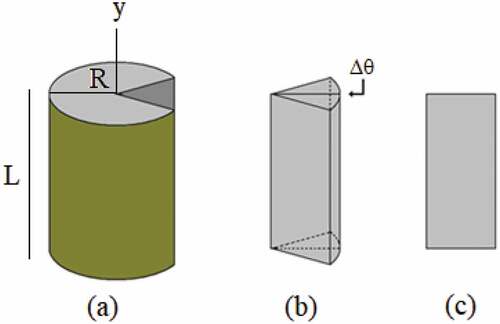
If a heat conduction process in a cylindrical domain (with radius R and height L) is symmetric with respect to the y-axis, as shown in Figure 1a, the diffusion equation to describe the unsteady state process is given by:

(1) $\frac{\mathrm{\partial }(\rho c_{p}T)}{\mathrm{\partial }t}=\frac{1}{r}\frac{\mathrm{\partial }}{\mathrm{\partial }r}\left(rk\frac{\mathrm{\partial }T}{\mathrm{\partial }r}\right)+\frac{\mathrm{\partial }}{\mathrm{\partial }y}\left(k\frac{\mathrm{\partial }T}{\mathrm{\partial }y}\right)$(1)

Figure 1. (a) Finite cylinder with radius R and height L; (b) symmetrical slice defined by the angle Δθ; (c) Rectangle dividing the slice in the middle where a two-dimensional grid will be defined

where $\rho$ (kg m⁻³) is the density, $c_p$ (J kg⁻¹ K⁻¹) is the specific heat, $T$ (K) is the temperature, $k$ (W m⁻¹ K⁻¹) is the thermal conductivity, $t$ (s) is the time and $r$(m) and $y$(m) are the coordinates of position. For agricultural products, a cooling process usually involves a temperature variation of about 20°C or less. Thus, the following assumptions can be accepted to describe cooling of cylindrical agricultural products: (1) the thermophysical parameters can be considered as constant during the process; (2) for some of these products, it can be assumed that the cylindrical medium is homogeneous and isotropic; (3) for the proposed model, it was considered that heat transfer can be described only by conduction. Thus, the thermal diffusivity $\alpha$ (m² s⁻¹), defined below, should be considered as “apparent”:

(2) $\alpha =\frac{k}{\rho c_p}$(2)

Since the thermophysical properties were considered as constant, Equation (1)(1) $\frac{\mathrm{\partial }(\rho c_{p}T)}{\mathrm{\partial }t}=\frac{1}{r}\frac{\mathrm{\partial }}{\mathrm{\partial }r}\left(rk\frac{\mathrm{\partial }T}{\mathrm{\partial }r}\right)+\frac{\mathrm{\partial }}{\mathrm{\partial }y}\left(k\frac{\mathrm{\partial }T}{\mathrm{\partial }y}\right)$(1) can be divided by $\rho c_p$, and rewritten as:

(3) $\frac{\mathrm{\partial }(T)}{\mathrm{\partial }t}=\frac{1}{r}\frac{\mathrm{\partial }}{\mathrm{\partial }r}\left(r\alpha \frac{\mathrm{\partial }T}{\mathrm{\partial }r}\right)+\frac{\mathrm{\partial }}{\mathrm{\partial }y}\left(\alpha \frac{\mathrm{\partial }T}{\mathrm{\partial }y}\right)$(3)

Direct problem: solver

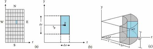
A solver for Equation (3)(3) $\frac{\mathrm{\partial }(T)}{\mathrm{\partial }t}=\frac{1}{r}\frac{\mathrm{\partial }}{\mathrm{\partial }r}\left(r\alpha \frac{\mathrm{\partial }T}{\mathrm{\partial }r}\right)+\frac{\mathrm{\partial }}{\mathrm{\partial }y}\left(\alpha \frac{\mathrm{\partial }T}{\mathrm{\partial }y}\right)$(3) was obtained using the Finite Volume Method with a fully implicit formulation.^[21] Several authors have shown that the diffusion equation for the cylinder has unique analytical solution.^[8,11] However, for the numerical solution proposed, the fully implicit formulation was chosen because it is unconditionally stable.^[9] A numerical solution was chosen because such a solution can be obtained even if the thermal properties and the dimensions of the domain are variable along the process. On the other hand, considering a symmetric heat conduction with respect to the y-axis, only the piece shown in Figure 1b can be considered to solve the diffusion equation. Thus, a grid can be created in the rectangle presented in Figure 1c. As a result, a two-dimensional uniform grid can be obtained, as shown in Figure 2a. In addition, Figure 2b shows a rectangular element of the grid, whose sides are $\mathrm{\Delta }r$ and $\mathrm{\Delta }y$. A revolution of this rectangular element in $\mathrm{\Delta }\theta$ radians around the y-axis shows the control volume given in Figure 2c: $\mathrm{\Delta }V=\mathrm{\Delta }\theta r_P\mathrm{\Delta }r\mathrm{\Delta }y$, where $r_P$ defines the radial position of the nodal point P of the rectangular element.

Figure 2. (a) Two-dimensional grid for the cylindrical geometry with boundaries north (N), south (S), west (W) and east (E); (b) Element of the two-dimensional grid highlighting the nodal point P; (c) Control volume for the cylindrical geometry

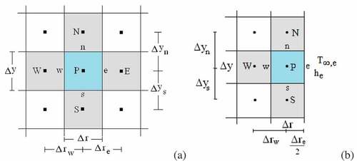
By observing Figure 2a, it is possible to conclude that, for the two-dimensional domain, there are nine types of control volumes: internal (no contact with external medium), north, north-east, south, south-east, east, north-west, south-west, and west. Due to the radial symmetry, it is observed that the last three types of control volumes have flux zero at the west boundary. Integrating Equation (3)(3) $\frac{\mathrm{\partial }(T)}{\mathrm{\partial }t}=\frac{1}{r}\frac{\mathrm{\partial }}{\mathrm{\partial }r}\left(r\alpha \frac{\mathrm{\partial }T}{\mathrm{\partial }r}\right)+\frac{\mathrm{\partial }}{\mathrm{\partial }y}\left(\alpha \frac{\mathrm{\partial }T}{\mathrm{\partial }y}\right)$(3) in space ($\mathrm{\Delta }\theta r_P\mathrm{\Delta }r\mathrm{\Delta }y$) and time ($\mathrm{\Delta }t$) for a given control volume, after the simplifications, yields:

(4) $\frac{T_P-T_P^0}{\mathrm{\Delta }t}{r}_p\mathrm{\Delta }r\mathrm{\Delta }y=\left(r_e{\alpha }_e\frac{\mathrm{\partial }T}{\mathrm{\partial }r}{|}_e-r_w{\alpha }_w\frac{\mathrm{\partial }T}{\mathrm{\partial }r}{|}_w\right)\mathrm{\Delta }y+\left({\alpha }_n\frac{\mathrm{\partial }T}{\mathrm{\partial }y}{|}_n-{\alpha }_s\frac{\mathrm{\partial }T}{\mathrm{\partial }y}{|}_s\right)\hspace{0.17em}{r}_p\mathrm{\Delta }r$(4)

where the superscript 0 means “former time” t, and its absence means “current time”, t+∆t. The subscripts “e”, “w”, “n”, “s” are, respectively, east, west, north, and south interfaces, while P is the nodal point of the control volume.

Internal control volume

A control volume is defined as “internal” if it has neighbors to the north, south, east, and west. As an example, an internal control volume and its neighbors to the north, south, east, and west are shown in Figure 3a. For this type of control volume, substituting the derivatives of Equation 4(4) $\frac{T_P-T_P^0}{\mathrm{\Delta }t}{r}_p\mathrm{\Delta }r\mathrm{\Delta }y=\left(r_e{\alpha }_e\frac{\mathrm{\partial }T}{\mathrm{\partial }r}{|}_e-r_w{\alpha }_w\frac{\mathrm{\partial }T}{\mathrm{\partial }r}{|}_w\right)\mathrm{\Delta }y+\left({\alpha }_n\frac{\mathrm{\partial }T}{\mathrm{\partial }y}{|}_n-{\alpha }_s\frac{\mathrm{\partial }T}{\mathrm{\partial }y}{|}_s\right)\hspace{0.17em}{r}_p\mathrm{\Delta }r$(4) by numerical approximations of first-order yields:

(5) $A_P{T}_P=A_e{T}_E+A_w{T}_W+A_n{T}_N+A_s{T}_S+B$(5)

Figure 3. (a) Internal control volume, nodal point P and neighbors to the north (N), south (S), east (E) and west (W); (b) Control volume P at the east boundary and its neighbors

where:

(6) $A_P=\frac{r_P\mathrm{\Delta }r\mathrm{\Delta }y}{\mathrm{\Delta }t}+r_e{\alpha }_e^{\hspace{0.17em}}\frac{\mathrm{\Delta }y}{\mathrm{\Delta }r}+r_w{\alpha }_w^{\hspace{0.17em}}\frac{\mathrm{\Delta }y}{\mathrm{\Delta }r}+r_p{\alpha }_n^{\hspace{0.17em}}\frac{\mathrm{\Delta }r}{\mathrm{\Delta }y}+r_P{\alpha }_s^{\hspace{0.17em}}\frac{\mathrm{\Delta }r}{\mathrm{\Delta }y}$(6)

(7) $A_e=r_e{\alpha }_e^{\hspace{0.17em}}\frac{\mathrm{\Delta }y}{\mathrm{\Delta }r}$(7)

(8) $A_w=r_w{\alpha }_w^{\hspace{0.17em}}\frac{\mathrm{\Delta }y}{\mathrm{\Delta }r}$(8)

(9) $A_n=r_P{\alpha }_n^{\hspace{0.17em}}\frac{\mathrm{\Delta }r}{\mathrm{\Delta }y}$(9)

(10) $A_s=r_P{\alpha }_s^{\hspace{0.17em}}\frac{\mathrm{\Delta }r}{\mathrm{\Delta }y}$(10)

(11) $B=\frac{r_p\mathrm{\Delta }r\mathrm{\Delta }y}{\mathrm{\Delta }t}{T}_P^0$(11)

East boundary

A control volume P at the east boundary and its neighbors to the north (N), south (S), and west (W) are shown in Figure 3b. In this figure, the symbols denoted by $T_{\mathrm{\infty },e}$ (K) and $h_e$ (ms⁻¹) represent the equilibrium temperature and the convective heat transfer coefficient at the east boundary, respectively. Thus, the following result for the discretization is obtained:

(12) $A_P{T}_P=A_w{T}_W+A_n{T}_N+A_s{T}_S+B$(12)

The coefficients A_w, A_n, and A_s of Equation 12(12) $A_P{T}_P=A_w{T}_W+A_n{T}_N+A_s{T}_S+B$(12) are given by Equations 8(8) $A_w=r_w{\alpha }_w^{\hspace{0.17em}}\frac{\mathrm{\Delta }y}{\mathrm{\Delta }r}$(8) –10(10) $A_s=r_P{\alpha }_s^{\hspace{0.17em}}\frac{\mathrm{\Delta }r}{\mathrm{\Delta }y}$(10) , respectively. The coefficients A_P and B are given by:

(13) $A_P=\frac{r_P\mathrm{\Delta }r\mathrm{\Delta }y}{\mathrm{\Delta }t}+\frac{r_e\mathrm{\Delta }y}{\frac{1}{h_e}+\frac{\mathrm{\Delta }r}{2{\alpha }_e^{\hspace{0.17em}}}}+r_w{\alpha }_w^{\hspace{0.17em}}\frac{\mathrm{\Delta }y}{\mathrm{\Delta }r}+r_p{\alpha }_n^{\hspace{0.17em}}\frac{\mathrm{\Delta }r}{\mathrm{\Delta }y}+r_P{\alpha }_s^{\hspace{0.17em}}\frac{\mathrm{\Delta }r}{\mathrm{\Delta }y}$(13)

and

(14) $B=\frac{r_P\mathrm{\Delta }r\mathrm{\Delta }y}{\mathrm{\Delta }t}{T}_P^0+\frac{r_e\mathrm{\Delta }y}{\frac{1}{h_e}+\frac{\mathrm{\Delta }r}{2{\alpha }_e^{\hspace{0.17em}}}}{T}_{\mathrm{\infty },e}$(14)

As an additional information, this numerical solution has been previously validated using a two-dimensional analytical solution presented in Ref.^[11] On the other hand, the last results were obtained by imposing equal diffusive and convective fluxes at the east interface of the control volume with nodal point P (see Figure 3b): $-{\alpha }_e\mathrm{\partial }T/\mathrm{\partial }r\left|{ }_{{ }_{{ }_e}}\right.=h_e(T_e-T_{\mathrm{\infty },e})$. This equation defines the boundary condition of the third kind for the east side (subscript “e”). In this last equation, $T_e$ (K) is the temperature at the east boundary, while $T_{\mathrm{\infty },e}$ is the cooling temperature at the east side of the medium. On the other hand, the heat transfer coefficient $h_{He}$ (W m⁻² K⁻¹) and $h_e$ are related as follows:

(15) $h_e=\frac{h_{He}}{\rho c_p}$(15)

The same discretization procedure mentioned above can be used to discretize the other seven types of control volumes. Thus, a system of equations for each time step is obtained with the Equations 5(5) $A_P{T}_P=A_e{T}_E+A_w{T}_W+A_n{T}_N+A_s{T}_S+B$(5) ,12(12) $A_P{T}_P=A_w{T}_W+A_n{T}_N+A_s{T}_S+B$(12) and other similar equations, and this system can be solved, for instance, by the Gauss–Seidel method^[22], with a convergence tolerance of 1 ×10⁻⁸. Specifically in this article, because the thermal properties are considered constant, for each control volume the following equality is observed: ${\alpha }_e^{\hspace{0.17em}}={\alpha }_w^{\hspace{0.17em}}={\alpha }_n^{\hspace{0.17em}}={\alpha }_s^{\hspace{0.17em}}=\alpha$. Also, at the boundaries of the rectangular grid (Figure 2a) the following equality can be written: $h_e^{\hspace{0.17em}}=h_n^{\hspace{0.17em}}=h_s^{\hspace{0.17em}}=h$. On the other hand, on the whole west side, due to the radial symmetry, the heat flux is zero.

The solver for the simulation of heat transfer at a specified point within the finite cylinder was created in FORTRAN. This solver was created in Compaq Visual Fortran Professional Studio, Edition V. 6.6.0, using a programming language option called QuickWin Application.

Inverse problem: parameter determination

Thermal diffusivity $\alpha$ and convective heat transfer coefficient $h$ were determined using LS Optimizer Software, developed by the first and second authors of this article. The program is freely available at http://zeus.df.ufcg.edu.br/labfit/LS.htm, and it is intended for the solution of inverse problems, determining parameters of differential equations and other types of complex functions for a specified experimental dataset. The Levenberg-Marquardt algorithm^[18–20] is used by LS Optimizer, which executes the solver provided by the user in order to determine the parameters that allow a simulation as close as possible to the experimental dataset. The software’s Help Menu explains how to add a few lines in the solver’s original code, allowing the reading of information provided by LS, and vice-versa, through text files.

According to the information available in the LS Optimizer manual, as long as the solver for the direct problem and the experimental dataset are provided, this optimization software executes the solver in order to obtain the necessary information for the determination of parameters, using the statistical indicator chi-square as the objective function. As mentioned by Da Silva et al.^[11], through the experimental ($T_i^{exp}$) and simulated ($T_i^{sim}$) values, the optimizer program iteratively determines corrections for h and α, and calculates the chi-square referring to each simulation through the expression ${\chi }^2=\sum {\left(T_i^{exp}-T_i^{sim}\right)}^2/{\sigma }_{T_i}^2$, until it reaches a minimum value. If the uncertainties of the experimental points (σ_Ti) are not known at first, it is possible to determine the standard deviation associated with the optimization process, given by $\sigma =\sqrt{{\sum }^{{\left(T_i^{exp}-T_i^{sim}\right)}^2}/(N-n)}$, in which (N-n) is the number of degrees of freedom. Hence, at the end of the iterative process, one can impose ${\sigma }_{T_i}=\sigma$ and recalculate the covariance matrix, which provides the uncertainties of the parameters and the correlation between them. Thus, starting from initial values α₀ and h₀, the optimizer corrects these parameters iteratively up to convergence and, in the end, LS Optimizer delivers the optimal values for α and h, their uncertainties, the covariance matrix, and graphs.

In this article, the initial values for the parameters to be determined were established as α₀ = 1 x 10⁻⁷ m² s⁻¹ and h₀ = 1 x 10⁻⁶ m s⁻¹. If the LS user considers that the initial values are not so reasonable, the corrections calculated by the optimizer can produce the divergence of the iterative process that obtains the parameters. Due to that, the optimizer has a resource called “split first corrections into…”. In this optimization process, using this resource, the first corrections of the parameters were divided into 40 parts. Therefore, only 1/40 of the values calculated were used to correct the parameters in the first corrections.

Experimental dataset

The model proposed in this article to determine thermal properties of a cylindrical product involves: (1) A solver for the direct problem, presented in Section 2.2; (2) An optimizer program for the inverse problem, presented in Section 2.3; and (3) An experimental dataset referring to the cooling kinetics at a specified point within the cylindrical domain.

Silva et al.^[8] have proposed a one-dimensional model in which the thermal properties are determined by the fitting of only the first term of the series representing the analytical solution of the one-dimensional diffusion equation. Due to this proposal, the first experimental points must be disregarded to perform the curve fitting. Then, the authors have proposed an algorithm to determine the number of the optimal removal of experimental points, in order to maintain as much statistical information as possible. This model was applied to the cooling of cucumbers under natural convection and, in the present article, for comparison purposes, the same experimental dataset will be used. The cucumber used in the experiment has a radius R = 0.019 m and a height L = 0.160 m. During the experiment, the mass loss was considered to be negligible. The moisture content of the product was X = 0.96 (w.b.), and its initial temperature was $T_{{ }_0}=22.0{}^{\mathrm{o}}\mathrm{C}$. The temperature of the cooling air was $T_{{ }_{\mathrm{\infty }}}=4.0{}^{\mathrm{o}}\mathrm{C}$, and its velocity was kept at 2 m s⁻¹, with a relative humidity of 80%. The cooling kinetics was determined through a thermocouple placed in the center of the product (r = 0 and y = 0), and the temperature was measured at regular intervals of time, totaling 37 experimental points. In order to determine the thermal properties, the dataset was written in the dimensionless form:

(16) $T^{\ast }=\frac{T-T_{\mathrm{\infty }}}{T_0-T_{\mathrm{\infty }}}$(16)

Results and discussion

In order to solve the direct problem, a 40 × 100 grid was used and the cooling duration was divided into 1000 time steps. For these values, it was possible to observe that the first six significant figures of each temperature obtained are independent of new refinements for the grid and time.

Results

After convergence, LS Optimizer provided the values of the parameters, and also the factor to multiply the uncertainties so that the confidence interval is 95.4% (in the present case, it was obtained: factor = 2.04). Thus, the final results for the thermal properties and their uncertainties are given in Table 1.

Table 1. Thermal properties (thermal diffusivity, thermal conductivity, convective heat transfer coefficient, heat transfer coefficient) determined by the proposed model and by Silva et al.^[8]

Thermal property	Proposed model	Silva et al.^[Citation8]
α (m^2 s^−1)	(1.48 ± 0.12)×10^−7	1.47 × 10^−7
k (W m^−1 K^−1)	0.60 ± 0.05	–
h (m s^−1)	(6.35 ± 0.25)×10^−6	6.39 × 10^−6
hH (W m^−2 K^−1)	25.5 ± 1.0	–

It is interesting to observe that the thermal conductivity k was determined from Equation 2(2) $\alpha =\frac{k}{\rho c_p}$(2) , and the heat transfer coefficient h_H was calculated using Equation 15(15) $h_e=\frac{h_{He}}{\rho c_p}$(15) . For that, the specific heat was estimated from the expression^[23,24]: $c_p=1.381+2.930X(kJk{g}^{-1}{K}^{-1})$. The cucumber density value used in the present article was determined by Fasina and Fleming^[25] as: ρ = 959 kg m⁻³. It is interesting to observe that the value obtained for k agrees with the value obtained by the empirical equation provided in Ref.^[23] for the thermal conductivity (k = 0.148 +0.493X): k = 0.62 W m⁻¹ K⁻¹. The discrepancy between the two values is only 3%.

Another result provided by LS Optimizer is the covariance matrix, given by:,

$cov=\left[\begin{array}{c}3.672\times {10}^{-17}-7.021\times {10}^{-16}\\ -7.021\times {10}^{-16}1.491\times {10}^{-14}\end{array}\right]$

indicating a correlation coefficient between α and h of −0.9489 and, even with this high negative correlation, the iterative process has converged. With the results obtained for α and h, the cooling kinetics of the cucumber is shown in Figure 4.

Figure 4. Cooling kinetics of the cucumber

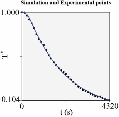
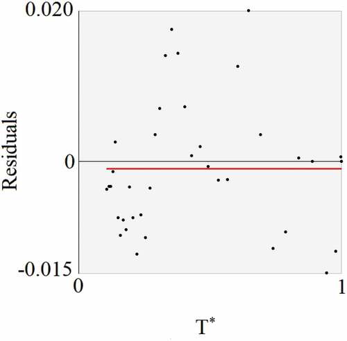
The statistical indicators chi-square and determination coefficient for the result presented in Figure 4 are χ² = 2.6981 ×10⁻³ and R² = 0.9991, respectively. The error distribution referring to the cooling kinetics is presented in Figure 5, and the residuals were calculated through the differences between experimental and simulated dimensionless temperatures, $T_i^{\ast exp}-T_i^{\ast sim}$ for all experimental points i. In Figure 5, the continuous line represents the average error, and its value was 9.48 ×10⁻⁴, in good agreement with the value zero, which is theoretically expected.

Figure 5. Error distribution. The continuous line represents the average error

Simulations for a cucumber with other dimensions

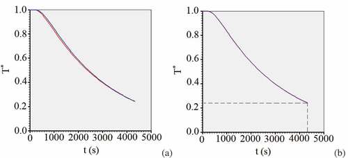
Obviously, through the results obtained in this article, it is possible to simulate cooling curves for cucumbers under similar conditions, but with other dimensions, with no need for new experiments. As an example, for a cucumber with a radius R = 0.026 m and a height L = 0.220 m, the cooling kinetics at the central point, shown in Figure 6, can be obtained by simulation. On the other hand, due to the uncertainties of the thermal properties, two lines can be drawn to obtain the confidence band of the cooling curve (Figure 6a). Due to the strong negative correlation between the thermal properties, the values α = 1.60 ×10⁻⁷ m² s⁻¹ and h = 6.10 ×10⁻⁶ m s⁻¹ were used for one simulation and α = 1.36 ×10⁻⁷ m² s⁻¹ and h = 6.60 ×10⁻⁶ m s⁻¹ were used for the other. The curve representing the simulation with average values for α and h is shown in Figure 6b.

Figure 6a shows that the confidence band is very narrow, indicating that the results obtained for α and h have a good precision to simulate the transient state of a cooling process. Figure 6b shows that, after 4320 s, the most probable value of the dimensionless temperature at the center of the second cucumber is 0.220 (about 8.0°C), while for the original cucumber a value of 0.102 (about 5.8°C) was experimentally found, as shown by Figure 4.

Discussion

In the literature, in order to simulate a transient state, many researchers determine one thermal property through empirical correlations.^[10,15] Due to that only one thermal property is determined using some optimization algorithm and an experimental dataset. In the model proposed in this article, two thermal properties (α and h) were simultaneously determined by optimization, which allowed determining the covariance between these properties. Thus, the proposed model allowed establishing a confidence band for cooling simulations of the product, using the obtained results. On the other hand, as it was observed, the proposed model included a numerical solution of the two-dimensional diffusion equation for the cylinder. Consequently, this model is useful not only to describe cylindrical product cooling, which involves a temperature variation of about 20°C or less, and therefore the thermal properties can be considered constant^{[10,11,26–28]}; but also to determine thermal properties during, for instance, the pasteurization of a product, which involves a large temperature variation and, therefore, such properties can be considered variables.^[6]

Due to the use of LS Optimizer Software, the main statistical indicators for each obtained parameter can be provided. In addition, according to Silva et al.^[3], citing Taylor^[29], the Student’s t-test is a statistical indicator that allows determining the probability $P(\bar{V}/{\sigma }_V)$ that the average value $\bar{V}$ of a parameter given in the form $V=\bar{V}\mp {\sigma }_V$ is zero, despite its value determined by optimization. In order to obtain this information for α and h using this test, the values of $P(\bar{V}/{\sigma }_V)$ were calculated, and both results were equal to zero.

Silva et al.^[8], using a one-dimensional analytical model and a technique called OREP, has obtained α = 1.47 ×10⁻⁷ m² s⁻¹ and h = 6.39 ×10⁻⁶ ms⁻¹ for the same dataset used in this article. These values are compatible with the two-dimensional numerical model proposed in the present article, which delivered the results α = (1.48 ± 0.12)×10⁻⁷ m² s⁻¹ and h = (6.35 ± 0.25)×10⁻⁶ m s⁻¹, with 95.4% confidence level. Although the two models have generated compatible results, the proposed model also provided the covariance matrix, which made it possible to determine not only the uncertainties of the thermal properties that were calculated but also the correlation between them. As mentioned before, this information is important because it allows determining a confidence band for the cooling kinetics of the product, as shown in Figure 6a. As an example, for t = 1441 s, it is possible to estimate the dimensionless temperature and also its uncertainty: T* = (0.714 ±0.008). Therefore, the percentage uncertainty of this result is 1.1%. Also, the t-test calculated for this result showed $P(\bar{V}/{\sigma }_V)$ = 0.

Figure 6. (a) Confidence band for the cooling process; (b) Cooling kinetics at the central point of a cucumber with radius R = 0.026 m and height L = 0.220 m, obtained for the average values of the thermal properties

Conclusion

The two-dimensional numerical model proposed for the cylindrical geometry in this article allowed determining simultaneously two thermal properties by optimization, their uncertainties and the correlation coefficient between them, using an experimental dataset of the cooling process of a cucumber. The results obtained for the average values of the parameters are compatible with results from the literature for the same product, and the statistical indicators chi-square and determination coefficient were χ² = 2.6981 ×10⁻³ and R² = 0.9991, respectively. Due to the covariance matrix calculated during the optimization process, it was possible to simulate a new cooling curve for a similar cucumber, but with other dimensions, including a confidence band that allowed evaluating, by graphical inspection, the precision of this new simulation.

Nomenclature

$A,B$	=	Coefficients of the discretized diffusion equation
$c_p$	=	Specific heat (J kg−1 K−1)
$h$	=	Convective heat transfer coefficient (m s−1)
$h_H$	=	Heat transfer coefficient (W m−2 K−1)
$k$	=	Thermal conductivity (W m−1 K−1)
$L$	=	Height of the cylinder (m)
$R$	=	Radius of the cylinder (m)
$R^2$	=	Determination coefficient (dimensionless)
$r$	=	Radial position (m)
$T$	=	Temperature (K)
$T_0$	=	Initial temperature (K)
$T_{\mathrm{\infty }}$	=	Cooling temperature (K)
$T_i^{exp}$	=	Experimental temperature for the point i (K)
$T_i^{sim}$	=	Simulated temperature for the point i (K)
$T_P^0$	=	Temperature in the control volume P at the beginning of a time step (K)
$T^{\ast }$	=	Dimensionless temperature
$t$	=	Cooling time (s)
$y$	=	Axial position (m)
$\mathrm{\Delta }V$	=	Volume of a control volume (m3)
$\alpha$	=	Thermal diffusivity (m2 s−1)
$\rho$	=	Density (kg m−3)
${\chi }^2$	=	Chi-square (dimensionless)

Acknowledgments

The first author would like to thank CNPq (Conselho Nacional de Desenvolvimento Científico e Tecnológico) for supporting this research study and for his research grant (Processes Number 302480/2015-3 and 444053/2014-0). On behalf of all authors, the corresponding author states that there is no conflict of interest.

Additional information

Funding

This work was supported by the Conselho Nacional de Desenvolvimento Científico e Tecnológico [302480/2015-3].

References

- Lemus-Mondaca, R. A.; Zambra, C. E.; Vega-Gálvez, A.; Moraga, N. O. Coupled 3D Heat and Mass Transfer Model for Numerical Analysis of Drying Process in Papaya Slices. J. Food Eng. 2013, 116(1), 109–117. DOI: 10.1016/j.jfoodeng.2012.10.050.
- Perussello, C. A.; Kumar, C.; de Castilhos, F.; Karim, M. A. Heat and Mass Transfer Modeling of the Osmo-Convective Drying of Yacon Roots (Smallanthus Sonchifolius). Appl. Therm. Eng. 2013, 63(1), 23–32. DOI: 10.1016/j.applthermaleng.2013.10.020.
- Silva, W. P.; Silva, C. M. D. P. S.; Gama, F. J. A. Estimation of Thermo-Physical Properties of Products with Cylindrical Shape during Drying: The Coupling between Mass and Heat. J. Food Eng. 2014, 141(1), 65–73. DOI: 10.1016/j.jfoodeng.2014.05.010.
- Bhuvaneswari, E.; Anandharamakrishnan, C. Heat Transfer Analysis of Pasteurization of Bottled Beer in a Tunnel Pasteurizer Using Computational Fluid Dynamics. Innovative Food Sci. Emerg. 2014, 23, 156–163. DOI: 10.1016/j.ifset.2014.03.004.
- Ohshima, T.; Tanino, T.; Kameda, T.; Harashima, H. Engineering of Operation Condition in Milk Pasteurization with PEF Treatment. Food Control. 2016, 68(1), 297–302. DOI: 10.1016/j.foodcont.2016.03.047.
- Silva, W. P.; Ataíde, J. S. P.; Oliveira, M. E. G.; Silva, C. M. D. P. S.; Nunes, J. S. Heat Transfer during Pasteurization of Fruit Pulps Stored in Containers with Arbitrary Geometries Obtained through Revolution of Flat Areas. J. Food Eng. 2018, 217, 58–67. DOI: 10.1016/j.jfoodeng.2017.08.012.
- Dincer, I. Determination of Thermal Diffusivities of Cylindrical Bodies Being Cooled. Int. Commun. Heat Mass Transfer. 1996, 23(5), 713–720. DOI: 10.1016/0735-1933(96)00054-1.
- Silva, W. P.; Silva, C. M. D. P. S.; Gama, F. J. A. An Improved Technique for Determining Transport Parameters in Cooling Processes. J. Food Eng. 2012, 111, 394–402. DOI: 10.1016/j.jfoodeng.2012.02.003.
- Da Silva, W. P.; Silva, C. M. D. P. S. Calculation of the Convective Heat Transfer Coefficient and Thermal Diffusivity of Cucumbers Using Numerical Simulation and the Inverse Method. J. Food Sci. Technol. 2014, 51(9), 1750–1761. DOI: 10.1007/s13197-012-0738-4.
- Erdogdu, F.; Linke, M.; Praeger, U.; Geyer, M.; Schlüter, O. Experimental Determination of Thermal Conductivity and Thermal Diffusivity of Whole Green (Unripe) and Yellow (Ripe) Cavendish Bananas under Cooling Conditions. J. Food Eng. 2014, 128, 46–52. DOI: 10.1016/j.jfoodeng.2013.12.010.
- Da Silva, W. P.; Silva, C. M. D. P. S.; Souto, L. M.; Moreira, I. S.; Silva, E. C. O. Mathematical Model for Determining Thermal Properties of Whole Bananas with Peel during the Cooling Process. J. Food Eng. 2018, 227, 11–17. DOI: 10.1016/j.jfoodeng.2018.02.003.
- Mariani, V. C.; Amarante, A. C. C.; Coelho, L. S. Estimation of Apparent Thermal Conductivity of Carrot Purée during Freezing Using Inverse Problem. Int. J. Food Sci. Technol. 2009, 44, 1292–1303. DOI: 10.1111/j.1365-2621.2009.01958.x.
- Kiani, H.; Sun, D.-W. Numerical Simulation of Heat Transfer and Phase Change during Freezing of Potatoes with Different Shapes at the Presence or Absence of Ultrasound Irradiation. Heat Mass Transfer. 2018, 54(3), 885–894. DOI: 10.1007/s00231-017-2190-5.
- Le Niliot, C.; Lefèvre, F. A Parameter Estimation Approach to Solve the Inverse Problem of Point Heat Sources Identification. Int. J. Heat Mass Transfer. 2004, 47(4), 827–841. DOI: 10.1016/j.ijheatmasstransfer.2003.08.011.
- Mariani, V. C.; Lima, A. G. B.; Coelho, L. S. Apparent Thermal Diffusivity Estimation of the Banana during Drying Using Inverse Method. J. Food Eng. 2008, 85, 569–579. DOI: 10.1016/j.jfoodeng.2007.08.018.
- Ukrainczyk, N. Thermal Diffusivity Estimation Using Numerical Inverse Solution for 1D Heat Conduction. Int. J. Heat Mass Transf. 2009, 52(25–26), 5675–5681. DOI: 10.1016/j.ijheatmasstransfer.2009.07.029.
- Muramatsu, Y.; Greiby, I.; Mishra, D. K.; Dolan, K. D. Rapid Inverse Method to Measure Thermal Diffusivity of Low-Moisture Foods. J. Food Sci. 2017, 82(2), 420–428. DOI: 10.1111/1750-3841.13563.
- Levenberg, K. A Method for the Solution of Certain Problems in Least Squares. Q. Appl. Math. 1944, 2(2), 164–168. DOI: 10.1090/qam/10666.
- Marquardt, D. W. An Algorithm for Least-Squares Estimation of Nonlinear Parameters. J. Soc. Ind. Appl. Math. 1963, 11(2), 431–441. DOI: 10.1137/0111030.
- Da Silva, W. P.; Silva, C. M. D. P. S.; Silva, D. D. P. S.; Silva, C. D. P. S.; Lima, A. G. B. Determination of Approximate Functions for the Numerical Solution of an Ordinary Differential Equation (In Portuguese: Determinação de funções Aproximadas para a solução numérica de uma equação diferencial ordinária). Revista De La Faculdad De Ingeniería UCV. 2006, 21(2), 29–37.
- Patankar, S. V. Numerical Heat Transfer and Fluid Flow; Hemisphere Publishing Corporation: New York, NY, 1980.
- Press, W. H.; Teukolsky, S. A.; Vetterling, W. T.; Flannery, B. P. Numerical Recipes in Fortran 77. The Art of Scientific Computing; Cambridge University Press: New York, 1996; Vol. 1.
- ASHRAE. Handbook of Fundamentals; American Society of Heating, Refrigerating and Air Conditioning Engineers: Atlanta, 1993.
- Sweat, V. E. Thermal Properties of Foods. In Engineering Properties of Foods; Rao, M. A., Rizvi, S. S. H., Eds.; Marcel Dekker: New York, 1986; pp 49–87.
- Fasina, O. O.; Fleming, H. P. Heat Transfer Characteristics of Cucumbers during Blanching. J. Food Eng. 2001, 47(3), 203–210. DOI: 10.1016/S0260-8774(00)00117-5.
- Campanõne, L. A.; Giner, S. A.; Mascheroni, R. H. Generalized Model for the Simulation of Food Refrigeration. Development and Validation of the Predictive Numerical Method. Int. J. Refrig. 2002, 25(7), 975–984. DOI: 10.1016/S0140-7007(01)00058-5.
- Pirozzi, D. C. Z.; Amendola, M. Mathematical Model and Numerical Simulation of Strawberry Fast Cooling with Forced Air. Eng. Agr. 2005, 25(1), 222–230. DOI: 10.1590/S0100-69162005000100025.
- Amendola, M.; Dussán-Sarria, S.; Rabello, A. A. Determination of the Convective Heat Transfer Coefficient of Fig Fruits Submitted to Forced Air Precooling. Rev. Bras. Eng. Agric. Ambient. 2009, 13, 176–182. DOI: 10.1590/S1415-43662009000200011.
- Taylor, J. R. An Introduction to Error Analysis, 2nd ed.; University Science Books: California, Sausalito, 1997.