Enhancing feedforward controller tuning via instrumental variables: with application to nanopositioning

Figures & data

Figure 1. Two degree-of-freedom control configuration.

Figure 2. The update $C_{ff}^{\Delta }(q,{\theta }^{\Delta })$ is determined based on the known r(t), and measured e^j_m(t) and y^j_m(t) in task j.

Figure 3. Tuning of a feedforward controller for a motion system. Low performance in an instrumental variable framework: significant correlation between the acceleration a(t) (dashed black) and predicted error ${\widehat{e}}^{j+1}(t,{\theta }_a)$ (red) for θ_a = 0 (left). High performance in an instrumental variable framework: a(t) (dashed black) and ${\widehat{e}}^{j+1}(t,{\theta }_a)$ (green) are uncorrelated for the minimiser ${\widehat{\theta }}_a$ of the criterion V(θ_a) in (18(18) $$\begin{array}{c}\hfill V\left({\theta }_a\right)={\left|\left|\frac{1}{N}\sum _{t=1}^{N}a\left(t\right){\widehat{e}}^{j+1}(t,{\theta }_a)\right|\right|}^2,\end{array}$$(18) ) (right). (To view this figure in colour, please see the online version of the journal).

Table 1. The comparison study presented in Sections 4 and 5 of this paper shows that optimal accuracy is not achieved with the existing approaches in van der Meulen et al. (2008) and Boeren, Oomen, et al. (2015) while the proposed approach can achieve optimal accuracy upon convergence of the proposed RIV algorithm.

Method	Instrumental	Covariance matrix PIV	Optimal
	variables		accuracy
Optimal	$z_{\text{opt}}\left(t\right)={\varphi }_r^j\left(t\right)$	$P_{IV}^{\text{opt}}={\lambda }_{\epsilon }^2{\left[\bar{\mathbb{E}}{\varphi }_r^j\left(t\right){\left({\varphi }_r^j\left(t\right)\right)}^T\right]}^{-1}$	Yes
Proposed (Section 4)	$z_{\text{p},<i>}\left(t\right)={\widehat{\varphi }}_r^j\left(t\right)$	$P_{IV,p}={\lambda }_{\epsilon }^2{\left[\bar{\mathbb{E}}{\widehat{\varphi }}_r^j\left(t\right){\left({\varphi }_r^j\left(t\right)\right)}^T\right]}^{-1}\times$	Yes
		$\left[\bar{\mathbb{E}}{\widehat{\varphi }}_r^j\left(t\right){\left({\widehat{\varphi }}_r^j\left(t\right)\right)}^T\right]{\left[\bar{\mathbb{E}}{\widehat{\varphi }}_r^j\left(t\right){\left({\varphi }_r^j\left(t\right)\right)}^T\right]}^{-T}$
Method 1 (Section 5.1)	z1(t) = Ψ(q)r(t)	$P_{IV,1}={\lambda }_{\epsilon }^2{\left[\bar{\mathbb{E}}\Psi r\left(t\right){\left({\varphi }_r^j\left(t\right)\right)}^T\right]}^{-1}\times$	No, arbitrary
		$\left[\bar{\mathbb{E}}\Psi r\left(t\right){\left(\Psi r\left(t\right)\right)}^T\right]{\left[\bar{\mathbb{E}}\Psi r\left(t\right){\left({\varphi }_r^j\left(t\right)\right)}^T\right]}^{-T}$
Method 2 (Section 5.2)	z2(t) = ϕ2(t)	$P_{IV,2}={\lambda }_{\epsilon }^2{\left[\bar{\mathbb{E}}{\varphi }_r\left(t\right){\left({\varphi }_r^j\left(t\right)\right)}^T\right]}^{-1}\times$	No, $\sqrt{2}$
		$\left[\bar{\mathbb{E}}{\varphi }_2\left(t\right){\varphi }_2^T\left(t\right)\right]{\left[\bar{\mathbb{E}}{\varphi }_r\left(t\right){\left({\varphi }_r^j\left(t\right)\right)}^T\right]}^{-T}$

Figure 4. Bode diagram of the system P.

Figure 5. Schematic illustration of a two-mass spring damper system.

Figure 6. Simulation results. Parameters $\widehat{\theta }$ as a function of tasks for m = 200 realisations for z₁(t) (left), z₂(t) (middle) and the proposed z_{p, <i >}(t) (right) show that the standard deviation of ${\widehat{\theta }}_a$ is comparable for all approaches, while the standard deviation of ${\widehat{\theta }}_s$ is significantly smaller for the proposed z_{p, <i >}(t) compared to z₁(t) and z₂(t).

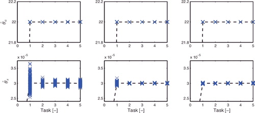
Table 2. Summary of results of Monte Carlo simulation. The mean value of ${\bar{\theta }}_a^1$ and ${\bar{\theta }}_s^1$ in task j = 1 for z_{p, <i >}(t), z₁(t) and z₂(t) confirm that unbiased parameter estimates are obtained for all methods, while the standard deviation of ${\bar{\theta }}_a^1$ and ${\bar{\theta }}_s^1$ confirms that an enhanced accuracy is obtained with the proposed approach z_{p, <i >}(t) compared to z₁(t) and z₂(t).

Method	Instrumental	Mean ${\bar{\theta }}_a^1$	Std. deviation ${\bar{\theta }}_a^1$	Mean ${\bar{\theta }}_s^1$	Std. deviation ${\bar{\theta }}_a^1$
	variables
Proposed (Section 4)	$z_{\text{p},<i>}\left(t\right)={\widehat{\varphi }}_r^j\left(t\right)$	22	2.2 × 10^−4	3 × 10^−5	1.2 × 10^−7
Method 1 (Section 5.1)	z1(t) = Ψ(q)r(t)	22	4.5 × 10^−4	3 × 10^−5	2.2 × 10^−6
Method 2 (Section 5.2)	z2(t) = ϕ2(t)	22	5.2 × 10^−4	3 × 10^−5	4.1 × 10^−7

Figure 7. Simulation results. The error signal $e_{\mathrm{ wc }}^1(t,{\widehat{\theta }}_{\mathrm{ wc }}^1)$ in task j = 1 shows that $e_{\text{wc}}^1(t,{\widehat{\theta }}_{\mathrm{ wc }}^1)$ contains a significant reference-induced component $e_r^1(t,{\widehat{\theta }}_{\mathrm{ wc }}^1)$ for z₁(t) (left), while $e_{\text{wc}}^1(t,{\widehat{\theta }}_{\mathrm{ wc }}^1)$ is dominated by e¹_w(t) for z_{p, <i >}(t) (right). For comparison, the peak value of the error signal with feedback only is given by 1 × 10⁻⁴ (m).

Figure 8. Simulation results. Cumulative power spectrum of $e_m^1(t,{\bar{\theta }}^1)$ in task j = 1 for $C_{ff}^1(q,{\bar{\theta }}^1)$ (black), and $e_{\text{wc}}^1(t,{\widehat{\theta }}_{\mathrm{ wc }}^1)$ corresponding to $C_{ff}^1(q,{\widehat{\theta }}_{\text{wc}}^1)$ for z₁(t) (red) , z₂(t) (blue) and z_{p, <i >}(t) (green). (To view this figure in colour, please see the online version of the journal.)

Figure 9. Experimental setup with $.5pt-.9pt1$ measurement system, $.5pt-.9pt2$ positioning stage, $.5pt-.9pt3$ linear magnetic actuation system and $.5pt-.9pt4$ vibration isolation table.

Figure 10. Frequency response function of the considered system P(q) in x-direction.

Figure 11. Bode diagram of the feedback controller C_fb(q) for the x-direction of the experimental setup.

Figure 12. Position r(t), velocity v(t), jerk j(t), and snap s(t) of the servo task.

Figure 13. Experimental results. The measured error signal e^j_m(t) in task j = 1 (red), j = 2 (blue) and j = 3 (green) shows that the peak value of the error signal for feedback only in task j = 1 is 4.5 × 10⁻⁶ (m), and is reduced by 97 % by using iterative feedforward control in j = 3. (To view this figure in colour, please see the online version of this journal.)

Figure 14. Experimental results. Cumulative power spectrum of the measured e^j_m(t) in task j = 1 (red), j = 2 (blue) and j = 3 (green). (To view this figure in colour, please see the online version of this journal.)

Figure 15. The two-norm of the measured error e^j_m(t) as a function of tasks shows convergence in two tasks.

Figure 16. Iterative refinement of the instruments z_{p, ** < i >}(t) after task j = 1: (C_fb + C¹_{ff, <3 >})^{− 1} (green) corresponding to the i = 3 computational iteration of Algorithm 4.1 is an improved approximation of the frequency response function of the process sensitivity S(q)P(q) (black) compared to (C_fb + C¹_{ff, <1 >})^{− 1} (dashed red) in the i = 1 iteration of Algorithm 4.1. (To view this figure in colour, please see the online version of this journal.)

Figure 17. Reference trajectory r₁ for task j = 1, 2, …, 5 (blue) and reference trajectory r₂ for task j = 6, 7, …, 10 (dashed green). (To view this figure in colour, please see the online version of this journal.)

Figure 18. Flexibility with respect to changes in the reference trajectory between tasks for ILC. Before task j = 6, the reference trajectory is changed from r₁ to r₂ (see Figure 17). For standard ILC, the measured error signal e₅(t) (blue) in task j = 5 is significantly smaller than for e₆(t) (green) in task j = 6. This confirms that for standard ILC, the servo performance is severely deteriorated if the reference is changed at j = 6. (To view this this figure in colour, please see the online version of this journal.)

Figure 19. Flexibility with respect to changes in the reference trajectory between tasks for the proposed approach in Section 4. Before task j = 6, the reference trajectory is changed from r₁ to r₂ (see Figure 17). The measured error signal e₅(t) (blue) in task j = 5 is similar to e₆(t) (green) in task j = 6, which shows that the servo performance for the proposed IV-approach is invariant to changes in the reference. (To view this figure in colour, please see the online version of this journal.)

van der Meulen, S., Tousain, R., & Bosgra, O. (2008). Fixed structure feedforward controller design exploiting iterative trials: Application to a wafer stage and a desktop printer. Journal of Dynamic Systems, Measurement, and Control, 130, 0510061–05100616.

 Web of Science ®Google Scholar

Boeren, F., Oomen, T., & Steinbuch, M. (2015). Iterative motion feedforward tuning: A data-driven approach based on instrumental variable identification. Control Engineering Practice, 37, 11–19.

 Web of Science ®Google Scholar