Trajectory-following and off-tracking minimisation of long combination vehicles: a comparison between nonlinear and linear model predictive control

Figures & data

Figure 1. Single-track representation of an A-double. The figure illustrates the vehicle dimensions, i.e. the axle positions $x_{\mathrm{a}ij}$, units front coupling positions $x_{\mathrm{c}i1}$, and units rear coupling positions $x_{\mathrm{c}i2}$ relative to the units COGs, where, i and j are unit and axle indices, respectively. Moreover, the figure shows the articulation angles ${\theta }_i$ between unit i and i + 1, steering angles ${\delta }_{ij}$, units masses $m_i$, units moments of inertia $J_i$ and the examples of the forces acting on the vehicle, i.e. the axles longitudinal forces from the propulsion/braking actuation $F_{\mathrm{xw}ij}$, the lateral forces $F_{\mathrm{yw}ij}$, air resistance $F_{\mathrm{air}}$, rolling resistance forces $F_{\mathrm{wRR}ij}$ and the gravitational forces caused by road banking $F_{\mathrm{g}i}$.

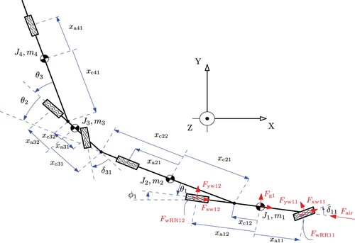
Figure 2. A single-lane-change manoeuvrer. Comparison of the different vehicle states (at COG) obtained by the two different solution methods: the nonlinear method (given by the last Newton iteration) and linear method (given by the first Newton iteration). The lower right plot shows the convergence of the linear solution to the nonlinear solution by performing Newton iterations in terms of the RMS of the velocity difference ($\frac{\mathrm{m}}{\mathrm{s}}$) between the two successive Newton iterations. The IGRTL comprises the states of a vehicle that drives straight with zero steering, braking and propulsion inputs.

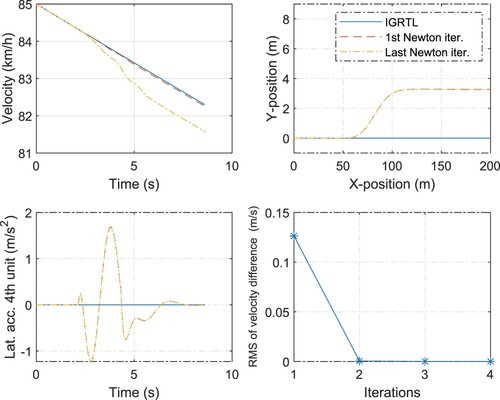
Figure 3. A U-turn manoeuvrer. Comparison of the different vehicle states (at COG) obtained by the two different solution methods: the nonlinear method (given by the last Newton iteration) and linear method (given by the first Newton iteration). The lower right plot shows the convergence of the linear solution to the nonlinear solution in terms of the RMS of the velocity difference ($\frac{\mathrm{m}}{\mathrm{s}}$) between the two successive Newton iterations. The IGRTL comprises the states of a vehicle that drives straight. The propulsion input $F_{\mathrm{xw}12=20}$ kN is the same for all the cases.

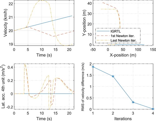
Figure 4. A single-lane-change manoeuvrer. Comparison of the different vehicle states (at COG) obtained by the two different solution methods: the nonlinear method (given by the last Newton iteration) and linear method (given by the first Newton iteration). The IGRTL comprises the states of a vehicle that drives in a sample (or guessed) single-lane-change manoeuvrer with no braking and propulsion. The reference vehicle used for generating IGRTL and the vehicle simulated by performing Newton iterations have the same steering inputs but different velocities.

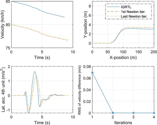
Figure 5. A U-turn manoeuvrer. Comparison of the different vehicle states (at COG) obtained by the two different solution methods: the nonlinear method (given by the last Newton iteration) and linear method (given by the first Newton iteration). The IGRTL comprises the states of a vehicle that drives in a sample (or guessed) U-turn manoeuvrer. The steering and propulsion inputs are the same in the reference vehicle used for generating IGRTL and in the vehicle simulated by performing Newton iterations, but they have different velocities.

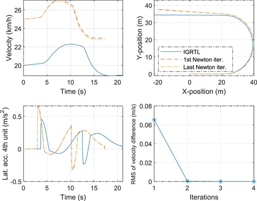
Figure 6. A single-lane-change manoeuvrer. Comparison of the different vehicle states (at COG) obtained by the two different solution methods: the nonlinear method (given by the last Newton iteration) and linear method (given by the first Newton iteration). The IGRTL comprises the states of a vehicle that drives in a sample (or guessed) single-lane-change manoeuvrer with no braking and propulsion. The reference vehicle used for generating IGRTL and the vehicle simulated by performing Newton iterations have the same steering inputs. However, the vehicle was simulated by performing Newton iterations brakes in some axles.

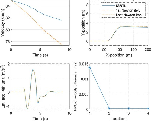
Figure 7. A U-turn manoeuvrer. Comparison of the different vehicle states (at COG) obtained by the two different solution methods: the nonlinear method (given by the last Newton iteration) and linear method (given by the first Newton iteration). The IGRTL comprises the states of a vehicle that drives in a sample (or guessed) U-turn manoeuvrer. The steering and propulsion inputs of the reference vehicle used for generating IGRTL and the vehicle simulated by performing Newton iterations are the same, but they have different velocities. However, the vehicle simulated by performing Newton iterations brakes in some axles.

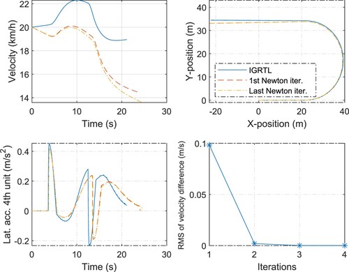
Figure 8. A single-lane-change manoeuvrer. The optimal control of the tractor front axle steering ${\delta }_{11}$ and the dolly front axle steering ${\delta }_{31}$ for following the desired trajectory and off-tracking minimisation of all the units obtained using the LTI-MPC and NMPC (SQP) solution methods. All the other inputs are kept constant, i.e. $F_{\mathrm{xw}12}=9$ kN, and the other input forces are zero. ‘Des’ refers to the desired path. All the linearisation state-input trajectories of the IGRTL are zero except for the longitudinal velocity. The NMPC (SQP) converged within two iterations. The solutions of the LTI-MPC are different from that of the NMPC (SQP). The non-optimal (non-opt) paths are obtained by simulating the LCV using a sine-steering input of the first axle ${\delta }_{11}$ similar to that obtained by the NMPC, where no optimal control of the other inputs is performed.

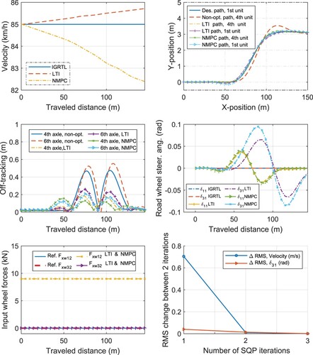
Figure 9. A single-lane-change manoeuvrer. The optimal control of the tractor front axle steering ${\delta }_{11}$ and the dolly front axle steering ${\delta }_{31}$ for following the desired path and off-tracking minimisation of all the units obtained using the LTV-MPC and NMPC (SQP) solution methods. All the other inputs are kept constant, i.e. $F_{\mathrm{xw}12}=F_{\mathrm{xw}12,\mathrm{Ref}}$ and $F_{\mathrm{xw}32}=F_{\mathrm{xw}32,\mathrm{Ref}}$, and the other input forces are zero. ‘Des’ refers to the desired path. The NMPC (SQP) is warm-started with nonzero IGRTL, e.g. a sine steering of ${\delta }_{11,\mathrm{Ref}}$. The NMPC (SQP) converged within a single iteration. The solutions of the LTV-MPC are relatively similar to that of the NMPC (SQP). The non-optimal (non-opt) paths are obtained by simulating the LCV using a sine-steering input of the first axle ${\delta }_{11}$ similar to that obtained by the NMPC, where no optimal control of the other inputs is performed.

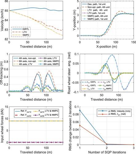
Figure 10. A U-turn manoeuvrer. The optimal control of the tractor front axle steering ${\delta }_{11}$, the dolly front axle steering ${\delta }_{31}$, and propulsion $F_{\mathrm{xw}12}$ and $F_{\mathrm{xw}32}$, whereas the other inputs are kept zero, for desired trajectory-following and off-tracking minimisation of all the units by using the LTV-MPC and NMPC (SQP) solution methods. The second axle of the dolly is equipped with an electric motor. The non-optimal (non-opt) paths are obtained by simulating the LCV using a sine-steering input of the first axle ${\delta }_{11}$ similar to that obtained by the NMPC, where no optimal control of the other inputs is performed.

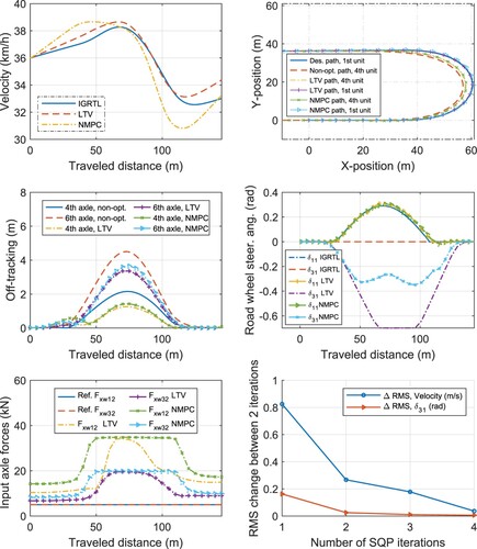
Figure 11. A-double negotiating the U-turn while the dolly steers outward.

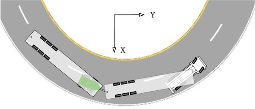
Figure 12. Lateral acceleration of the forth vehicle unit COG of the A-double during high-speed single-lane-change manoeuvrer.

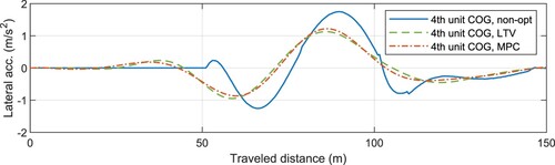
Table A1. Vehicle unit and axle parameters.

Parameter	Unit 1	Unit 2	Unit 3	Unit 4
m (kg)	10,250	22,000	3700	24,300
J (kg m${}^2$)	$0.4671\times {10}^5$	$1.6291\times {10}^5$	$0.0708\times {10}^5$	$3.0895\times {10}^5$
$x_{\mathrm{a}}$ (m)	[1.4992, −2.5858]	[−2.5687, 0]	[0.5499, −1.4501]	[−2.4778, 0]
$x_c$ (m)	[0, −2.2008]	[5.1313, −5.3187]	[3.8999, −0.4001]	[5.4222, 0]
$n_{\mathrm{ta}}$${}^{\ast }$	[2, 8]	[6, 0]	[2, 2]	[6, 0]
μ	[1, 1]	[1, 0]	[1, 1]	[1, 0]

Note: The first vehicle unit has two axles and the other units have a single axle. ‘0’ means that either the quantity is not relevant or the axle does not exist.

${}^{\ast }$ $n_{\mathrm{ta}}$ denotes the number of tires per axle.

Table A2. List of abbreviations.

Abbreviation	Meaning	Abbreviation	Meaning
COG	Centre of gravity	NMPC	Nonlinear model predictive control
DAE	Differential algebraic equation	ODE	Ordinary differential equation
IGRTL	Initial guess of the reference trajectories used for linearisation	QP	Quadratic programme
LCV	Long combination vehicle	RMS	Root mean square
LTI	Linear time-invariant	RTIs	Real-time iterations
LTV-MPC	Linear time-varying model predictive control	SQP	Sequential quadratic programming
MPC	Model predictive control	STL	Single-track linear