What is fair? Proxy discrimination vs. demographic disparities in insurance pricing

Figures & data

Figure 1. (lhs) Conditional Gaussian densities $f(x|d)$ for $d\in \mathfrak{D}=\{0,1\}$; (middle) conditional probability $\mathbb{P}(D=0|X=x)$ as a function of $x\in \mathbb{R}$; (rhs) densities of claims Y for age X = 40 and genders D = 0, 1.

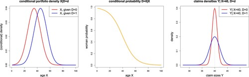
Figure 2. Best-estimate, unawareness and discrimination-free insurance prices in Example 2.14.

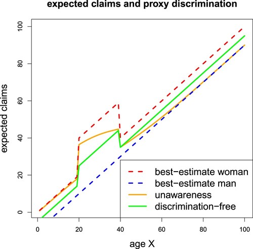
Figure 3. Average excess premium for women D = 0 compared to men D = 1, in Example 2.14, as a function of $\mathrm{Cor}(X,D)$. The dashed vertical line corresponds to the baseline scenario of $x_0=35,x_1=45$, $\mathrm{Cor}(X,D)=0.447$.

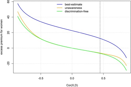
Table 1. MSEs and average prediction of the different prices in Example 2.14.

price Π	MSE	average price
Best-estimate price $\mu (\mathit{X},\mathit{D})$	100.00	41.25
Unawareness price $\mu (\mathit{X})$	197.20	41.25
DFIP ${\mu }^{\ast }(\mathit{X})$ with ${\mathbb{P}}^{\ast }(D=0)=0.50$	217.66	39.63

Figure 4. Example 2.14, revisited: conditional densities $f_d(x)=f(x|D=d)$, for $d\in \{0,1\}$, and two different choices for $f_{+}(x)$, $x\in \mathbb{R}$; for a formal definition we refer to (31(31) $F_{+}(x)=\frac{1}{2}\mathrm{\Phi }\left(\frac{x-x_0}{\tau }\right)+\frac{1}{2}\mathrm{\Phi }\left(\frac{x-x_1}{\tau }\right),$(31) )–(32(32) $F_{+}(x)=\frac{1}{2}\mathrm{\Phi }\left(\frac{x-(x_0+x_1)/2}{\tau }\right).$(32) ).

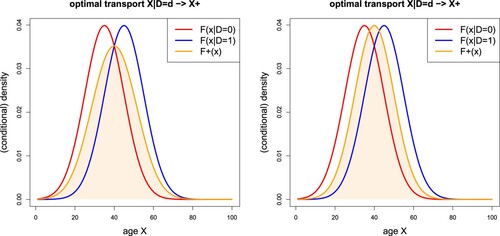
Table 2. Wasserstein distances ${\mathcal{W}}_2(F_d,F_{+})$ for the two examples (31(31) $F_{+}(x)=\frac{1}{2}\mathrm{\Phi }\left(\frac{x-x_0}{\tau }\right)+\frac{1}{2}\mathrm{\Phi }\left(\frac{x-x_1}{\tau }\right),$(31) )–(32(32) $F_{+}(x)=\frac{1}{2}\mathrm{\Phi }\left(\frac{x-(x_0+x_1)/2}{\tau }\right).$(32) ) for $F_{+}$.

	D = 0	D = 1
Input OT example (31(31) $F_{+}(x)=\frac{1}{2}\mathrm{\Phi }\left(\frac{x-x_0}{\tau }\right)+\frac{1}{2}\mathrm{\Phi }\left(\frac{x-x_1}{\tau }\right),$(31) ) for $F_{+}$	5.14	5.14
Input OT example (32(32) $F_{+}(x)=\frac{1}{2}\mathrm{\Phi }\left(\frac{x-(x_0+x_1)/2}{\tau }\right).$(32) ) for $F_{+}$	5.00	5.00

Figure 5. OT maps $T_d$ for examples (31(31) $F_{+}(x)=\frac{1}{2}\mathrm{\Phi }\left(\frac{x-x_0}{\tau }\right)+\frac{1}{2}\mathrm{\Phi }\left(\frac{x-x_1}{\tau }\right),$(31) )–(32(32) $F_{+}(x)=\frac{1}{2}\mathrm{\Phi }\left(\frac{x-(x_0+x_1)/2}{\tau }\right).$(32) ) of $F_{+}$ with the original age X on the x-axis and the transformed ages $X_{+}=T_d(X)$ on the y-axis; the black dotted line is the 45${}^{\mathrm{o}}$ diagonal.

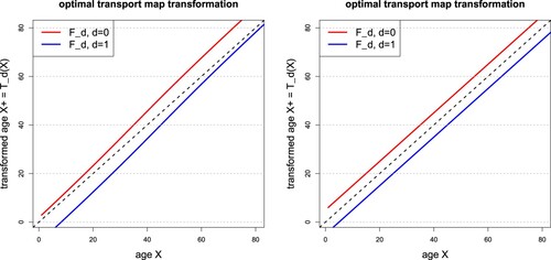
Figure 6. OT input transformed model prices $\hat{\mu }({\mathit{X}}_{+})$ for examples (31(31) $F_{+}(x)=\frac{1}{2}\mathrm{\Phi }\left(\frac{x-x_0}{\tau }\right)+\frac{1}{2}\mathrm{\Phi }\left(\frac{x-x_1}{\tau }\right),$(31) )–(32(32) $F_{+}(x)=\frac{1}{2}\mathrm{\Phi }\left(\frac{x-(x_0+x_1)/2}{\tau }\right).$(32) ) of $F_{+}$.

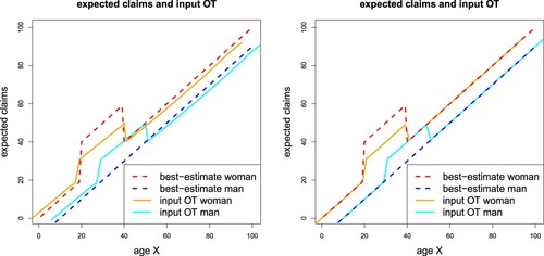
Table 3. MSEs and average prediction of the different prices in Example 2.14.

Average price	MSE	Average price
Best-estimate price $\mu (\mathit{X},\mathit{D})$	100.00	41.25
Unawareness price $\mu (\mathit{X})$	197.20	41.25
Input OT map of (31(31) $F_{+}(x)=\frac{1}{2}\mathrm{\Phi }\left(\frac{x-x_0}{\tau }\right)+\frac{1}{2}\mathrm{\Phi }\left(\frac{x-x_1}{\tau }\right),$(31) ) for $\hat{\mu }({\mathit{X}}_{+})$	162.77	41.25
Input OT map of (32(32) $F_{+}(x)=\frac{1}{2}\mathrm{\Phi }\left(\frac{x-(x_0+x_1)/2}{\tau }\right).$(32) ) for $\hat{\mu }({\mathit{X}}_{+})$	162.72	41.25
Input OT map of (32(32) $F_{+}(x)=\frac{1}{2}\mathrm{\Phi }\left(\frac{x-(x_0+x_1)/2}{\tau }\right).$(32) ) for best-estimate $\hat{\mu }({\mathit{X}}_{+},\mathit{D})$	100.60	41.24

Figure 7. Changed age profiles with $x_0=45$ (women) and $x_1=35$ (men): (lhs) conditional probability $\mathbb{P}(D=0|X=x)$ as a function of $x\in \mathbb{R}$; (middle) best-estimate, unawareness and discrimination-free insurance prices; (rhs) OT input transformed model prices $\hat{\mu }({\mathit{X}}_{+})$ for example (32(32) $F_{+}(x)=\frac{1}{2}\mathrm{\Phi }\left(\frac{x-(x_0+x_1)/2}{\tau }\right).$(32) ) of $F_{+}$.

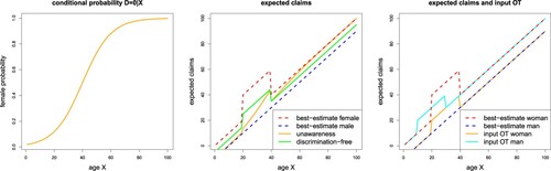
Table 4. Changed role of ages of women and men, setting $x_0=45$ and $x_1=35$.

price Π	MSE	average price
Best-estimate price $\mu (\mathit{X},\mathit{D})$	100.00	38.01
Unawareness price $\mu (\mathit{X})$	197.12	38.01
Input OT map of (31(31) $F_{+}(x)=\frac{1}{2}\mathrm{\Phi }\left(\frac{x-x_0}{\tau }\right)+\frac{1}{2}\mathrm{\Phi }\left(\frac{x-x_1}{\tau }\right),$(31) ) for $\hat{\mu }({\mathit{X}}_{+})$	290.68	38.01
Input OT map of (32(32) $F_{+}(x)=\frac{1}{2}\mathrm{\Phi }\left(\frac{x-(x_0+x_1)/2}{\tau }\right).$(32) ) for $\hat{\mu }({\mathit{X}}_{+})$	290.64	38.01

Figure 8. OT output post-processing density $g_{+}$ and distribution $G_{+}$.

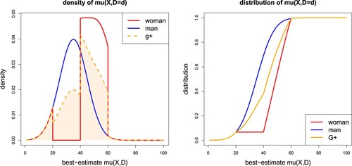
Figure 9. (Top) OT output post-processed prices ${\mu }_{+}={\mu }_{+}(\mathit{x};\mathit{d})$ expressed in their original features $\mathit{x}$ and separated by gender $\mathit{d}$, see (38(38) $(\mathit{x},\mathit{d})\mapsto {\mu }_{+}={\mu }_{+}(\mathit{x};\mathit{d})=G_{+}^{-1}\circ G_{\mathit{d}}(\mu (\mathit{x},\mathit{d}))\in \mathbb{R}.$(38) ); (bottom-lhs) OT input pre-processing taken from Figure 6; (bottom-rhs) unawareness price and DFIP taken from Figure 2.

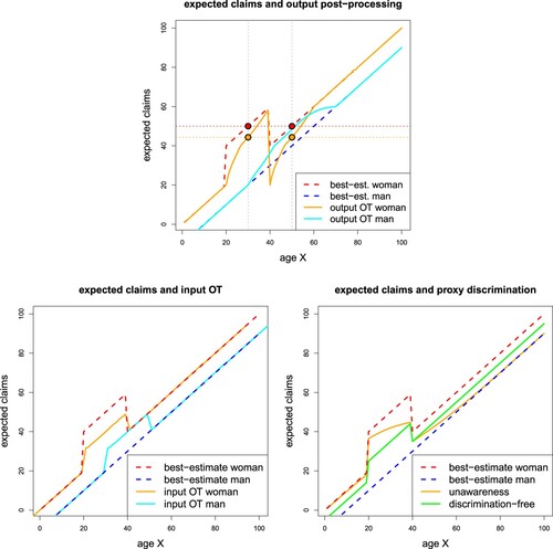
Table 5. MSEs and average prediction of the different prices in Example 2.14.

price Π	MSE	average price
Best-estimate price $\mu (\mathit{X},\mathit{D})$	100.00	41.25
Unawareness price $\mu (\mathit{X})$	197.20	41.25
Output OT map of (39(39) $g_{+}(m)=\frac{1}{2}(g_0(m)+g_1(m))\mathrm{for}m\in \mathbb{R}.$(39) ) for ${\mu }_{+}$	152.97	41.25

Table

Addressing proxy discrimination	Addressing fairness
Model post-processing of prices $\mu (\mathit{X},\mathit{D})$	Input pre-processing of features $\mathit{X}$
Change of probability from $\mathbb{P}$ to ${\mathbb{P}}^{\ast }$	Deformation of $\mathit{X}$ to ${\mathit{X}}_{+}$
Independence of $\mathit{X}$ and $\mathit{D}$ under ${\mathbb{P}}^{\ast }$	Independence of ${\mathit{X}}_{+}$ and $\mathit{D}$ under $\mathbb{P}$
Dependence of $\mathit{X}$ and $\mathit{D}$ under $\mathbb{P}$ ···	Dependence of $\mathit{X}$ and $\mathit{D}$ under $\mathbb{P}$ ···
···  does not matter for price adjustments	···  matters for price adjustments