Stability of vitamin C in broccoli based on the chemical reaction kinetics, micro-region state diagram, and empirical correlations

Figures & data

Figure 1. A typical graph of DMTA frequency sweep of freeze-dried broccoli powder at 0.25% compression

Figure 2. Storage and loss modulus of freeze-dried broccoli powder as a function of DMTA temperature ramp (frequency: 0.1 Hz, temperature: −30°C to 150°C and heating rate: 5°C/min)

Table 1. Rate constant for vitamin C degradation as a function of temperature and moisture content

Fresh Broccoli Xw: 0.9 g/g sample (Tm′)u: −30.0°C and (Tg′′′)u: 32.2°C			Freeze-dried Broccoli Xw: 0.067 Tgo: −0.8°C Xb: 0.083 g/g sample at 20°C
T (°C)	k (s^−1)	r^2	T (°C)	k (s^−1)	r^2
−80	1.110 × 10^−8	0.598	−80	1.748 × 10^−9	0.699
−60	1.276 × 10^−8	0.817	−60	-
−40	4.410 × 10^−8	0.781	−40	2.567 × 10^−9	0.537
−20	8.301 × 10^−8	0.907	−20	1.735 × 10^−8	0.892
5	5.030 × 10^−7	0.894	5	1.193 × 10^−8	0.902
20	4.030 × 10^−6	0.993	20	6.976 × 10^−8	0.939
45	3.210 × 10^−5	0.947	45	6.022 × 10^−7	0.891
60	1.230 × 10^−4	0.914	60	1.765 × 10^−6	0.840
70	4.900 × 10^−4	0.876	70	5.381 × 10^−6	0.839
80	2.970 × 10^−4	0.896	80	7.429 × 10^−6	0.855
110	4.580 × 10^−4	0.971	110	8.233 × 10^−5	0.952
120	5.650 × 10^−3	0.971	120	1.021 × 10^−4	0.890

Notes: Data of fresh broccoli at 5–120°C were adopted from Al-Habsi et al. (2019). Data source of (T_m′)_u, (T_g′′′)_u, X_w: Moisture content (g/g sample), X_b: BET-monolayer (Suresh et al. 2017).

Figure 3. Typical graphs showing (a) The change in vitamin C concentration over time in Freeze-dried sample stored at −80°C, (b) Plot of ln (C/C_o) versus time for freeze-dried sample stored at −80°C, (c) The change in vitamin C concentration over time in fresh sample stored at 60°C, and (d): Plot of ln (C/C_o) versus time for fresh sample

Table 2. The activation energy of the three temperature regions

Phase	Fresh Broccoli		Freeze-dried Broccoli
	Xw: 0.90 g/g sample		Xw: 0.067 g/g sample
	Pre-exponent factor	Ea (kJ/mole)	Pre-exponent factor	Ea (kJ/mole)
Phase 1	4.831 × 10^−5	13.6 (−80°C to −20°C)	4.985 × 10^−6	13.1 (−80°C to 5°C)
Phase 2	7.286 × 10^7	75.0 (−20°C to 60°C)	1.548 × 10^5	69.6 (5°C to 70°C)
Phase 3	1.242 × 10^3	43.6 (60°C to 120°C)	4.817 × 10^5	72.4 (70°C to 120°C)

Figure 4. (a) Plot of log k as a function of temperature for the fresh sample, (b) Arrhenius plot for the fresh sample, (c) Plot of log k as a function of temperature for the freeze-dried sample, (d) Arrhenius plot for the freeze-dried sample

Figure 5. State diagram of broccoli (abc: freezing curve, egf glass transition line, irh: BET-monolayer, kj: solids melting-decomposition line, u: T_m′, experimental ultimate maximal-freeze-concentration melting temperature, v: T_g′′′, experimental ultimate maximal-freeze-concentration glass transition temperature, b: X_s′, conceptual maximal-freeze-concentration solids, d: T_g′, conceptual maximal-freeze-concentration glass transition temperature, m: X_s′′′, conceptual maximal-freeze-concentration solids, g: T_g′′, hypothetical maximal-freeze-concentration glass transition temperature, and 1–13: indicates the micro-regions 1–13)

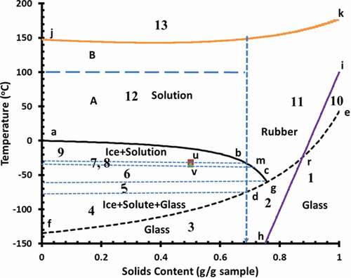
Figure 6. Bi-plot of the PCA showing different cluster of micro-regions

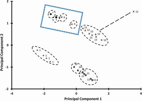
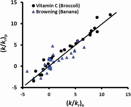
Figure 7. (k/k_r)_p predicted from Equations 3(3) $lnk=-\left(\frac{E_a}{R}\right)\left(\frac{1}{T}\right)+b$(3) and 4(4) $lnk=-33.42+0.0123\left(\frac{X_w}{X_b}\right)+15.96\left(\frac{T}{T_x}\right)$(4) as a function of (k/k_r)_e and best prediction line