Airborne LiDAR point cloud in mapping of fluvial forms: a case study of a Hungarian floodplain

Figures & data

Figure 1. Location of the study area. For full colour versions of the figures in this paper, please see the online version.

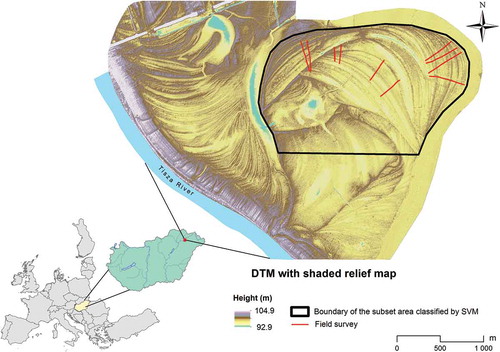
Figure 2. Sampling of the point cloud to analyze the interspersion of the classified points.

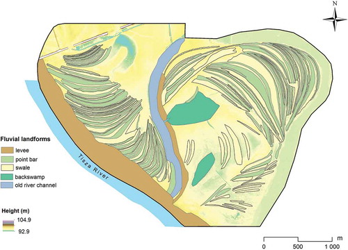
Figure 3. The visually interpreted fluvial landforms.

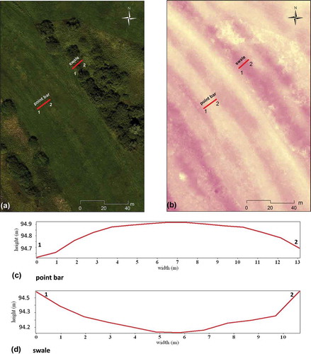
Figure 4. The main steps of our workflow.

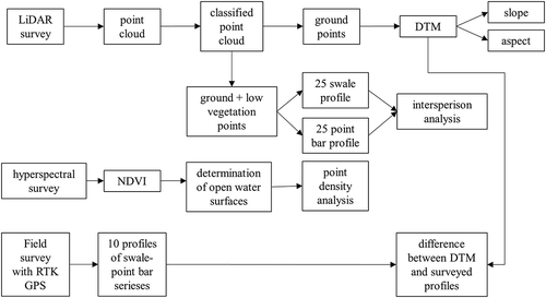
Table 1. The average number of points in the cross-section cuboids by floodplain forms (mean ± standard deviation; n: varying width to ensure 30 points/n point density).

Width of cross-section cuboids (m)	Swales	Point bars
4	20.8 ± 12.1	20.9 ± 8.7
6	31.4 ± 18.2	31.3 ± 12.2
8	41.6 ± 23.8	41.2 ± 16.1
10	52.2 ± 30.4	51.1 ± 20.4
n	30	30

Table 2. Characteristics of the point cloud in the study area and by landforms.

	Study area		Point bars		Swales
	Number of points	Points/m^2	Number of points	Points/m^2	Number of points	Points/m^2
Points	93,839,032	9.94	16,179,966	9.82	16,705,014	9.51
Ground points	46,901,456	4.96	9,676,940	5.88	8,629,469	4.91
Missing ground points in a m^2 (%)		11.5		6.8		10.2
Low vegetation points (0–0.5 m)	14,232,174	1.50	2787,820	1.69	3407,885	1.94
Medium vegetation points (0.51–1.50 m)	12,072,124	1.28	1121,205	0.68	2046,105	1.16
High vegetation points (1.51 m)	20,618,516	2.18	2591,643	1.57	2617,142	1.49
Noise	7018	0.00	943	0.00	2111	0.00
Nonclassified	7744	0.00	1415	0.00	2302	0.00

Figure 5. The shape of a characteristic point bar and swale [(a) orthophoto, (b) DTM, (c) profile of the point bar, and (d) profile of the swale).

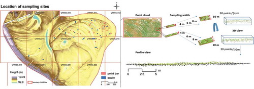
Table 3. Comparison of swales and point bars by the applied landscape variables (mean ± standard deviation).

Landscape variable	Point bar	Swale	Mean difference	Sig.	Effect size (r)
DTM (m, a.s.l.)	94.7 ± 0.2	94.5 ± 0.2	0.15	0.003	0.36
Aspect (degree, azimuth)	167 ± 87	174 ± 90	5.80	0.334	0.09
Slope (percent)	0.05 ± 0.03	0.05 ± 0.03	0.002	0.440	0.12
NDVI	0.34 ± 0.09	0.34 ± 0.09	0.008	0.641	0.05

Figure 6. Height differences between the DTM and field survey by floodplain forms and vegetation types (a), and their interaction plot by floodplain forms (b), and by vegetation types (c) (legend: P: point bar; S: swale; CL: clear areas with short grass, R: reed and sedge, DR: dense reed and sedge; W: woods, HS: short (mowed) grass with haystocks).

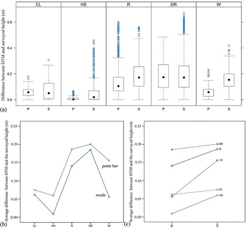
Figure 7. Interspersion of ground and vegetation points according to AI (a) and CONTAG (b) indices and the mixture of the classified point clouds of swales and point bars (c).

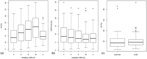
Table 4. Error matrix of the landscape variables.

Variables involved in the classification	OA (%)	Point bar	Swale
		PA (%)
DTM	66	79	54
Aspect	52	23	82
Slope	54	38	69
NDVI	44	14	90
DTM + NDVI	69	73	65
DTM + aspect	68	75	60
DTM + slope	68	74	63
DTM + NDVI + slope	71	73	67
DTM + NDVI + aspect	69	72	67
DTM + aspect + slope	68	73	62
NDVI + aspect + slope	59	50	67
NDVI + aspect + slope + DTM	71	74	70

OA: overall accuracy; PA: producer’s accuracy.

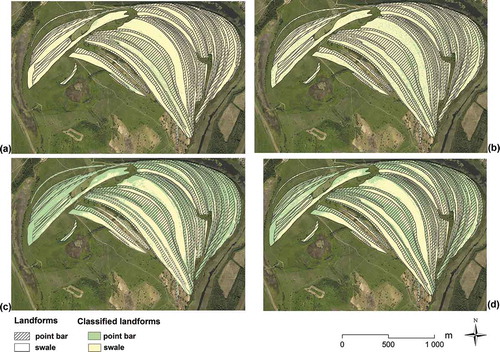
Figure 8. Maps resulting from SVM classification [(a) NDVI; (b) slope; (c) DTM; (d) DTM + slope + aspect + NDVI).