Regional-scale burned area mapping in Mediterranean regions based on the multitemporal composite integration of Sentinel-1 and Sentinel-2 data

Figures & data

Figure 1. Location of the burned study area in Europe (top-left), in Portugal (bottom-left). The image on the right shows the overview of the study area (Sentinel-2 composite image based on the second-lowest NIR criterion, false-color composite SWIR-NIR-RED); the red areas represent the burned surfaces.

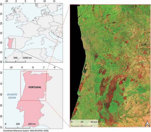
Table 1. Sentinel-2 (S2) and Sentinel-1 (S1) image mosaic dates used in this study (format: year/month/day), acquired before and during the fire season.

Time of acquisition	Sentinel-2 Multispectral Level-2A	Sentinel-1 IW mode Level-1 GRDH
Pre-Fire	2017/04/15	2017/04/14
	2017/04/25	2017/04/20
	2017/04/28	2017/05/02
	2017/05/08	2017/05/14
	2017/05/25	2017/05/26
Fire season	2017/06/04	2017/06/07
	2017/06/07	2017/06/25
	2017/06/24	2017/07/07
	2017/07/07	2017/07/19
	2017/07/14	2017/07/25
	2017/07/24	2017/08/06
	2017/08/03	2017/08/18
	2017/08/13	2017/08/24
	2017/08/23	2017/09/05
	2017/09/02	2017/09/17
	2017/09/12	2017/09/23
	2017/09/22	2017/10/05
	2017/10/02	2017/10/17
	2017/10/22	2017/10/23
	2017/10/26	2017/10/29

Figure 2. The flowchart illustrates the second-lowest NIR (secMinNIR) scheme, SAR criteria, and their placement within the workflow.

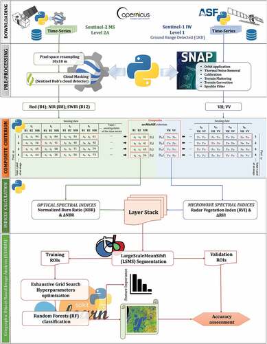
Table 2. Parameter values of the random forest (RF) classifier tested through an exhaustive grid search approach to set the optimal combination.

Parameter name	Values set	Description
n_estimators	100, 650, 1200, 1750, 2300, 2850, 3400, 3950, 4500, 5050, 5600, 6150, 6700, 7250, 7800, 8350, 8900, 9450, 10,000	The number of trees in the RF model
max_depth	10, 20, 30, 40, 50, 60, 70, 80, 90, 100, 110, 300, 500, 800, 1000	The maximum depth of the tree
min_samples_split	2, 5, 10	The minimum number of samples required to split an internal node
min_samples_leaf	1, 2, 4	The minimum number of samples required to be at a leaf node
max_features	“auto,” “None,” “log2”	The number of features to consider when looking for the best split

Figure 3. Multitemporal composite output relative to the optical part of the dataset (Sentinel-2) that resulted from processing fire season images (June-October). Five illustrative areas are shown on a more detailed scale beside the overview of the entire study area (top left). The images are shown in RGB combination (R = B12; G = B8; B = B4).

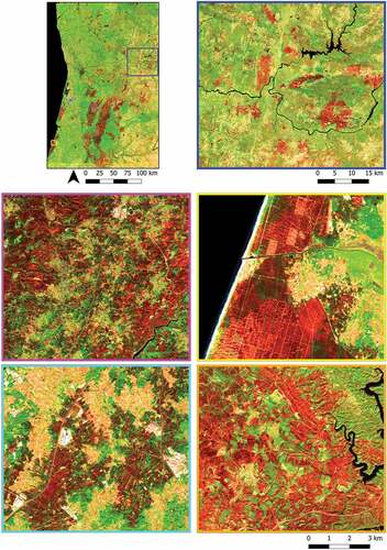
Figure 4. The Figure shows the ΔNBR index map calculated by applying the subtraction NBR_post-fire – NBR_pre-fire. The darker areas correspond to lower index values, while the brighter pixel means represent higher values. The overview of the entire study area is shown on the top-left; five illustrative areas are shown on a more detailed scale.

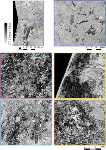
Figure 5. The ΔRVI index map, calculated by applying the subtraction RVI_post-fire – RVI_pre-fire. The darker areas correspond to lower index values, while the brighter pixels represent higher values. The overview of the entire study area is shown on the top-left; five illustrative areas are shown on a more detailed scale.

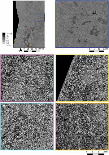
Figure 6. Segmentation output that resulted from applying the Large-Scale-Mean-Shift (LSMS) algorithm to the S1+ S2 dataset. The segments are presented in a blue border, while the base map is the S2 composite image based on the second-lowest NIR (SecMinNIR) criterion (false-color composite B12-B8-B4). The segmentation is shown for the entire study area (top left) and five detailed illustrative areas.

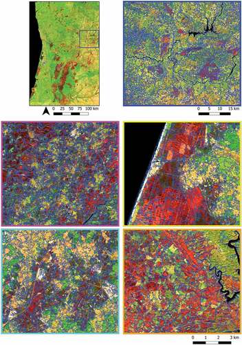
Figure 7. Segmentation output that resulted from applying the Large-Scale-Mean-Shift (LSMS) algorithm to the S2 dataset. The segments are presented in a blue border, while the base map is the S2 composite image based on the second-lowest NIR (SecMinNIR) criterion (false color composite B12-B8-B4). The segmentation is shown for the entire study area (top left) and five detailed illustrative areas.

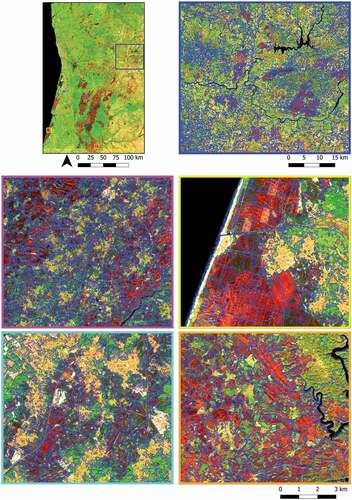
Table 3. The final combination of Random Forest (RF) parameter values that resulted from the exhaustive grid search-based test and was used in the classification approach for both datasets (S1+ S2 and S2).

Parameter name	Values (S1+ S2)	Values (S2)
n_estimators	1200	1750
max_depth	110	65
min_samples_split	2	2
min_samples_leaf	1	1
max_features	“auto”	“auto”

Figure 8. Classification output, based on the S1+ S2 dataset. Segments showing only the burned class (blue) are overlaid on an S2 composite image based on the second-lowest NIR (SecMinNIR) criterion (false color composite B12-B8-B4). The classification is shown for the entire study area (top left) and five detailed illustrative areas.

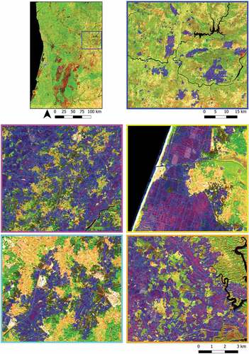
Figure 9. Classification output, based on the S2 dataset. Segments showing only the burned class (blue) are overlaid on an S2 composite image based on the second-lowest NIR (SecMinNIR) criterion (false color composite B12-B8-B4). The classification is shown for the entire study area (top left) and five detailed illustrative areas.

Figure 10. Feature importance for burned area mapping (Gini importance), expressed by each spectral feature (mean and variance) used in the classification process for both dataset combinations: S1+ S2 and S2.

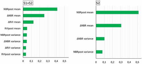
Table 4. Weighted descriptive statistics (average, µ_sw; standard deviation, σ_sw), computed using the values of the spectral features (mean, m_s; variance, v_s) of all the classified polygons of each S1+ S2 input layer (ΔNBR, NBR, ΔRVI, RVI), separately for burned and unburned classes.

Image layer	Spectral features	Weighted average (µsw)		Weighted standard deviation (σsw)
		Burned	Unburned	Burned	Unburned
ΔNBR	ms	29.7601	45.8026	4.8992	3.8137
	vs	2.4165	1.4901	2.8745	2.1497
NBR	ms	12.3907	23.8265	2.8068	4.1501
	v^2	1.1457	1.5632	1.9540	1.8859
ΔRVI	ms	47.4288	49.5496	1.7230	1.0755
	v^2	0.8201	0.7188	1.5703	1.5541
RVI	ms	17.5369	20.3481	3.8364	3.9241
	vs	2.6855	3.2240	5.6704	4.2363

Data availability statement

The data supporting this study’s findings are available from the corresponding author upon reasonable request. These data were derived from the following resources available in the public domain: ESA Sentinel Homepage (2021).