Obtaining orange juice–maltodextrin powders without structure collapse based on the glass transition temperature and degree of polymerization

Figures & data

Figure 1. Digital images of the powders obtained after the spray drying process: (a) OJ–M_c, (b) OJ–M₁₀, (c) OJ–M₂₀, (d) OJ–M₄₀ and (e) OJ.

Figura 1. Imágenes digitales de los polvos obtenidos después del proceso de secado por aspersión: A) OJ-M_c, b) OJ-M₁₀, c) OJ-M₂₀, d) OJ-M₄₀ y e) OJ.

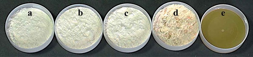
Figure 2. Diffractograms determined by XRD of the powders: (a) OJ–M_c, (b) OJ–M₁₀ and (c) OJ–M₂₀. The corresponding water activity (a_w) is indicated by the number written next to each curve: (1) 0.07, (2) 0.328, (3) 0.434, (4) 0.528 and (5) 0.718.

Figura 2. Difractogramas obtenidos por XRD de los polvos: A) OJ-M_c, b) OJ-M₁₀, y c) OJ-M₂₀. La actividad de agua (a_w) correspondiente se indica en cada curva con la siguiente numeración: 1) 0,07, 2) 0,328, 3) 0,434, 4) 0,528 y 5) 0,718.

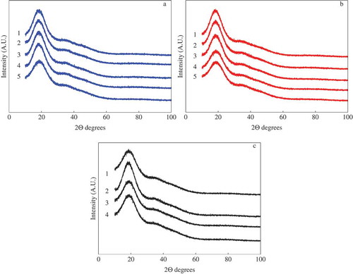
Figure 3. Thermograms determined by MDSC of the powders: (a) OJ-M_c, (b) OJ–M₁₀ and (c) OJ–M₂₀. Each plot contains three curves, identified in the following order as: total heat flow (on top), reversible heat flow (in the middle) and non-reversible heat flow (bottom curve).

Figura 3. Termogramas obtenidos por MDSC de los polvos: A) OJ-M_c, b) OJ-M₁₀, y c) OJ-M₂₀. Cada gráfica contiene tres curvas, que se identifican en el siguiente orden: flujo de calor total (curva superior), flujo de calor reversible (curva media) y flujo de calor no reversible (curva inferior).

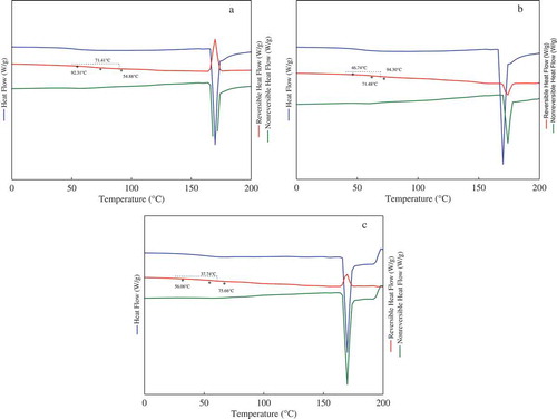
Table 1. T_g values of the OJ–MX systems at the different water activities determined by MDSC.

Table 1. Valores de T_g de los sistemas de OJ-MX´s a diferentes actividades de agua determinados por MDSC.

aw	OJ–MC	Mc^a	OJ–M10	M10^a	OJ–M20	M20^a
0.07	71.5 ± 0.8	100.2 ± 2.8	71.2 ± 0.40	90.4 ± 2.8	56.1 ± 0.49	80.0 ± 2.2
0.328	58.1 ± 0.9	74.0 ± 0.2	54.2 ± 0.60	80.2 ± 0.9	43.3 ± 0.49	50.6 ± 1.0
0.434	23.5 ± 0.3	69.4 ± 2.1	33.1 ± 0.20	50.5 ± 3.0	30.1 ± 1.00	48.3 ± 0.9
0.528	11.7 ± 0.5	43.0 ± 0.6	20.8 ± 0.81	47.9 ± 0.5	22.2 ± 0.80	40.9 ± 1.8
0.718	−06.0 ± 0.1	38.8 ± 2.5	12.0 ± 1.17	40.6 ± 0.7	−12.1 ± 0.50	10.5 ± 4.0
0.75	−13.2 ± 0.3	20.2 ± 0.7	−22.5 ± 0.83	20.9 ± 0.2	−32.0 ± 0.67	00.9 ± 0.7

^a T_g data obtained from Saavedra et al. (2015) for the individual maltodextrins.

^aValores de T_g para las diferentes maltodextrinas obtenidos por Saavedra et al. (2015).

Table 2. Comparison of the T_gS values calculated with Gordon–Taylor equation and the T_g values determined by MDSC of the OJ–MX systems at the different water activities.

Table 2. Comparación de los valores de T_gS calculados mediante la ecuación de Gordon-Taylor y los valores de T_g determinados mediante MDSC de los sistemas de OJ-MX´s a diferentes actividades de agua.

aw	OJ–Mc	ΔOJ–Mc	OJ–M10	ΔOJ–M10	OJ–M20	ΔOJ–M20
0.07	66.63	4.86	64.01	7.18	54.61	1.48
0.328	39.28	15.78	48.41	15.31	30.09	0.006
0.434	24.65	12.95	21.48	0.682	21.62	0.57
0.528	2.12	8.12	12.32	0.32	19.16	31.26
0.718	−28.79	15.59	−15.24	7.25	−29.95	2.04
0.75	−33.8	5.90	−29.90	4.00	−40.12	1.92

Δ corresponds to the difference between the T_g data determined experimentally and calculated employing Equation (4).

Δ corresponde a la diferencia entre el valor de T_g determinado experimentalmente y el valor calculado empleando la Ecuación (4).

Table 3. The k_w and k_M values of Gordon–Taylor equation of the OJ–MX systems.

Table 3. Valores de los parámetros k_w y k_M de la ecuación de Gordon-Taylor de los sistemas de OJ-MX´s.

System	kW	kM	R
OJ–MC	0.168	1.799	0.948
OJ–M10	0.623	10.363	0.979
OJ–M20	3318	54971	0.938
Overall	0.218	2.93	0.938

Saavedra, L.Z., Leyva, P.C., Araujo, D.S.B., Toxqui, T.A., & Borrás, E.A.J. (2015). Technological application of maltodextrins according to the degree of polymerization. Molecules, 20, 21067–21081. doi:10.3390/molecules201219746

 PubMed Web of Science ®Google Scholar