Synergistic strengthening of crack-free Al–Zn–Mg–Cu alloys with hierarchical microstructures achieved via laser powder bed fusion

Figures & data

Figure 1. (a) EBSD inverse pole figure map of the as-built alloy. (b1) BSE image of the boundary between CG and EG regions. High-magnification BSE image of (b2) CG and (b3) EG regions. TEM-EDS results for (c) CG and (d) EG regions. SAED patterns in (c) and (d) correspond to the diffraction patterns of θ-Al₂Cu and L1₂-Al₃Zr, respectively. (e) Schematic of grain morphology and distribution of precipitates in the Al–Zn–Mg–Cu–Zr alloy. (f) Hardness measurement results at each region in as-built Al–Zn–Mg–Cu–Zr alloy.

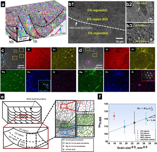
Figure 2. Tensile test results of as-built Al–Zn–Mg–Cu–Zr alloy and other as-built Al alloys with inoculants [18,24,32].

Figure 3. (a) Micro digital image correlation results. (a1), (a2), and (a3) Local equivalent strain (ε_e) maps at the initial state and the global strains of 2% and 4%, respectively. (b) Line profile of ε_e from A₀ to A₂₀ along the white line in Figure 3(a3). (c) and (d) GNDs density maps of the initial state and at the global strains of 4%, respectively. (e) Schematic of the accumulation of GNDs at the interfaces.

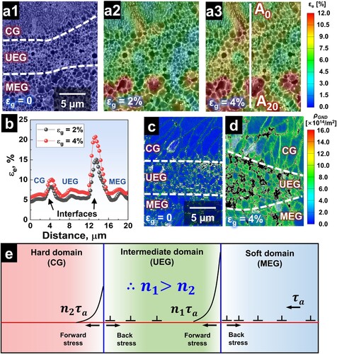
Table 1. Average equivalent strains in each domain.

εg	εe in CG	εe in UEG	εe in MEG
2%	5.04 ± 0.24%	5.42 ± 0.32%	5.80 ± 0.67%
4%	6.14 ± 0.22%	6.86 ± 0.49%	7.00 ± 0.35%

Figure 4. Tensile test results for as-built Al–Zn–Mg–Cu–Zr alloy. (a) True strain–stress curve of the LUR test. (b) HDI stress and effective stress of Al–Zn–Mg–Cu–Zr and Al–Mg–Sc–Zr [18]. alloys, respectively. (c) YSs of Al–Mg–Sc–Zr [18] and Al–Zn–Mg–Cu–Zr alloys. (d) Ashby plot of as-built Al–Zn–Mg–Cu–Zr, Al–Zn–Mg–Cu–Sc–Zr [7], Al–Cu–Mg–Zr [24,38,39], Al–Mg–Sc–Zr [18,40], and Al–Mg–Zr alloys [32].

Wang Z, Lin X, Kang N, et al. Laser powder bed fusion of high-strength Sc/Zr-modified Al–Mg alloy: phase selection, microstructural/mechanical heterogeneity, and tensile deformation behavior. J Mater Sci Technol. 2021;95:40–56. doi:10.1016/j.jmst.2021.03.069

 Web of Science ®Google Scholar

Wang Y, Lin X, Kang N, et al. Laser powder bed fusion of Zr-modified Al-Cu-Mg alloy: Crack-inhibiting, grain refinement, and mechanical properties. Mater Sci Eng, A. 2022;838:142618. doi:10.1016/j.msea.2022.142618

 Web of Science ®Google Scholar

Xu R, Li R, Yuan T, et al. Laser powder bed fusion of Al–Mg–Zr alloy: Microstructure, mechanical properties and dynamic precipitation. Mater Sci Eng, A. 2022;859:144181. doi:10.1016/j.msea.2022.144181

 Web of Science ®Google Scholar

Zhu Z, Ng FL, Seet HL, et al. Superior mechanical properties of a selective-laser-melted AlZnMgCuScZr alloy enabled by a tunable hierarchical microstructure and dual-nanoprecipitation. Mater Today. 2022;52:90–101. doi:10.1016/j.mattod.2021.11.019

 Web of Science ®Google Scholar

Wang J, Zhang S, Lu R, et al. A crack-free and high-strength Al-Cu-Mg-Mn-Zr alloy fabricated by laser powder bed fusion. Mater Sci Eng A. 2022;854:143731. doi:10.1016/j.msea.2022.143731

 Web of Science ®Google Scholar

Wang Y, Lin X, Zhao Y, et al. Microstructure and strengthening mechanisms of Zr-modified Al–Cu–Mg alloy processed by selective laser melting. Mater Sci Eng A. 2023;870:144874. doi:10.1016/j.msea.2023.144874

 Web of Science ®Google Scholar

Li X, Liu Y, Zhou Z. Grain refinement and performance enhancement of laser powder bed fusion in-situ processed Al-Mg alloy modified by ScH3 and ZrH2. Mater Charact. 2022;190:112068. doi:10.1016/j.matchar.2022.112068

 Web of Science ®Google Scholar