Enhancing feedforward controller tuning via instrumental variables: with application to nanopositioning

ABSTRACT

Feedforward control enables high performance of a motion system. Recently, algorithms have been proposed that eliminate bias errors in tuning the parameters of a feedforward controller. The aim of this paper is to develop a new algorithm that combines unbiased parameter estimates with optimal accuracy in terms of variance. A simulation study is presented to illustrate the poor accuracy properties of pre-existing algorithms compared to the proposed approach. Experimental results obtained on an industrial nanopositioning system confirm the practical relevance of the proposed method.

KEYWORDS:

• Feedforward control
• system identification
• data-driven control
• precision motion systems

1. Introduction

Challenging requirements on positioning accuracy often necessitate the use of feedforward control for motion systems, since feedforward can effectively compensate for the error induced by known, repeating disturbances. Examples include atomic force microscopes (Butterworth, Pao, & Abramovitch, 2012; Clayton, Tien, Leang, Zou, & Devasia, 2009; Kara-Mohamed, Heath, & Lanzon, 2015), robotics (Khalil & Dombre, 2002, Chapter 14) and wafer scanners (Mishra, Coaplen, & Tomizuka, 2007; Oomen et al., 2014; van der Meulen, Tousain, & Bosgra, 2008). Traditional approaches that can potentially achieve these requirements on positioning accuracy include iterative learning control (ILC) (Bristow, Tharayil, & Alleyne, 2006; Gorinevsky, 2002) and model-based feedforward (Butterworth et al., 2012; Zhong, Pao, & de Callafon, 2012).

ILC algorithms update the feedforward signal by learning from previous tasks under the assumption that the task is repetitive. ILC consequently enables superior performance with respect to model-based feedforward for a specific task by compensating for all repetitive disturbances. However, changes in the reference signal typically result in significant performance deterioration (see, e.g. Hoelzle, Johnson, & Alleyne, 2014). Motion systems are typically confronted with similar yet slightly different reference signals (Lambrechts, Boerlage, & Steinbuch, 2005; Oomen et al., 2014). In contrast to ILC, model-based feedforward results in moderate performance for a class of reference signals instead of only one specific reference (Butterworth et al., 2012). Note that the performance for model-based feedforward is highly dependent on the model quality of the parametric model of the system and the accuracy of model-inversion (Devasia, 2002).

By introducing basis functions in ILC, the advantages of model-based feedforward and ILC are combined in van de Wijdeven and Bosgra (2010). This approach is further improved in van der Meulen et al. (2008), where the need for an approximate model of the system, as is common in ILC, is eliminated by exploiting results from iterative feedback tuning (Bazanella, Campestrini, & Eckhard, 2012). The iterative feedforward control approach in van der Meulen et al. (2008) is extended to multivariable systems and input shaping in Heertjes, Hennekens, and Steinbuch (2010) and Boeren, Bruijnen, van Dijk, and Oomen (2014), respectively. However, in Boeren, Oomen, and Steinbuch (2015), it is shown that the least-squares algorithm used in van der Meulen et al. (2008) can lead to a bias error in the estimated parameters. A new algorithm is proposed in Boeren, Oomen, et al. (2015) based on instrumental variable (IV) techniques that results in unbiased parameter estimates. However, accuracy in terms of variance of the estimate has not yet been investigated.

Although iterative feedforward control based on instrumental variables is promising for motion control, existing approaches suffer from poor accuracy properties in terms of variance. This severely limits the practical applicability of existing approaches in case of noisy signals. This paper aims to reveal non-optimal accuracy for the approaches in Boeren, Oomen, et al. (2015) and van der Meulen et al. (2008), and develop an algorithm that leads to optimal accuracy in the presence of noise.

The contributions of this paper are fourfold. First, an analysis is provided to show that the approaches in Boeren, Oomen, et al. (2015) and van der Meulen et al. (2008) lead to poor accuracy in terms of variance. Therefore, variance results developed in open-loop identification (Söderström & Stoica, 1983, Chapters 5 and 6) and closed-loop identification (Forssell, 1999; Gilson & Van den Hof, 2005) are extended towards iterative feedforward control. As a second contribution, this insight in the accuracy aspects is exploited to develop an algorithm that achieves optimal accuracy. The proposed algorithm (1) exploits an iterative refined instrumental variable (RIV) method that is similar to the approaches presented in Young (1976, 2015), Young and Jakeman (1979), Jakeman and Young (1979), and Young and Jakeman (1980), and (2) is closely connected to the estimation of inverse systems (see, e.g. Jung & Enqvist, 2013). Third, a simulation study is presented to (1) illustrate that the proposed algorithm leads to enhanced accuracy properties compared to pre-existing approaches and (2) confirm the significance of the accuracy of parameter estimates on the achievable performance. As a final contribution, experimental results confirm the practical relevance of the proposed algorithm. This paper significantly extends earlier results reported in Boeren, Bruijnen, and Oomen (2014) and Boeren, Oomen, and Steinbuch (2014) by thorough proofs and extended experimental results. Related data-driven tuning algorithms are available in Formentin, van Heusden, and Karimi (2013b), Karimi, Butcher, and Longchamp (2008), and Kim and Zou (2013). Furthermore, instrumental variable approaches are often used for estimating the parameters of industrial robots (see, e.g. Janot, Vandanjon, & Gautier, 2014a, 2014b; Puthenpura & Sinha, 1986; Yoshida, Ikeda, & Mayeda, 1992).

This paper is organised as follows. In Section 2, the problem formulation is outlined. In Section 3, asymptotic expressions for optimal accuracy are developed for feedforward control. To provide a concise presentation of the contributions of this paper, the second contribution is presented before the first contribution is explained. That is, a new tuning algorithm for iterative feedforward control is proposed in Section 4. Then, in Section 5, the accuracy properties of existing approaches are analysed. In Section 6, a simulation study of a motion system is presented to compare the proposed and pre-existing approaches. In Section 7, the theoretical results are confirmed by experiments on an industrial nanopositioning system. Finally, conclusions are drawn in Section 8.

Notation:

The variable q denotes the forward shift operator qu(t) = u(t + 1). For a vector x, ||x||²_W = x^TWx. A positive-definite matrix A is denoted as A ≻ 0. Also, A − B ≻ 0 is denoted as A ≻ B. A positive-semidefinite matrix A is denoted as A ⪰ 0. Let $\mathbb{R}\left[q\right]$ denotes the real polynomials in q. Also, $\mathbb{E}\left(x\right)={\int }_{-\infty }^{\infty }xf\left(x\right)dx,$ with probability density function f (x), $\bar{\mathbb{E}}\left(x\right)={lim}_{N\to \infty }\frac{1}{N}{\sum }_{t=1}^N\mathbb{E}\left(x\right),$ where N is the number of samples.

2. Problem definition

2.1 Problem setup

Consider the two degree-of-freedom control configuration as depicted in Figure 1. The true unknown system P(q) is assumed to be discrete-time, single-input single-output, and linear time-invariant, with rational representation $$\begin{array}{c}\hfill P\left(q\right)={\displaystyle \frac{B_0\left(q\right)}{A_0\left(q\right)}},\end{array}$$ where $B_0\left(q\right),A_0\left(q\right)\in \mathbb{R}\left[q\right]$. The control configuration consists of a given stabilising feedback controller C_fb(q), and a feedforward controller C^j_ff(q). The index j denotes the jth task in a sequence of finite time tasks of length N samples, where j = 0, 1, ..., M. Furthermore, T_s denotes the sampling time.

Figure 1. Two degree-of-freedom control configuration.

Let r denote the reference signal. Typically, r is designed as a known nth-order multi-segment polynomial trajectory with constraints on the first n derivatives, as in, e.g. Biagiotti and Melchiorri (2012) and Lambrechts et al. (2005). Also, w^j(t) = H(q)ε^j(t) denotes an unknown disturbance, where H(q) is a monic, asymptotically stable, proper system, and {ε^j(t)} is normally distributed white noise with zero mean and variance λ²_ϵ. Hence, w^j and r are uncorrelated. The feedforward signal is denoted by u^j_ff, while the measured signals e^j_m and y^j_m in the jth task are given by (1) $$\begin{array}{c}\hfill \begin{array}{c}\hfill e_m^j\left(t\right)=e_r^j\left(t\right)-e_w^j\left(t\right),\\ \hfill y_m^j\left(t\right)=y_r^j\left(t\right)+y_w^j\left(t\right),\end{array}\end{array}$$(1) with (2) $$\begin{array}{c}\hfill \begin{array}{c}{e}_r^j\left(t\right)=S\left(q\right)(1-P\left(q\right)C_{ff}^j\left(q\right))r\left(t\right),\hfill \\ e_w^j=S\left(q\right)w^j\left(t\right),\hfill \\ y_r^j\left(t\right)=S\left(q\right)P\left(q\right)(C_{fb}\left(q\right)+C_{ff}^j\left(q\right))r\left(t\right),\hfill \\ y_w^j=S\left(q\right)w^j\left(t\right),\hfill \end{array}\end{array}$$(2) and sensitivity function S(q) = (1 + P(q)C_fb(q))⁻¹. Since P(q) is assumed to be unknown and w^j is an unknown disturbance, it is not possible to determine e^j_r and e^j_w (resp. y^j_r and y^j_w) based on the measured signal e^j_m (resp. y^j_m).

2.2 Iterative feedforward: batch-wise tuning

In iterative feedforward control, the measured signals e^j_m(t) and y^j_m(t), for t = 1, ..., N, are stored. Hence, the data set that is used for the estimation of the feedforward controller is given by $$\begin{array}{cc}& e_m^j=\left[e_m^j\left(1\right),e_m^j\left(2\right),\cdots ,e_m^j\left(N\right)\right],\hfill \\ & y_m^j=\left[y_m^j\left(1\right),y_m^j\left(2\right),\cdots ,y_m^j\left(N\right)\right].\hfill \end{array}$$ After the jth task is finished, this batch of measured data is used to perform an offline update of the existing feedforward controller C^j_ff(q), i.e. $$\begin{array}{c}\hfill C_{ff}^{j+1}\left(q\right)=C_{ff}^j\left(q\right)+C_{ff}^{\Delta }\left(q\right),\end{array}$$ before initiating the (j + 1)th task.

To establish the main ideas in this paper and provide a fair comparison, the feedforward controller C^{j + 1}_ff(q) is parametrised similar to Lambrechts et al. (2005), van der Meulen et al. (2008), Heertjes et al. (2010), and Boeren, Bruijnen, van Dijk, et al. (2014) as (3) $$\begin{array}{cc}\hfill C_{ff}^{j+1}(q,{\theta }^{j+1})& =C_{ff}^j(q,{\theta }^j)+C_{ff}^{\Delta }(q,{\theta }^{\Delta })\hfill \\ & =\sum _{i=1}^{n_{\theta }}{\psi }_i\left(q^{-1}\right)({\theta }_i^j+{\theta }_i^{\Delta }),\hfill \end{array}$$(3) where ${\theta }_i^{j+1}={\theta }_i^j+{\theta }_i^{\Delta }$, and ψ_i(q⁻¹) are basis functions. The update C^Δ_ff(q, θ^Δ) is given by (4) $$\begin{array}{cc}\hfill C_{ff}^{\Delta }(q,{\theta }^{\Delta })& =\sum _{i=1}^{n_{\theta }}{\psi }_i\left(q^{-1}\right){\theta }_i^{\Delta }=\Psi \left(q\right){\theta }^{\Delta },\hfill \end{array}$$(4) with parameters ${\theta }^{\Delta }={[{\theta }_1^{\Delta }{\theta }_2^{\Delta }\cdots {\theta }_{n_{\theta }}^{\Delta }]}^T\in {\mathbb{R}}^{n_{\theta }},$ and polynomial basis functions $$\begin{array}{c}\hfill \Psi \left(q\right)=[{\psi }_1\left(q^{-1}\right){\psi }_2\left(q^{-1}\right)\cdots {\psi }_{n_{\theta }}\left(q^{-1}\right)].\end{array}$$ To illustrate a typical selection of the parameter vector ${\theta }^{\Delta }$ and basis functions Ψ(q), consider the following example that is aimed at feedforward control for motion systems.

Example 2.1:

Let C^j_ff(q) = 0, i.e. only a feedback controller C_fb(q) is used in task j, and let r(t) be a fourth-order reference trajectory. A typical parametrisation of $C_{ff}^{\Delta }(q,{\theta }^{\Delta })$ is given by (5) $$\begin{array}{c}\hfill C_{ff}^{\Delta }(q,{\theta }^{\Delta })={\psi }_a\left(q^{-1}\right){\theta }_a^j+{\psi }_s\left(q^{-1}\right){\theta }_s^j,\end{array}$$(5) with basis functions $$\begin{array}{c}\hfill {\psi }_a\left(q^{-1}\right)={\left({\displaystyle \frac{1-q^{-1}}{T_s}}\right)}^2,{\psi }_s\left(q^{-1}\right)={\left({\displaystyle \frac{1-q^{-1}}{T_s}}\right)}^4,\end{array}$$ parameters θ^j = [θ^j_a, θ_s^j]^T, and sampling time T_s. The parametrisation in (5(5) $$\begin{array}{c}\hfill C_{ff}^{\Delta }(q,{\theta }^{\Delta })={\psi }_a\left(q^{-1}\right){\theta }_a^j+{\psi }_s\left(q^{-1}\right){\theta }_s^j,\end{array}$$(5) ) consists of acceleration feedforward with acceleration a(t) = ψ_a(q⁻¹)r(t), i.e., the second derivative of r(t), and snap feedforward with snap s(t) = ψ_s(q⁻¹)r(t), i.e. the fourth derivative of r(t). Furthermore, θ_a denotes the mass of the system, while θ_s denotes the snap parameter. As such, C^Δ_ff(q, θ^Δ) in (5(5) $$\begin{array}{c}\hfill C_{ff}^{\Delta }(q,{\theta }^{\Delta })={\psi }_a\left(q^{-1}\right){\theta }_a^j+{\psi }_s\left(q^{-1}\right){\theta }_s^j,\end{array}$$(5) ) can compensate for the dominant component of the reference-induced error (see, e.g. Lambrechts et al., 2005). Note that double (and fourth) differentiation is possible since r(t) is a deterministic and known signal. The corresponding feedforward signal u_ff(t) is given by $$\begin{array}{c}\hfill u_{ff}^{j+1}\left(t\right)=C_{ff}^{\Delta }(q,{\theta }^{\Delta })r\left(t\right)={\theta }_{a}a\left(t\right)+{\theta }_{s}s\left(t\right).\end{array}$$ The approach proposed in this paper aims to estimate the parameters θ_a and θ_s based on measured data.

The use of feedforward is a standard approach to obtain a small error signal e^j_m(t) when tracking a reference trajectory r(t) (see, e.g. Steinbuch & Norg, 1998). By subdividing e^j_m(t) into e^j_r(t) and e^j_w(t), as defined in (2(2) $$\begin{array}{c}\hfill \begin{array}{c}{e}_r^j\left(t\right)=S\left(q\right)(1-P\left(q\right)C_{ff}^j\left(q\right))r\left(t\right),\hfill \\ e_w^j=S\left(q\right)w^j\left(t\right),\hfill \\ y_r^j\left(t\right)=S\left(q\right)P\left(q\right)(C_{fb}\left(q\right)+C_{ff}^j\left(q\right))r\left(t\right),\hfill \\ y_w^j=S\left(q\right)w^j\left(t\right),\hfill \end{array}\end{array}$$(2) ), it is immediately clear that C^{j + 1}_ff(q, θ^{j + 1}) has no influence on e^j_w(t). Indeed, the goal of feedforward control is to determine a C^{j + 1}_ff(q, θ^{j + 1}) that minimises the reference-induced error e^{j + 1}_r(t, θ^{j + 1}) for t = 1, ..., N in a suitable sense. Given the definition of C^{j + 1}_ff(q, θ^{j + 1}) in (3(3) $$\begin{array}{cc}\hfill C_{ff}^{j+1}(q,{\theta }^{j+1})& =C_{ff}^j(q,{\theta }^j)+C_{ff}^{\Delta }(q,{\theta }^{\Delta })\hfill \\ & =\sum _{i=1}^{n_{\theta }}{\psi }_i\left(q^{-1}\right)({\theta }_i^j+{\theta }_i^{\Delta }),\hfill \end{array}$$(3) ), the aim of this paper is to determine θ^{j + 1} such that e^{j + 1}_r(t, θ^{j + 1}) is as small as possible. It directly follows from (2(2) $$\begin{array}{c}\hfill \begin{array}{c}{e}_r^j\left(t\right)=S\left(q\right)(1-P\left(q\right)C_{ff}^j\left(q\right))r\left(t\right),\hfill \\ e_w^j=S\left(q\right)w^j\left(t\right),\hfill \\ y_r^j\left(t\right)=S\left(q\right)P\left(q\right)(C_{fb}\left(q\right)+C_{ff}^j\left(q\right))r\left(t\right),\hfill \\ y_w^j=S\left(q\right)w^j\left(t\right),\hfill \end{array}\end{array}$$(2) ) that (6) $$\begin{array}{c}\hfill e_r^{j+1}(t,{\theta }^{j+1})=S\left(q\right)(1-P\left(q\right)C_{ff}^{j+1}(q,{\theta }^{j+1}))r\left(t\right),\end{array}$$(6) and e^{j + 1}_r(t, θ^{j + 1}) = 0 for all t if C^{j + 1}_ff(q, θ^{j + 1}) = P^{− 1}(q). However, since P(q) is assumed to be unknown, it is not possible to determine either P⁻¹(q), or determine e^{j + 1}_r(t, θ^{j + 1}) before initiating the (j + 1)th task. Instead, the measured signal e^j_m(t) in the jth task, contaminated by w^j(t), is used in an optimisation problem to determine C^{j + 1}_ff(q, θ^{j + 1}). That is, the aim in iterative feedforward control is to determine the parameters ${\widehat{\theta }}^{\Delta }$ in (4(4) $$\begin{array}{cc}\hfill C_{ff}^{\Delta }(q,{\theta }^{\Delta })& =\sum _{i=1}^{n_{\theta }}{\psi }_i\left(q^{-1}\right){\theta }_i^{\Delta }=\Psi \left(q\right){\theta }^{\Delta },\hfill \end{array}$$(4) ), before starting the (j + 1)th task, from the optimisation problem (7) $$\begin{array}{c}\hfill {\widehat{\theta }}^{\Delta }=arg\underset{{\theta }^{\Delta }}{min}V\left({\theta }^{\Delta }\right),\end{array}$$(7) where the criterion V(θ^Δ) is based on the stored signals e^j_m(t) and y^j_m(t) for t = 1, ..., N, as measured in the jth task. Then, C^{j + 1}_ff(q, θ^{j + 1}) is determined according to (3(3) $$\begin{array}{cc}\hfill C_{ff}^{j+1}(q,{\theta }^{j+1})& =C_{ff}^j(q,{\theta }^j)+C_{ff}^{\Delta }(q,{\theta }^{\Delta })\hfill \\ & =\sum _{i=1}^{n_{\theta }}{\psi }_i\left(q^{-1}\right)({\theta }_i^j+{\theta }_i^{\Delta }),\hfill \end{array}$$(3) ). Next, two assumptions are introduced.

Assumption 2.1:

C_fb(q) is designed such that S(q)H(q) = 1, where the noise model is parametrised as $$\begin{array}{c}\hfill H\left(q\right)=\frac{D\left(q^{-1}\right)}{C\left(q^{-1}\right)}=\frac{1+d_1{q}^{-1}+\cdots +d_m{q}^{-m}}{1+c_1{q}^{-1}+\cdots +c_m{q}^{-m}}.\end{array}$$

Assumption 2.2:

The true unknown system is given by $$\begin{array}{c}\hfill P_0=\frac{1}{A_0\left(q^{-1}\right)}=\frac{1}{1+a_1{q}^{-1}+\cdots +a_n{q}^{-n}}.\end{array}$$

Concerning Assumption 2.1, recall from (6(6) $$\begin{array}{c}\hfill e_r^{j+1}(t,{\theta }^{j+1})=S\left(q\right)(1-P\left(q\right)C_{ff}^{j+1}(q,{\theta }^{j+1}))r\left(t\right),\end{array}$$(6) ) that C^j_ff(q, θ^j) aims to minimise e^j_r(t), i.e. the error induced by the known r(t). In the optimal case, it holds that e^j_r(t) = 0 for all t. In contrast, the main goal of the feedback controller C_fb(q) is to compensate for w^j(t) in view of minimising e^j_w(t). These disturbances are assumed to be stochastic with a certain spectrum. Typically, the dominant disturbances are in the low-frequency range, e.g. due to amplifier noise (Fleming, 2014), cable slab, commutation errors, or immersion water-flow in lithographic applications. Then, C_fb(q) is designed to compensate for these disturbances, in which case the optimal result is e^j_w(t) = ϵ^j(t), i.e. the error signal being white noise. Clearly, this corresponds to S(q)H(q) = 1. Similar approximations are used in the identification of robotics (see, e.g. Janot, Gautier, Jubien, & Vandanjon (2014)). Assumption 2.1 can be achieved by, e.g. using traditional PID tuning, possibly with error-based retuning (van de Wal, van Baars, & Sperling, 2000), and common LQG control designs (Åström, 1970, Section 6.2). In a typical approach to design C_fb(q) such that S(q)H(q) = 1, e^j_m(t) is measured in an experiment where r(t) = 0 for all t. For this case, e^j_r(t) = 0 for all t, and consequently e^j_m(t) = e_w^j(t). Then, C_fb(q) is tuned until e^j_m(t) = ϵ^j(t), i.e. e^j_m(t) being white noise.

Concerning Assumption 2.2, the assumption that P(q) = 1/A₀(q) implies that there is a θ^{j + 1} such that C^{j + 1}_ff(q, θ^{j + 1}) = P^{− 1}(q). This result immediately follows by observing that P⁻¹(q) = A₀(q) and C^{j + 1}_ff(q, θ^{j + 1}) is restricted to a polynomial parametrisation as in (3(3) $$\begin{array}{cc}\hfill C_{ff}^{j+1}(q,{\theta }^{j+1})& =C_{ff}^j(q,{\theta }^j)+C_{ff}^{\Delta }(q,{\theta }^{\Delta })\hfill \\ & =\sum _{i=1}^{n_{\theta }}{\psi }_i\left(q^{-1}\right)({\theta }_i^j+{\theta }_i^{\Delta }),\hfill \end{array}$$(3) ). This assumption may appear as a stringent requirement on P(q). However, for a general class of motion systems as described in Lambrechts et al. (2005), the reference signal r(t) has a dominant low-frequency signal content, and P⁻¹(q) can be accurately described by an acceleration-dependent and snap-dependent term (Boerlage, Tousain, & Steinbuch, 2004). That is, high-frequency dynamic aspects are concealed by the specific input design of r(t) (see also Hjalmarsson (2009) for a further explanation of this aspect). These results will be corroborated by the simulation example in Section 6 and the experimental results in Section 7, where it is shown that the reference-induced contribution to the error signal can be almost completely compensated for by using C^{j + 1}_ff(q, θ^{j + 1}) as in (3(3) $$\begin{array}{cc}\hfill C_{ff}^{j+1}(q,{\theta }^{j+1})& =C_{ff}^j(q,{\theta }^j)+C_{ff}^{\Delta }(q,{\theta }^{\Delta })\hfill \\ & =\sum _{i=1}^{n_{\theta }}{\psi }_i\left(q^{-1}\right)({\theta }_i^j+{\theta }_i^{\Delta }),\hfill \end{array}$$(3) ) of low degree. The proposed approach can be extended by allowing a more general parametrisation for C^{j + 1}_ff(q, θ^{j + 1}), as in, e.g. Boeren, Blanken, Bruijnen, and Oomen (2015) and Boeren, Bruijnen, van Dijk, et al. (2014) if a reference is needed with a significant high-frequency signal content.

Throughout, measured data from a single task is used to determine ${\widehat{\theta }}^{\Delta }$ according to (7(7) $$\begin{array}{c}\hfill {\widehat{\theta }}^{\Delta }=arg\underset{{\theta }^{\Delta }}{min}V\left({\theta }^{\Delta }\right),\end{array}$$(7) ). This approach is pursued since it can effectively handle slow variations that are typically present in a motion system, for example, wear, by means of continuous adaptation of the feedforward parameters. Note that the presented approach can be directly extended to exploit data from multiple tasks (e.g. as in Gunnarsson and Norrlöf (2001, 2006) and Kushner and Yin (2003)).

3. Optimal feedforward based on instrumental variables

3.1 Iterative feedforward control

Based on the known r(t) and measured e^j_m(t) and y^j_m(t) in task j, the predicted error ${\widehat{ϵ}}^{j+1}(t,{\theta }^{\Delta })$ in task j + 1 can be determined as (see Figure 2): (8) $$\begin{array}{c}\hfill {\widehat{ϵ}}^{j+1}(t,{\theta }^{\Delta })=e_m^j\left(t\right)-S\left(q\right)P\left(q\right)C_{ff}^{\Delta }(q,{\theta }^{\Delta })r\left(t\right).\end{array}$$(8) In the proposed iterative feedforward control approach, the parameters θ^Δ should be estimated directly from measured data as is done in Hjalmarsson, Gevers, Gunnarsson, and Lequin (1998), i.e. without estimating a model of P(q). As such, (8(8) $$\begin{array}{c}\hfill {\widehat{ϵ}}^{j+1}(t,{\theta }^{\Delta })=e_m^j\left(t\right)-S\left(q\right)P\left(q\right)C_{ff}^{\Delta }(q,{\theta }^{\Delta })r\left(t\right).\end{array}$$(8) ) cannot be directly used to determine θ^Δ. Instead, the following estimate of ${\widehat{ϵ}}^{j+1}(t,{\theta }^{\Delta })$ is used (9) $$\begin{array}{c}\hfill {\widehat{e}}^{j+1}(t,{\theta }^{\Delta })=e_m^j\left(t\right)-C_{ff}^{\Delta }(q,{\theta }^{\Delta })C^{-1}{y}_m^j\left(t\right),\end{array}$$(9) where C = (C_fb(q) + C^j_ff(q)). To show that (9(9) $$\begin{array}{c}\hfill {\widehat{e}}^{j+1}(t,{\theta }^{\Delta })=e_m^j\left(t\right)-C_{ff}^{\Delta }(q,{\theta }^{\Delta })C^{-1}{y}_m^j\left(t\right),\end{array}$$(9) ) is a suitable estimate of (8(8) $$\begin{array}{c}\hfill {\widehat{ϵ}}^{j+1}(t,{\theta }^{\Delta })=e_m^j\left(t\right)-S\left(q\right)P\left(q\right)C_{ff}^{\Delta }(q,{\theta }^{\Delta })r\left(t\right).\end{array}$$(8) ), note that the commutative property of SISO systems enables rewriting y^j_m(t) in (1(1) $$\begin{array}{c}\hfill \begin{array}{c}\hfill e_m^j\left(t\right)=e_r^j\left(t\right)-e_w^j\left(t\right),\\ \hfill y_m^j\left(t\right)=y_r^j\left(t\right)+y_w^j\left(t\right),\end{array}\end{array}$$(1) ) as y^j_m(t) = (C_fb(q) + C^j_ff(q))S(q)P(q)r(t) + S(q)w^j(t). Rearranging terms leads to (10) $$\begin{array}{c}\hfill C^{-1}\left(q\right)y_m^j\left(t\right)=S\left(q\right)P\left(q\right)r\left(t\right)+C^{-1}\left(q\right)S\left(q\right)w^j\left(t\right).\end{array}$$(10) Clearly, ${\widehat{e}}^{j+1}(t,{\theta }^{\Delta })={\widehat{ϵ}}^{j+1}(t,{\theta }^{\Delta })$ if w^j(t) is equal to zero. Moreover, by taking the expectation of (10(10) $$\begin{array}{c}\hfill C^{-1}\left(q\right)y_m^j\left(t\right)=S\left(q\right)P\left(q\right)r\left(t\right)+C^{-1}\left(q\right)S\left(q\right)w^j\left(t\right).\end{array}$$(10) ), it follows that (11) $$\begin{array}{cc}\hfill \mathbb{E}\left\{C^{-1}\left(q\right)y_m^j\left(t\right)\right\}=\mathbb{E}& \{S\left(q\right)P\left(q\right)r\left(t\right)+C^{-1}\left(q\right)S\left(q\right)w^j\left(t\right)\}.\hfill \end{array}$$(11) By noting that r(t) is deterministic, it follows that $\mathbb{E}S\left(q\right)P\left(q\right)r\left(t\right)=S\left(q\right)P\left(q\right)r\left(t\right)$. Furthermore, for w^j(t) as defined in Section 2.1, it is immediately clear that $\mathbb{E}{C}^{-1}\left(q\right)S\left(q\right)w^j\left(t\right)=0$(see, e.g. Söderström, 2002, Lemma 4.1). By combining these results, (11(11) $$\begin{array}{cc}\hfill \mathbb{E}\left\{C^{-1}\left(q\right)y_m^j\left(t\right)\right\}=\mathbb{E}& \{S\left(q\right)P\left(q\right)r\left(t\right)+C^{-1}\left(q\right)S\left(q\right)w^j\left(t\right)\}.\hfill \end{array}$$(11) ) implies that (10(10) $$\begin{array}{c}\hfill C^{-1}\left(q\right)y_m^j\left(t\right)=S\left(q\right)P\left(q\right)r\left(t\right)+C^{-1}\left(q\right)S\left(q\right)w^j\left(t\right).\end{array}$$(10) ) is an unbiased estimator of S(q)P(q)r(t).

Figure 2. The update $C_{ff}^{\Delta }(q,{\theta }^{\Delta })$ is determined based on the known r(t), and measured e^j_m(t) and y^j_m(t) in task j.

In the remainder of this paper, (9(9) $$\begin{array}{c}\hfill {\widehat{e}}^{j+1}(t,{\theta }^{\Delta })=e_m^j\left(t\right)-C_{ff}^{\Delta }(q,{\theta }^{\Delta })C^{-1}{y}_m^j\left(t\right),\end{array}$$(9) ) is used as the predicted error in task j + 1. Substituting the parametrisation defined in (4(4) $$\begin{array}{cc}\hfill C_{ff}^{\Delta }(q,{\theta }^{\Delta })& =\sum _{i=1}^{n_{\theta }}{\psi }_i\left(q^{-1}\right){\theta }_i^{\Delta }=\Psi \left(q\right){\theta }^{\Delta },\hfill \end{array}$$(4) ) into (9(9) $$\begin{array}{c}\hfill {\widehat{e}}^{j+1}(t,{\theta }^{\Delta })=e_m^j\left(t\right)-C_{ff}^{\Delta }(q,{\theta }^{\Delta })C^{-1}{y}_m^j\left(t\right),\end{array}$$(9) ) and rearranging terms leads to the following estimation equation: (12) $$\begin{array}{c}\hfill {\widehat{e}}^{j+1}(t,{\theta }^{\Delta })=e_m^j\left(t\right)-{\left({\varphi }^j\left(t\right)\right)}^T{\theta }^{\Delta },\end{array}$$(12) where (13) $$\begin{array}{c}\hfill {\varphi }^j\left(t\right)=\Psi \left(q\right){(C_{fb}\left(q\right)+C_{ff}^j\left(q\right))}^{-1}{y}_m^j\left(t\right)\in {\mathbb{R}}^{n_{\theta }}.\end{array}$$(13) Note that (12(12) $$\begin{array}{c}\hfill {\widehat{e}}^{j+1}(t,{\theta }^{\Delta })=e_m^j\left(t\right)-{\left({\varphi }^j\left(t\right)\right)}^T{\theta }^{\Delta },\end{array}$$(12) ) is linear in the parameters ${\theta }^{\Delta }$.

Finally, the optimal parameters, denoted as ${\theta }_0^{\Delta }$, are defined. By subdividing e^j_m(t) in (12(12) $$\begin{array}{c}\hfill {\widehat{e}}^{j+1}(t,{\theta }^{\Delta })=e_m^j\left(t\right)-{\left({\varphi }^j\left(t\right)\right)}^T{\theta }^{\Delta },\end{array}$$(12) ) into e^j_r(t) and e^j_w(t), as defined in (2(2) $$\begin{array}{c}\hfill \begin{array}{c}{e}_r^j\left(t\right)=S\left(q\right)(1-P\left(q\right)C_{ff}^j\left(q\right))r\left(t\right),\hfill \\ e_w^j=S\left(q\right)w^j\left(t\right),\hfill \\ y_r^j\left(t\right)=S\left(q\right)P\left(q\right)(C_{fb}\left(q\right)+C_{ff}^j\left(q\right))r\left(t\right),\hfill \\ y_w^j=S\left(q\right)w^j\left(t\right),\hfill \end{array}\end{array}$$(2) ), and rearranging terms, ${\widehat{e}}^{j+1}(t,{\theta }^{\Delta })$ in (12(12) $$\begin{array}{c}\hfill {\widehat{e}}^{j+1}(t,{\theta }^{\Delta })=e_m^j\left(t\right)-{\left({\varphi }^j\left(t\right)\right)}^T{\theta }^{\Delta },\end{array}$$(12) ) is given by $$\begin{array}{c}\hfill {\widehat{e}}^{j+1}(t,{\theta }^{\Delta })=[e_r^j\left(t\right)-{\left({\varphi }^j\left(t\right)\right)}^T{\theta }^{\Delta }]-e_w^j\left(t\right).\end{array}$$ Recall from Section 2.2 that the goal of feedforward control is to minimise the reference-induced error e^{j + 1}_r(t, θ^{j + 1}). Given the definition of e^j_r(t) in (2(2) $$\begin{array}{c}\hfill \begin{array}{c}{e}_r^j\left(t\right)=S\left(q\right)(1-P\left(q\right)C_{ff}^j\left(q\right))r\left(t\right),\hfill \\ e_w^j=S\left(q\right)w^j\left(t\right),\hfill \\ y_r^j\left(t\right)=S\left(q\right)P\left(q\right)(C_{fb}\left(q\right)+C_{ff}^j\left(q\right))r\left(t\right),\hfill \\ y_w^j=S\left(q\right)w^j\left(t\right),\hfill \end{array}\end{array}$$(2) ) together with the parametrisation for C^{j + 1}_ff(q, θ^{j + 1}) in (3(3) $$\begin{array}{cc}\hfill C_{ff}^{j+1}(q,{\theta }^{j+1})& =C_{ff}^j(q,{\theta }^j)+C_{ff}^{\Delta }(q,{\theta }^{\Delta })\hfill \\ & =\sum _{i=1}^{n_{\theta }}{\psi }_i\left(q^{-1}\right)({\theta }_i^j+{\theta }_i^{\Delta }),\hfill \end{array}$$(3) ), it directly follows that the reference-induced error contribution in (12(12) $$\begin{array}{c}\hfill {\widehat{e}}^{j+1}(t,{\theta }^{\Delta })=e_m^j\left(t\right)-{\left({\varphi }^j\left(t\right)\right)}^T{\theta }^{\Delta },\end{array}$$(12) ) can be expressed as (14) $$\begin{array}{c}\hfill {\widehat{e}}_r^{j+1}(t,{\theta }^{\Delta })=e_r^j\left(t\right)-{\left({\varphi }^j\left(t\right)\right)}^T{\theta }^{\Delta },\end{array}$$(14) Then, the optimal parameters ${\theta }_0^{\Delta }$ are defined such that (14(14) $$\begin{array}{c}\hfill {\widehat{e}}_r^{j+1}(t,{\theta }^{\Delta })=e_r^j\left(t\right)-{\left({\varphi }^j\left(t\right)\right)}^T{\theta }^{\Delta },\end{array}$$(14) ) is equal to zero for all t, i.e.${\widehat{e}}_r^{j+1}(t,{\theta }_0^{\Delta })=0,$ which directly implies that e^j_r(t) = (ϕ^j(t))^Tθ₀^Δ, and consequently that (15) $$\begin{array}{c}\hfill e_m^j\left(t\right)={\left({\varphi }^j\left(t\right)\right)}^T{\theta }_0^{\Delta }-e_w^j\left(t\right).\end{array}$$(15)

Note that this definition of θ^Δ₀ implies that C^{j + 1}_ff(q, θ₀) = P^{− 1}(q), where θ₀ = θ^j + θ^Δ₀. This is in accordance with Assumption 2.2.

3.2 An instrumental variable approach to iterative feedforward control

A general framework is proposed in Boeren, Oomen, et al. (2015) for iterative feedforward control based on instrumental variables (IV). The rationale is that unbiased estimates of ${\widehat{\theta }}^{\Delta }$ are obtained without the need for a correct model of w^j, which is in contrast to least-squares estimation, including van der Meulen et al. (2008). In IV-based approaches, V(θ^Δ) is typically selected as (16) $$\begin{array}{c}\hfill V\left({\theta }^{\Delta }\right)={\left|\left|\frac{1}{N}\sum _{t=1}^{N}z\left(t\right)L\left(q\right){\widehat{e}}^{j+1}(t,{\theta }^{\Delta })\right|\right|}_W^2,\end{array}$$(16) where $z\left(t\right)\in {\mathbb{R}}^{n_z}$ are instrumental variables that are uncorrelated with w^j, W is a positive-definite weighting matrix, n_z ≥ n_θ, L(q) is a prefilter and ${\widehat{e}}^{j+1}(t,{\theta }^{\Delta })$ in (12(12) $$\begin{array}{c}\hfill {\widehat{e}}^{j+1}(t,{\theta }^{\Delta })=e_m^j\left(t\right)-{\left({\varphi }^j\left(t\right)\right)}^T{\theta }^{\Delta },\end{array}$$(12) ). Since r(t) is uncorrelated with w^j, the instrumental variables z(t) are in the remainder of this paper selected as a function of (derivatives of) r(t).

Since $V\left({\theta }^{\Delta }\right)$ is quadratic in θ^Δ, the minimiser ${\widehat{\theta }}^{\Delta }$ of $V\left({\theta }^{\Delta }\right)$ follows from the necessary condition for optimality $\frac{\partial V\left({\theta }^{\Delta }\right)}{\partial {\theta }^{\Delta }}=0$ since W is a positive-definite matrix. By substituting (12(12) $$\begin{array}{c}\hfill {\widehat{e}}^{j+1}(t,{\theta }^{\Delta })=e_m^j\left(t\right)-{\left({\varphi }^j\left(t\right)\right)}^T{\theta }^{\Delta },\end{array}$$(12) ) in (16(16) $$\begin{array}{c}\hfill V\left({\theta }^{\Delta }\right)={\left|\left|\frac{1}{N}\sum _{t=1}^{N}z\left(t\right)L\left(q\right){\widehat{e}}^{j+1}(t,{\theta }^{\Delta })\right|\right|}_W^2,\end{array}$$(16) ), it is straightforward to show that the minimiser ${\widehat{\theta }}^{\Delta }$ of V(θ^Δ) in (16(16) $$\begin{array}{c}\hfill V\left({\theta }^{\Delta }\right)={\left|\left|\frac{1}{N}\sum _{t=1}^{N}z\left(t\right)L\left(q\right){\widehat{e}}^{j+1}(t,{\theta }^{\Delta })\right|\right|}_W^2,\end{array}$$(16) ) is given by (17) $$\begin{array}{c}\hfill {\widehat{\theta }}^{\Delta }={\left({\widehat{R}}_{z{\varphi }^j}^{T}W{\widehat{R}}_{z{\varphi }^j}\right)}^{-1}{\widehat{R}}_{z{\varphi }^j}^{T}W{\widehat{R}}_{z{e}_m^j},\end{array}$$(17) where ${\widehat{R}}_{z{\varphi }^j}=\frac{1}{N}{\sum }_{t=1}^{N}z\left(t\right)L\left(q\right){\left({\varphi }^j\left(t\right)\right)}^T$ is nonsingular, and ${\widehat{R}}_{z{e}_m^j}=\frac{1}{N}{\sum }_{t=1}^{N}z\left(t\right)L\left(q\right)e_m^j\left(t\right)$.

The key idea behind (16(16) $$\begin{array}{c}\hfill V\left({\theta }^{\Delta }\right)={\left|\left|\frac{1}{N}\sum _{t=1}^{N}z\left(t\right)L\left(q\right){\widehat{e}}^{j+1}(t,{\theta }^{\Delta })\right|\right|}_W^2,\end{array}$$(16) ) is that high performance is obtained if z(t), consisting of (derivatives of) r(t), and ${\widehat{e}}^{j+1}(t,{\theta }^{\Delta })$ are uncorrelated. This concept is, in fact, very well known and finds its roots in traditional feedforward tuning techniques in control engineering, as illustrated in the following example.

Example 3.1:

Let C^j_ff(q) = 0, i.e. only a feedback controller is used in task j. Furthermore, $C_{ff}^{\Delta }(q,{\theta }^{\Delta })$ is given by $$\begin{array}{c}\hfill C_{ff}^{\Delta }(q,{\theta }^{\Delta })={\psi }_a\left(q^{-1}\right){\theta }_a,\end{array}$$ with basis function $$\begin{array}{c}\hfill {\psi }_a\left(q^{-1}\right)={\left({\displaystyle \frac{1-q^{-1}}{T_s}}\right)}^2,\end{array}$$ and parameter θ_a. This parametrisation corresponds to acceleration feedforward with acceleration a(t) = ψ_a(q⁻¹)r(t), i.e. the second derivative of r(t), while θ_a denotes the mass of the system. Note that double differentiation is possible since r(t) is a known, noise-free signal. The instruments are selected as z(t) = a(t), while W = I, n_z = n_θ, and L(q) = I. For this specific case, (16(16) $$\begin{array}{c}\hfill V\left({\theta }^{\Delta }\right)={\left|\left|\frac{1}{N}\sum _{t=1}^{N}z\left(t\right)L\left(q\right){\widehat{e}}^{j+1}(t,{\theta }^{\Delta })\right|\right|}_W^2,\end{array}$$(16) ) becomes (18) $$\begin{array}{c}\hfill V\left({\theta }_a\right)={\left|\left|\frac{1}{N}\sum _{t=1}^{N}a\left(t\right){\widehat{e}}^{j+1}(t,{\theta }_a)\right|\right|}^2,\end{array}$$(18) where ${\widehat{e}}^{j+1}(t,{\theta }_a)=e_m^j\left(t\right)-{\psi }_a\left(q^{-1}\right)C^{-1}{y}_m^j\left(t\right){\theta }_a$. The aim of the IV approach is to determine θ_a such that a(t) and ${\widehat{e}}^{j+1}(t,{\theta }_a)$ are uncorrelated.

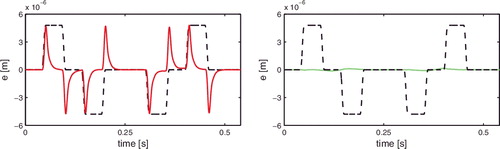
For the considered experimental setup in Section 7, the (normalised) a(t) of a typical r(t) is depicted in Figure 3, together with ${\widehat{e}}^{j+1}(t,{\theta }_a)$ based on (1) θ_a = 0 (red), and (2) the minimiser ${\widehat{\theta }}_a$ of V(θ_a) in (18(18) $$\begin{array}{c}\hfill V\left({\theta }_a\right)={\left|\left|\frac{1}{N}\sum _{t=1}^{N}a\left(t\right){\widehat{e}}^{j+1}(t,{\theta }_a)\right|\right|}^2,\end{array}$$(18) ) (green). Clearly, high performance is obtained with ${\widehat{\theta }}_a$, i.e. when a(t) and ${\widehat{e}}^{j+1}(t,{\theta }_a)$ are uncorrelated. In contrast, low performance is obtained for θ_a = 0, which corresponds to significant correlation between a(t) and ${\widehat{e}}^{j+1}(t,{\theta }_a)$. This shows that the correlation between a(t) and ${\widehat{e}}^{j+1}(t,{\theta }_a)$ is a measure for the performance of a motion system.

Figure 3. Tuning of a feedforward controller for a motion system. Low performance in an instrumental variable framework: significant correlation between the acceleration a(t) (dashed black) and predicted error ${\widehat{e}}^{j+1}(t,{\theta }_a)$ (red) for θ_a = 0 (left). High performance in an instrumental variable framework: a(t) (dashed black) and ${\widehat{e}}^{j+1}(t,{\theta }_a)$ (green) are uncorrelated for the minimiser ${\widehat{\theta }}_a$ of the criterion V(θ_a) in (18(18) $$\begin{array}{c}\hfill V\left({\theta }_a\right)={\left|\left|\frac{1}{N}\sum _{t=1}^{N}a\left(t\right){\widehat{e}}^{j+1}(t,{\theta }_a)\right|\right|}^2,\end{array}$$(18) ) (right). (To view this figure in colour, please see the online version of the journal).

Next, the asymptotic covariance matrix P_IV is derived that is related to ${\widehat{\theta }}^{\Delta }$. Consider the asymptotic distribution of ${\widehat{\theta }}^{\Delta }$ given by (19) $$\begin{array}{c}\hfill \sqrt{N}({\widehat{\theta }}^{\Delta }-{\theta }_0^{\Delta })\stackrel{\text{dist}}{\to }\mathcal{N}(0,P_{IV}),\end{array}$$(19) where θ^Δ₀ is the asymptotic parameter estimate as defined in (15(15) $$\begin{array}{c}\hfill e_m^j\left(t\right)={\left({\varphi }^j\left(t\right)\right)}^T{\theta }_0^{\Delta }-e_w^j\left(t\right).\end{array}$$(15) ). It can be shown that ${\widehat{\theta }}^{\Delta }$ is a consistent estimator, i.e. ${\widehat{\theta }}^{\Delta }$ converges to θ^Δ₀ for N to infinity, along similar lines as in, e.g. Söderström, Stoica, and Trulsson (1987). Then, the asymptotic covariance matrix P_IV in (19(19) $$\begin{array}{c}\hfill \sqrt{N}({\widehat{\theta }}^{\Delta }-{\theta }_0^{\Delta })\stackrel{\text{dist}}{\to }\mathcal{N}(0,P_{IV}),\end{array}$$(19) ) is given by (20) $$\begin{array}{c}\hfill P_{IV}={\left(R_{z{\varphi }^j}^{T}W{R}_{z{\varphi }^j}\right)}^{-1}{R}_{z{\varphi }^j}^{T}WJ{W}^T{R}_{z{\varphi }^j}{\left(R_{z{\varphi }^j}^{T}W{R}_{z{\varphi }^j}\right)}^{-T},\end{array}$$(20) with (21) $$\begin{array}{c}\hfill \begin{array}{cc}\hfill R_{z{\varphi }^j}& =\bar{\mathbb{E}}z\left(t\right)L\left(q\right){\left({\varphi }_r^j\left(t\right)\right)}^T,\hfill \\ \hfill J& ={\lambda }_{\epsilon }^2\bar{\mathbb{E}}\left[L\left(q\right)z\left(t\right)\right]{\left[L\left(q\right)z\left(t\right)\right]}^T,\hfill \end{array}\end{array}$$(21) and reference-induced part ϕ^j_r(t) of ϕ^j(t) in (13(13) $$\begin{array}{c}\hfill {\varphi }^j\left(t\right)=\Psi \left(q\right){(C_{fb}\left(q\right)+C_{ff}^j\left(q\right))}^{-1}{y}_m^j\left(t\right)\in {\mathbb{R}}^{n_{\theta }}.\end{array}$$(13) ) given by (22) $$\begin{array}{c}\hfill {\varphi }_r^j\left(t\right)=\Psi \left(q\right){(C_{fb}\left(q\right)+C_{ff}^j\left(q\right))}^{-1}{y}_r^j\left(t\right),\end{array}$$(22) with y^j_r(t) as in (2(2) $$\begin{array}{c}\hfill \begin{array}{c}{e}_r^j\left(t\right)=S\left(q\right)(1-P\left(q\right)C_{ff}^j\left(q\right))r\left(t\right),\hfill \\ e_w^j=S\left(q\right)w^j\left(t\right),\hfill \\ y_r^j\left(t\right)=S\left(q\right)P\left(q\right)(C_{fb}\left(q\right)+C_{ff}^j\left(q\right))r\left(t\right),\hfill \\ y_w^j=S\left(q\right)w^j\left(t\right),\hfill \end{array}\end{array}$$(2) ). A derivation of (20(20) $$\begin{array}{c}\hfill P_{IV}={\left(R_{z{\varphi }^j}^{T}W{R}_{z{\varphi }^j}\right)}^{-1}{R}_{z{\varphi }^j}^{T}WJ{W}^T{R}_{z{\varphi }^j}{\left(R_{z{\varphi }^j}^{T}W{R}_{z{\varphi }^j}\right)}^{-T},\end{array}$$(20) ) for iterative feedforward control follows the proof derived in Söderström and Stoica (1989, App. A8.1) for open-loop identification, and Söderström et al. (1987, Section 3) for closed-loop identification.

Note that P_IV in (20(20) $$\begin{array}{c}\hfill P_{IV}={\left(R_{z{\varphi }^j}^{T}W{R}_{z{\varphi }^j}\right)}^{-1}{R}_{z{\varphi }^j}^{T}WJ{W}^T{R}_{z{\varphi }^j}{\left(R_{z{\varphi }^j}^{T}W{R}_{z{\varphi }^j}\right)}^{-T},\end{array}$$(20) ) depends on the design of z(t) and L(q). Next, a lower bound is derived for P_IV as a function of z(t) and L(q), which corresponds to the minimum variance achievable with an IV method for feedforward control.

3.3 Optimal design procedure for z(t) and L(q)

The covariance matrix P_IV in (20(20) $$\begin{array}{c}\hfill P_{IV}={\left(R_{z{\varphi }^j}^{T}W{R}_{z{\varphi }^j}\right)}^{-1}{R}_{z{\varphi }^j}^{T}WJ{W}^T{R}_{z{\varphi }^j}{\left(R_{z{\varphi }^j}^{T}W{R}_{z{\varphi }^j}\right)}^{-T},\end{array}$$(20) ) depends on the design of z(t) and L(q). Optimal accuracy in terms of variance is obtained if z(t) and L(q) are designed such that P_IV is equal to an optimal covariance matrix $P_{IV}^{\text{opt}}$, where for any z(t) and L(q), it holds that $P_{IV}⪰P_{IV}^{\text{opt}}.$ The optimal covariance matrix $P_{IV}^{\text{opt}}$ for iterative feedforward control based on instrumental variables is given by (23) $$\begin{array}{c}\hfill P_{IV}^{\text{opt}}={\lambda }_{\epsilon }^2{\left\{\bar{\mathbb{E}}{\varphi }_r^j\left(t\right){\left({\varphi }_r^j\left(t\right)\right)}^T\right\}}^{-1},\end{array}$$(23) where $P_{IV}^{\text{opt}}\succ 0$. A derivation of $P_{IV}^{\text{opt}}$ follows along similar lines as the derivation for open-loop identification in Söderström and Stoica (1989, Chapter 8).

Equivalence between P_IV in (20(20) $$\begin{array}{c}\hfill P_{IV}={\left(R_{z{\varphi }^j}^{T}W{R}_{z{\varphi }^j}\right)}^{-1}{R}_{z{\varphi }^j}^{T}WJ{W}^T{R}_{z{\varphi }^j}{\left(R_{z{\varphi }^j}^{T}W{R}_{z{\varphi }^j}\right)}^{-T},\end{array}$$(20) ) and $P_{IV}^{\text{opt}}$ in (23(23) $$\begin{array}{c}\hfill P_{IV}^{\text{opt}}={\lambda }_{\epsilon }^2{\left\{\bar{\mathbb{E}}{\varphi }_r^j\left(t\right){\left({\varphi }_r^j\left(t\right)\right)}^T\right\}}^{-1},\end{array}$$(23) ) holds if z(t), L(q) and W are designed as (24) $$\begin{array}{cc}& z_{\text{opt}}\left(t\right)={\varphi }_r^j\left(t\right),\hfill \\ & L_{\text{opt}}\left(q\right)=1,\hfill \\ & W_{\text{opt}}=I,\text{and}{n}_z=n_{\theta },\hfill \end{array}$$(24) and ϕ^j_r(t) in (22(22) $$\begin{array}{c}\hfill {\varphi }_r^j\left(t\right)=\Psi \left(q\right){(C_{fb}\left(q\right)+C_{ff}^j\left(q\right))}^{-1}{y}_r^j\left(t\right),\end{array}$$(22) ). This result follows by substituting z_opt(t), L_opt(q), and W_opt in (20(20) $$\begin{array}{c}\hfill P_{IV}={\left(R_{z{\varphi }^j}^{T}W{R}_{z{\varphi }^j}\right)}^{-1}{R}_{z{\varphi }^j}^{T}WJ{W}^T{R}_{z{\varphi }^j}{\left(R_{z{\varphi }^j}^{T}W{R}_{z{\varphi }^j}\right)}^{-T},\end{array}$$(20) ). Note that this design is not unique, and closely related to the proposed instrumental variables in the RIV algorithms.

The following two observations are made based on z_opt(t), L_opt(q), and W_opt. First, the optimal design reveals that minimum variance is obtained when the number of instruments n_z is equal to the number of parameters n_θ, and uniform weighting (W = I) is applied for t = 1, ..., N. Based on this observation, W and n_z are furthermore selected as W = I and n_z = n_θ. Then, (20(20) $$\begin{array}{c}\hfill P_{IV}={\left(R_{z{\varphi }^j}^{T}W{R}_{z{\varphi }^j}\right)}^{-1}{R}_{z{\varphi }^j}^{T}WJ{W}^T{R}_{z{\varphi }^j}{\left(R_{z{\varphi }^j}^{T}W{R}_{z{\varphi }^j}\right)}^{-T},\end{array}$$(20) ) becomes (25) $$\begin{array}{c}\hfill P_{IV}=R_{z{\varphi }^j}^{-1}J{R}_{z{\varphi }^j}^{-T},\end{array}$$(25) with $R_{z{\varphi }^j}$ and J as in (21(21) $$\begin{array}{c}\hfill \begin{array}{cc}\hfill R_{z{\varphi }^j}& =\bar{\mathbb{E}}z\left(t\right)L\left(q\right){\left({\varphi }_r^j\left(t\right)\right)}^T,\hfill \\ \hfill J& ={\lambda }_{\epsilon }^2\bar{\mathbb{E}}\left[L\left(q\right)z\left(t\right)\right]{\left[L\left(q\right)z\left(t\right)\right]}^T,\hfill \end{array}\end{array}$$(21) ). Furthermore, (17(17) $$\begin{array}{c}\hfill {\widehat{\theta }}^{\Delta }={\left({\widehat{R}}_{z{\varphi }^j}^{T}W{\widehat{R}}_{z{\varphi }^j}\right)}^{-1}{\widehat{R}}_{z{\varphi }^j}^{T}W{\widehat{R}}_{z{e}_m^j},\end{array}$$(17) ) reduces to a basic IV method, i.e. (26) $$\begin{array}{c}\hfill {\widehat{\theta }}^{\Delta }={\widehat{R}}_{z{\varphi }^j}^{-1}{\widehat{R}}_{z{e}_m^j}.\end{array}$$(26)

Second, the optimal instruments z_opt(t) cannot be determined since P(q) is assumed to be unknown in the developed framework. To see this, note that ϕ^j_r(t) in (22(22) $$\begin{array}{c}\hfill {\varphi }_r^j\left(t\right)=\Psi \left(q\right){(C_{fb}\left(q\right)+C_{ff}^j\left(q\right))}^{-1}{y}_r^j\left(t\right),\end{array}$$(22) ), and in particular y^j_r(t), cannot be determined based on the known r(t), and measured e^j_m(t) and y^j_m(t) when P(q) is unknown. In the next section, a novel algorithm is proposed that alternates between iteratively updating the estimate of the noise-free z_opt(t), and determining ${\widehat{\theta }}^{\Delta }$, similar to the algorithms described in Young (2015).

4. Proposed approach achieving optimal accuracy

4.1 Proposed RIV algorithm

The algorithm proposed in this section is an iterative method to achieve optimal accuracy by jointly updating the estimate of the optimal instruments z_opt(t) in (24(24) $$\begin{array}{cc}& z_{\text{opt}}\left(t\right)={\varphi }_r^j\left(t\right),\hfill \\ & L_{\text{opt}}\left(q\right)=1,\hfill \\ & W_{\text{opt}}=I,\text{and}{n}_z=n_{\theta },\hfill \end{array}$$(24) ) and solving for ${\widehat{\theta }}^{\Delta }$ as in (26(26) $$\begin{array}{c}\hfill {\widehat{\theta }}^{\Delta }={\widehat{R}}_{z{\varphi }^j}^{-1}{\widehat{R}}_{z{e}_m^j}.\end{array}$$(26) ). Note that measured data from a single task is sufficient. Related iterative RIV methods are developed in system identification (see Jakeman & Young (1979); Young, 2015; Young & Jakeman (1979, 1980).

Let the index i denote the ith computational iteration of the proposed algorithm. Furthermore, ${\widehat{\theta }}_{<i-1>}^{\Delta }$ denotes the parameter estimate in iteration i − 1. In the ith iteration, z_opt(t) is approximated by (27) $$\begin{array}{cc}\hfill z_{\text{p},<i>}\left(t\right)& ={\widehat{\varphi }}_r^j\left(t\right):=\Psi \left(q\right)(C_{fb}\left(q\right)\hfill \\ & +C_{ff,<i>}^j\left(q,{\widehat{\theta }}_{<i-1>}^{\Delta }\right){)}^{-1}r\left(t\right).\hfill \end{array}$$(27) Subsequently, z_{p, <i >}(t) in (27(27) $$\begin{array}{cc}\hfill z_{\text{p},<i>}\left(t\right)& ={\widehat{\varphi }}_r^j\left(t\right):=\Psi \left(q\right)(C_{fb}\left(q\right)\hfill \\ & +C_{ff,<i>}^j\left(q,{\widehat{\theta }}_{<i-1>}^{\Delta }\right){)}^{-1}r\left(t\right).\hfill \end{array}$$(27) ) is used to determine ${\widehat{\theta }}_{<i>}^{\Delta }$ in the ith iteration similar to (26(26) $$\begin{array}{c}\hfill {\widehat{\theta }}^{\Delta }={\widehat{R}}_{z{\varphi }^j}^{-1}{\widehat{R}}_{z{e}_m^j}.\end{array}$$(26) ): $$\begin{array}{c}\hfill {\widehat{\theta }}_{<i>}^{\Delta }={\left({\widehat{R}}_{z{\varphi }^j,<i>}\right)}^{-1}{\widehat{R}}_{z{e}_m^j,<i>},\end{array}$$ where ${\widehat{R}}_{z{\varphi }^j,<i>}=\frac{1}{N}{\sum }_{t=1}^N{z}_{\text{p},<i>}\left(t\right){\left({\varphi }^j\left(t\right)\right)}^T$ with ϕ^j(t) in (13(13) $$\begin{array}{c}\hfill {\varphi }^j\left(t\right)=\Psi \left(q\right){(C_{fb}\left(q\right)+C_{ff}^j\left(q\right))}^{-1}{y}_m^j\left(t\right)\in {\mathbb{R}}^{n_{\theta }}.\end{array}$$(13) ), and ${\widehat{R}}_{z{e}_m^j,<i>}=\frac{1}{N}{\sum }_{t=1}^N{z}_{\text{p},<i>}\left(t\right)e_m^j\left(t\right)$ with e^j_m(t) in (1(1) $$\begin{array}{c}\hfill \begin{array}{c}\hfill e_m^j\left(t\right)=e_r^j\left(t\right)-e_w^j\left(t\right),\\ \hfill y_m^j\left(t\right)=y_r^j\left(t\right)+y_w^j\left(t\right),\end{array}\end{array}$$(1) ). The proposed algorithm to determine ${\widehat{\theta }}^{\Delta }$ with optimal accuracy is summarised in Algorithm 4.1.

Algorithm 4.1:

Determine ${\widehat{\theta }}^{\Delta }$ with optimal accuracy

(a)	Initialise ${\widehat{\theta }}_{<i-1>}^{\Delta }=0$.
(b)	Construct  $C_{ff,<i>}^j(q,{\widehat{\theta }}_{<i-1>}^{\Delta })=\Psi \left(q\right)({\theta }^j+{\widehat{\theta }}_{<i-1>}^{\Delta }).$
(c)	Construct instrumental variables $z_{\text{p},<i>}\left(t\right)=\Psi \left(q\right){(C_{fb}\left(q\right)+C_{ff,<i>}^j(q,{\widehat{\theta }}_{<i-1>}^{\Delta }))}^{-1}r\left(t\right)$.
(d)	Determine ${\widehat{R}}_{z{\varphi }^j,<i>}=\frac{1}{N}{\sum }_{t=1}^N{z}_{\text{p},<i>}\left(t\right){\left({\varphi }^j\left(t\right)\right)}^T$ and ${\widehat{R}}_{z{e}_m^j,<i>}=\frac{1}{N}{\sum }_{t=1}^N{z}_{\text{p},<i>}\left(t\right)e_m^j\left(t\right),$ based on ϕj(t) in (13(13) $$\begin{array}{c}\hfill {\varphi }^j\left(t\right)=\Psi \left(q\right){(C_{fb}\left(q\right)+C_{ff}^j\left(q\right))}^{-1}{y}_m^j\left(t\right)\in {\mathbb{R}}^{n_{\theta }}.\end{array}$$(13) ) and ejm(t) in (1(1) $$\begin{array}{c}\hfill \begin{array}{c}\hfill e_m^j\left(t\right)=e_r^j\left(t\right)-e_w^j\left(t\right),\\ \hfill y_m^j\left(t\right)=y_r^j\left(t\right)+y_w^j\left(t\right),\end{array}\end{array}$$(1) ).
(e)	Solve for ${\widehat{\theta }}_{<i>}^{\Delta }$ as in (26(26) $$\begin{array}{c}\hfill {\widehat{\theta }}^{\Delta }={\widehat{R}}_{z{\varphi }^j}^{-1}{\widehat{R}}_{z{e}_m^j}.\end{array}$$(26) ): ${\widehat{\theta }}_{<i>}^{\Delta }={\left({\widehat{R}}_{z{\varphi }^j,<i>}\right)}^{-1}{\widehat{R}}_{z{e}_m^j,<i>}.$
(f)	Set i → i + 1 and repeat from Step (b) until a stopping criterion is met.
(g)	Set ${\widehat{\theta }}^{\Delta }={\widehat{\theta }}_{<i>}^{\Delta }$.

Before initiating Algorithm 4.1, it is advised to determine an initial parameter θ^j by using a linear least squares estimation approach as in van der Meulen et al. (2008). Similar to the RIV algorithms presented in Young (2015), practical use has shown that such an initial estimate is typically sufficient for subsequent convergence of Algorithm 4.1.

Remark 4.1:

An approach to deal with possible instability of ${(C_{fb}\left(q\right)+C_{ff,<i>}^j(q,{\widehat{\theta }}_{<i-1>}^{\Delta }))}^{-1}$ in computing z_{p, <i >}(t) is given in Boeren, Oomen, et al. (2015, Appendix A).

4.2 Accuracy analysis of the proposed approach

In this section, it is shown that optimal accuracy in terms of accuracy is obtained with Algorithm 4.1. Consider the covariance matrix P_{IV, p} corresponding to z_{p, <i >}(t) as given in Table 1. The covariance P_{IV, p} follows by substituting (27(27) $$\begin{array}{cc}\hfill z_{\text{p},<i>}\left(t\right)& ={\widehat{\varphi }}_r^j\left(t\right):=\Psi \left(q\right)(C_{fb}\left(q\right)\hfill \\ & +C_{ff,<i>}^j\left(q,{\widehat{\theta }}_{<i-1>}^{\Delta }\right){)}^{-1}r\left(t\right).\hfill \end{array}$$(27) ) in (25(25) $$\begin{array}{c}\hfill P_{IV}=R_{z{\varphi }^j}^{-1}J{R}_{z{\varphi }^j}^{-T},\end{array}$$(25) ). Clearly, optimal accuracy for the proposed method, i.e. P_{IV, p} equal to $P_{IV}^{\text{opt}}$ in (23(23) $$\begin{array}{c}\hfill P_{IV}^{\text{opt}}={\lambda }_{\epsilon }^2{\left\{\bar{\mathbb{E}}{\varphi }_r^j\left(t\right){\left({\varphi }_r^j\left(t\right)\right)}^T\right\}}^{-1},\end{array}$$(23) ), is obtained if z_{p, <i >}(t) converges to z_opt(t) in Algorithm 4.1.

Table 1. The comparison study presented in Sections 4 and 5 of this paper shows that optimal accuracy is not achieved with the existing approaches in van der Meulen et al. (2008) and Boeren, Oomen, et al. (2015) while the proposed approach can achieve optimal accuracy upon convergence of the proposed RIV algorithm.

Method	Instrumental	Covariance matrix PIV	Optimal
	variables		accuracy
Optimal	$z_{\text{opt}}\left(t\right)={\varphi }_r^j\left(t\right)$	$P_{IV}^{\text{opt}}={\lambda }_{\epsilon }^2{\left[\bar{\mathbb{E}}{\varphi }_r^j\left(t\right){\left({\varphi }_r^j\left(t\right)\right)}^T\right]}^{-1}$	Yes
Proposed (Section 4)	$z_{\text{p},<i>}\left(t\right)={\widehat{\varphi }}_r^j\left(t\right)$	$P_{IV,p}={\lambda }_{\epsilon }^2{\left[\bar{\mathbb{E}}{\widehat{\varphi }}_r^j\left(t\right){\left({\varphi }_r^j\left(t\right)\right)}^T\right]}^{-1}\times$	Yes
		$\left[\bar{\mathbb{E}}{\widehat{\varphi }}_r^j\left(t\right){\left({\widehat{\varphi }}_r^j\left(t\right)\right)}^T\right]{\left[\bar{\mathbb{E}}{\widehat{\varphi }}_r^j\left(t\right){\left({\varphi }_r^j\left(t\right)\right)}^T\right]}^{-T}$
Method 1 (Section 5.1)	z1(t) = Ψ(q)r(t)	$P_{IV,1}={\lambda }_{\epsilon }^2{\left[\bar{\mathbb{E}}\Psi r\left(t\right){\left({\varphi }_r^j\left(t\right)\right)}^T\right]}^{-1}\times$	No, arbitrary
		$\left[\bar{\mathbb{E}}\Psi r\left(t\right){\left(\Psi r\left(t\right)\right)}^T\right]{\left[\bar{\mathbb{E}}\Psi r\left(t\right){\left({\varphi }_r^j\left(t\right)\right)}^T\right]}^{-T}$
Method 2 (Section 5.2)	z2(t) = ϕ2(t)	$P_{IV,2}={\lambda }_{\epsilon }^2{\left[\bar{\mathbb{E}}{\varphi }_r\left(t\right){\left({\varphi }_r^j\left(t\right)\right)}^T\right]}^{-1}\times$	No, $\sqrt{2}$
		$\left[\bar{\mathbb{E}}{\varphi }_2\left(t\right){\varphi }_2^T\left(t\right)\right]{\left[\bar{\mathbb{E}}{\varphi }_r\left(t\right){\left({\varphi }_r^j\left(t\right)\right)}^T\right]}^{-T}$

To show that z_{p, <i >}(t) converges to z_opt(t) in subsequent iterations of the proposed algorithm, substitute (2(2) $$\begin{array}{c}\hfill \begin{array}{c}{e}_r^j\left(t\right)=S\left(q\right)(1-P\left(q\right)C_{ff}^j\left(q\right))r\left(t\right),\hfill \\ e_w^j=S\left(q\right)w^j\left(t\right),\hfill \\ y_r^j\left(t\right)=S\left(q\right)P\left(q\right)(C_{fb}\left(q\right)+C_{ff}^j\left(q\right))r\left(t\right),\hfill \\ y_w^j=S\left(q\right)w^j\left(t\right),\hfill \end{array}\end{array}$$(2) ) and (22(22) $$\begin{array}{c}\hfill {\varphi }_r^j\left(t\right)=\Psi \left(q\right){(C_{fb}\left(q\right)+C_{ff}^j\left(q\right))}^{-1}{y}_r^j\left(t\right),\end{array}$$(22) ) in (24(24) $$\begin{array}{cc}& z_{\text{opt}}\left(t\right)={\varphi }_r^j\left(t\right),\hfill \\ & L_{\text{opt}}\left(q\right)=1,\hfill \\ & W_{\text{opt}}=I,\text{and}{n}_z=n_{\theta },\hfill \end{array}$$(24) ) to obtain (28) $$\begin{array}{cc}\hfill z_{\text{opt}}\left(t\right)& =\Psi \left(q\right){(C_{fb}\left(q\right)+C_{ff}^j\left(q\right))}^{-1}{y}_r^j\left(t\right)\hfill \\ & =\Psi \left(q\right){(C_{fb}\left(q\right)+C_{ff}^j\left(q\right))}^{-1}S\left(q\right)P\left(q\right)(C_{fb}\left(q\right)\hfill \\ & +C_{ff}^j\left(q\right))r\left(t\right)\hfill \\ & =\Psi \left(q\right)S\left(q\right)P\left(q\right)r\left(t\right),\hfill \end{array}$$(28) where the last equality is obtained by using the commutative property of SISO systems. Then, the difference between z_opt(t) and z_{p, <i >}(t) in the ith iteration can be expressed as $$\begin{array}{ccc}& & z_{\text{opt}}\left(t\right)-z_{\text{p},<i>}\left(t\right)\hfill \\ & =& \Psi \left(q\right)\left(S\right(q\left)P\right(q)\hfill \\ & & -{\left(C_{fb}\left(q\right)+C_{ff,<i>}^j\left(q,{\widehat{\theta }}_{<i-1>}^{\Delta }\right)\right)}^{-1})r\left(t\right),\hfill \end{array}$$ and z_{p, <i >}(t) = z_opt(t), i.e. optimal accuracy, is obtained if (29) $$\begin{array}{c}\hfill {(C_{fb}\left(q\right)+C_{ff,<i>}^j(q,{\widehat{\theta }}_{<i-1>}^{\Delta }))}^{-1}=S\left(q\right)P\left(q\right).\end{array}$$(29)

It remains to be shown that (31(31) $$\begin{array}{ccc}\hfill P_{IV,1}& =& {\lambda }_{\epsilon }^2{\left[\bar{\mathbb{E}}\Psi \left(q\right)r\left(t\right){\left({\varphi }_r^j\left(t\right)\right)}^T\right]}^{-1}\hfill \\ & & \times \left[\bar{\mathbb{E}}\Psi \left(q\right)r\left(t\right){\left(\Psi \left(q\right)r\left(t\right)\right)}^T\right]\hfill \\ & & \times {\left[\bar{\mathbb{E}}\Psi \left(q\right)r\left(t\right){\left({\varphi }_r^j\left(t\right)\right)}^T\right]}^{-T}.\hfill \end{array}$$(31) ) holds, i.e. z_{p, <i >}(t) converges to z_opt(t), to guarantee that Algorithm 4.1 results in optimal accuracy. Recall from Section 3 that ${\widehat{\theta }}_{<1>}^{\Delta }$ in iteration i = 1 is a consistent estimator, i.e. ${\widehat{\theta }}_{<1>}^{\Delta }={\theta }_0^{\Delta }$ for N to infinity, and that consistency of ${\widehat{\theta }}_{<1>}^{\Delta }$ implies that (30) $$\begin{array}{c}\hfill C_{ff,<2>}^j(q,{\widehat{\theta }}_{<1>}^{\Delta })=P^{-1}\left(q\right).\end{array}$$(30) Substituting (29(29) $$\begin{array}{c}\hfill {(C_{fb}\left(q\right)+C_{ff,<i>}^j(q,{\widehat{\theta }}_{<i-1>}^{\Delta }))}^{-1}=S\left(q\right)P\left(q\right).\end{array}$$(29) ) in (29(29) $$\begin{array}{c}\hfill {(C_{fb}\left(q\right)+C_{ff,<i>}^j(q,{\widehat{\theta }}_{<i-1>}^{\Delta }))}^{-1}=S\left(q\right)P\left(q\right).\end{array}$$(29) ) with i = 2 and rearranging terms illustrates that z_{p, <2 >}(t) = z_opt(t). This result shows that optimal accuracy in terms of accuracy is achieved with Algorithm 4.1.

Remark 4.2:

For finite N, ${\widehat{\theta }}_{<1>}^{\Delta }$ is not exactly equal to θ^Δ₀ and multiple iterations are typically required to refine z_{p, <i >}(t). Practical use of the algorithm shows good convergence properties. This is in accordance with the convergence analysis for closely related iterative RIV algorithms (Young, 2015).

4.3 Design procedure

Next, Algorithm 4.1 is embedded in a design procedure to determine C^{j + 1}_ff(q, θ^{j + 1}) according to (7(7) $$\begin{array}{c}\hfill {\widehat{\theta }}^{\Delta }=arg\underset{{\theta }^{\Delta }}{min}V\left({\theta }^{\Delta }\right),\end{array}$$(7) ) with V(θ^Δ) in (16(16) $$\begin{array}{c}\hfill V\left({\theta }^{\Delta }\right)={\left|\left|\frac{1}{N}\sum _{t=1}^{N}z\left(t\right)L\left(q\right){\widehat{e}}^{j+1}(t,{\theta }^{\Delta })\right|\right|}_W^2,\end{array}$$(16) ). This design procedure implements the main contribution of this paper, and is given next.

Procedure 4.1:

Estimation of C^{j + 1}_ff(q, θ^{j + 1}) after the jth task:

1.	Measure ejm(t) and yjm(t) for $t=1,\cdots ,N$, in the jth task.
2.	Construct ϕj(t) = Ψ(q)(Cfb(q) + Cjff(q, θj))− 1yjm(t).
3.	Algorithm 4.1: Determine ${\widehat{\theta }}^{\Delta }$ with optimal accuracy.
4.	Construct $C_{ff}^{j+1}(q,{\theta }^{j+1})=\Psi \left(q\right)({\theta }^j+{\widehat{\theta }}^{\Delta }).$
5.	Set j → j + 1 and go to Step 1.

Remark 4.3:

Procedure 4.1 is based on measured data from a single task. The proposed procedure can directly be implemented as a (batch-wise) recursive approach, where measured data from multiple tasks is used to reduce the variance of ${\widehat{\theta }}^{\Delta }$.

5. Accuracy analysis of existing approaches

In this section, the accuracy properties of the iterative feedforward tuning approaches in van der Meulen et al. (2008) and Boeren, Oomen, et al. (2015) are compared with the optimal approach derived in Section 3. An overview of this comparison is provided in Table 1.

5.1 Accuracy analysis of the approach in Boeren, Oomen, et al. (2015)

The instrumental variable approach in Boeren, Oomen, et al. (2015) uses as instruments z₁(t) = Ψ(q)r(t), with Ψ(q) the basis functions of C^j_ff(q), and L₁(q) = 1. The covariance matrix P_{IV, 1} corresponding to this design follows by substituting z₁(t) and L₁(q) = 1 in (25(25) $$\begin{array}{c}\hfill P_{IV}=R_{z{\varphi }^j}^{-1}J{R}_{z{\varphi }^j}^{-T},\end{array}$$(25) ), and is given by (31) $$\begin{array}{ccc}\hfill P_{IV,1}& =& {\lambda }_{\epsilon }^2{\left[\bar{\mathbb{E}}\Psi \left(q\right)r\left(t\right){\left({\varphi }_r^j\left(t\right)\right)}^T\right]}^{-1}\hfill \\ & & \times \left[\bar{\mathbb{E}}\Psi \left(q\right)r\left(t\right){\left(\Psi \left(q\right)r\left(t\right)\right)}^T\right]\hfill \\ & & \times {\left[\bar{\mathbb{E}}\Psi \left(q\right)r\left(t\right){\left({\varphi }_r^j\left(t\right)\right)}^T\right]}^{-T}.\hfill \end{array}$$(31) Based on (31(31) $$\begin{array}{ccc}\hfill P_{IV,1}& =& {\lambda }_{\epsilon }^2{\left[\bar{\mathbb{E}}\Psi \left(q\right)r\left(t\right){\left({\varphi }_r^j\left(t\right)\right)}^T\right]}^{-1}\hfill \\ & & \times \left[\bar{\mathbb{E}}\Psi \left(q\right)r\left(t\right){\left(\Psi \left(q\right)r\left(t\right)\right)}^T\right]\hfill \\ & & \times {\left[\bar{\mathbb{E}}\Psi \left(q\right)r\left(t\right){\left({\varphi }_r^j\left(t\right)\right)}^T\right]}^{-T}.\hfill \end{array}$$(31) ) and (23(23) $$\begin{array}{c}\hfill P_{IV}^{\text{opt}}={\lambda }_{\epsilon }^2{\left\{\bar{\mathbb{E}}{\varphi }_r^j\left(t\right){\left({\varphi }_r^j\left(t\right)\right)}^T\right\}}^{-1},\end{array}$$(23) ), it can be shown that $P_{IV,1}\succ P_{IV}^{\text{opt}},$ i.e. the approach in Boeren, Oomen, et al. (2015) results in non-optimal accuracy in terms of variance.

5.2 Accuracy analysis of the approach in van der Meulen et al. (2008)

The iterative feedforward approach proposed in van der Meulen et al. (2008) utilises L₂(q) = 1 and z₂(t) = ϕ₂(t) as instruments, where ϕ₂(t) = Ψ(q)(C_fb(q) + C^j_ff(q))^{− 1}y_m(t) is constructed based on measured data obtained in an additional task. As such, measured data from two tasks is required to determine ${\widehat{\theta }}^{\Delta }$, which results in a $1/\sqrt{2}$ reduced accuracy compared to the optimal approach in Section 3. To see this, note that the asymptotic distribution of ${\widehat{\theta }}^{\Delta }$ corresponding to z₂(t) yields (32) $$\begin{array}{c}\hfill \sqrt{N}({\widehat{\theta }}^{\Delta }-{\theta }_0^{\Delta })\stackrel{\text{dist}}{\to }\mathcal{N}(0,P_{IV,2}),\end{array}$$(32) based on two tasks of each N samples, where P_{IV, 2} yields $$\begin{array}{ccc}\hfill P_{IV,2}& =& {\lambda }_{\epsilon }^2{\left[\bar{\mathbb{E}}{\varphi }_r^j\left(t\right){\left({\varphi }_r^j\left(t\right)\right)}^T\right]}^{-1}\hfill \\ & & \times \left[\bar{\mathbb{E}}{\varphi }_2\left(t\right){\varphi }_2^T\left(t\right)\right]{\left[\bar{\mathbb{E}}{\varphi }_r^j\left(t\right){\left({\varphi }_r^j\left(t\right)\right)}^T\right]}^{-T}.\hfill \end{array}$$ In contrast, the asymptotic distribution corresponding to the optimal instruments z_opt is given by (33) $$\begin{array}{c}\hfill \sqrt{2N}({\widehat{\theta }}^{\Delta }-{\theta }_0^{\Delta })\stackrel{\text{dist}}{\to }\mathcal{N}(0,P_{IV}^{\text{opt}}),\end{array}$$(33) based on two tasks of each N samples. Comparing (32(34) $$\begin{array}{c}\hfill {\bar{\theta }}^j={\displaystyle \frac{1}{m}}\sum _{l=1}^m{\widehat{\theta }}_l^j,\end{array}$$(34) ) and (33(33) $$\begin{array}{c}\hfill \sqrt{2N}({\widehat{\theta }}^{\Delta }-{\theta }_0^{\Delta })\stackrel{\text{dist}}{\to }\mathcal{N}(0,P_{IV}^{\text{opt}}),\end{array}$$(33) ) reveals a $1/\sqrt{2}$ reduced accuracy for the approach based on z₂(t) when compared to the optimal approach. This result confirms that non-optimal accuracy is obtained with the approach proposed in van der Meulen et al. (2008).

6. Simulation example

In this section, a simulation study is presented to

(1)	Confirm that unbiased parameter estimates are obtained for all considered IV approaches in Table 1,
(2)	Show that the proposed approach zp, <i >(t) leads to enhanced accuracy of the parameter estimates compared to the pre-existing approaches based on z1(t) and z2(t),
(3)	Illustrate the close relation between the statistical accuracy of ${\widehat{\theta }}^{\Delta }$ and the performance of a motion system.

6.1 System description

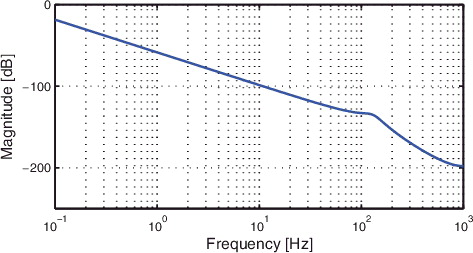
Consider the system P(q) given by $$\begin{array}{c}\hfill P\left(q\right)={\displaystyle \frac{1.761\times {10}^{-9}}{1-3.69q^{-1}+5.225q^{-2}-3.38q^{-3}+0.8451q^{-4}}},\end{array}$$ which represents a two-mass spring damper system with non-collocated dynamics (see Figure 4 for a Bode plot). A schematic illustration of the two-mass spring damper system is depicted in Figure 5. The feedback controller C_fb(q) is given by $$\begin{array}{c}\hfill C_{fb}={\displaystyle \frac{7.444\times {10}^4{q}^{-1}-1.47\times {10}^5{q}^{-2}+7.259\times {10}^4{q}^{-3}}{1-2.736q^{-1}+2.49q^{-2}-0.7537q^{-3}}}.\end{array}$$ Recall from Section 2.2 that the unknown disturbance w^j(t) is assumed to be given by w^j(t) = H(q)ε^j(t). Here, H(q) is designed such that Assumption 2.1 holds, i.e. H(q) = 1 + P(q)C_fb(q), and {ε^j(t)} is normally distributed white noise with zero mean and standard deviation λ_ε = 2.5 × 10⁻⁸. The system is excited by a third-order reference signal, designed as in Biagiotti and Melchiorri (2012). Furthermore, the feedforward controller C^j_ff(q, θ^j) is parametrised as $$\begin{array}{c}\hfill C_{ff}^j(q,{\theta }^j)={\psi }_a\left(q^{-1}\right){\theta }_a^j+{\psi }_s\left(q^{-1}\right){\theta }_s^j,\end{array}$$ with basis functions $$\begin{array}{c}\hfill {\psi }_a\left(q^{-1}\right)={\left({\displaystyle \frac{1-q^{-1}}{T_s}}\right)}^2,{\psi }_s\left(q^{-1}\right)={\left({\displaystyle \frac{1-q^{-1}}{T_s}}\right)}^4,\end{array}$$ parameters θ^j = [θ^j_a, θ_s^j]^T, and sampling time T_s = 5 × 10⁻⁴ s. Hence, C^j_ff(q, θ^j) consist of acceleration feedforward ψ_a(q^{− 1})θ^j_a and snap feedforward ψ_s(q^{− 1})θ^j_s. Straightforward computations reveal that the true parameter vector θ₀ of C^j_ff(q, θ^j), as defined in Section 3, is given by θ₀ = [22,  3 × 10⁻⁵]^T. This implies that the reference-induced contribution e^j_r(t) is equal to zero for all t when C^j_ff(q, θ₀) is used as feedforward controller.

Figure 4. Bode diagram of the system P.

Figure 5. Schematic illustration of a two-mass spring damper system.

A Monte Carlo simulation study is performed for the proposed approach with z_{p, <i >}(t) in (27(27) $$\begin{array}{cc}\hfill z_{\text{p},<i>}\left(t\right)& ={\widehat{\varphi }}_r^j\left(t\right):=\Psi \left(q\right)(C_{fb}\left(q\right)\hfill \\ & +C_{ff,<i>}^j\left(q,{\widehat{\theta }}_{<i-1>}^{\Delta }\right){)}^{-1}r\left(t\right).\hfill \end{array}$$(27) ) and the pre-existing approaches based on z₁(t) and z₂(t). The number of realisations is equal to m = 200, and a parameter estimate in the lth realisation is denoted ${\widehat{\theta }}_l$. In a single realisation, M = 5 tasks are performed, consisting of N = 6000 samples each. After the jth task in the lth realisation, Procedure 4.1 is used to determine ${\widehat{\theta }}_l^{j+1}$ based on θ^j_l, and the measured signals e^j_m and y^j_m in the jth task. The initial parameter vector is given by θ^init = [16, 1 × 10⁻⁵]^T. The sample mean corresponding to the jth task in the lth realisation is defined as (34) $$\begin{array}{c}\hfill {\bar{\theta }}^j={\displaystyle \frac{1}{m}}\sum _{l=1}^m{\widehat{\theta }}_l^j,\end{array}$$(34) with ${\bar{\theta }}^j={\left[{\bar{\theta }}_a^j{\bar{\theta }}_s^j\right]}^T.$ The corresponding feedforward controller is denoted as $C_{ff}^j(q,{\bar{\theta }}^j)$.

6.2 Simulation results: parameter estimation

The results of the Monte Carlo simulation study are given in Figure 6 and Table 2. The following observations are made:

Figure 6. Simulation results. Parameters $\widehat{\theta }$ as a function of tasks for m = 200 realisations for z₁(t) (left), z₂(t) (middle) and the proposed z_{p, <i >}(t) (right) show that the standard deviation of ${\widehat{\theta }}_a$ is comparable for all approaches, while the standard deviation of ${\widehat{\theta }}_s$ is significantly smaller for the proposed z_{p, <i >}(t) compared to z₁(t) and z₂(t).

(1)	Unbiased estimates of θ0, i.e. 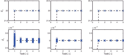${\bar{\theta }}^j={\theta }_0$, are obtained for zp, <i >(t), z1(t), and z2(t). This confirms that all considered IV approaches in Table 1 lead to unbiased estimates.
(2)	The standard deviation of ${\bar{\theta }}_s^j$ is significantly smaller for zp, <i >(t) when compared to z1(t) and z2(t). This confirms that the proposed approach leads to improved accuracy in terms of variance.

Table 2. Summary of results of Monte Carlo simulation. The mean value of ${\bar{\theta }}_a^1$ and ${\bar{\theta }}_s^1$ in task j = 1 for z_{p, <i >}(t), z₁(t) and z₂(t) confirm that unbiased parameter estimates are obtained for all methods, while the standard deviation of ${\bar{\theta }}_a^1$ and ${\bar{\theta }}_s^1$ confirms that an enhanced accuracy is obtained with the proposed approach z_{p, <i >}(t) compared to z₁(t) and z₂(t).

Method	Instrumental	Mean ${\bar{\theta }}_a^1$	Std. deviation ${\bar{\theta }}_a^1$	Mean ${\bar{\theta }}_s^1$	Std. deviation ${\bar{\theta }}_a^1$
	variables
Proposed (Section 4)	$z_{\text{p},<i>}\left(t\right)={\widehat{\varphi }}_r^j\left(t\right)$	22	2.2 × 10^−4	3 × 10^−5	1.2 × 10^−7
Method 1 (Section 5.1)	z1(t) = Ψ(q)r(t)	22	4.5 × 10^−4	3 × 10^−5	2.2 × 10^−6
Method 2 (Section 5.2)	z2(t) = ϕ2(t)	22	5.2 × 10^−4	3 × 10^−5	4.1 × 10^−7

6.3 Simulation results: accuracy and performance

Next, the relation between the statistical accuracy of the estimated parameters and the obtained performance is analysed for the considered system. Recall from (6(6) $$\begin{array}{c}\hfill e_r^{j+1}(t,{\theta }^{j+1})=S\left(q\right)(1-P\left(q\right)C_{ff}^{j+1}(q,{\theta }^{j+1}))r\left(t\right),\end{array}$$(6) ) that a high-performance C^j_ff(q, θ^j) minimises e^j_r(t, θ^j), i.e. the error induced by the known r(t). Since ${\bar{\theta }}^j$ in (34(34) $$\begin{array}{c}\hfill {\bar{\theta }}^j={\displaystyle \frac{1}{m}}\sum _{l=1}^m{\widehat{\theta }}_l^j,\end{array}$$(34) ) is an unbiased estimate of θ₀ for all approaches in Table 1, it follows from Section 3 that $e_r^j(t,{\bar{\theta }}^j)=0$ for all t when $C_{ff}^j(q,{\bar{\theta }}^j)$ is used as feedforward controller. Consequently, (1(1) $$\begin{array}{c}\hfill \begin{array}{c}\hfill e_m^j\left(t\right)=e_r^j\left(t\right)-e_w^j\left(t\right),\\ \hfill y_m^j\left(t\right)=y_r^j\left(t\right)+y_w^j\left(t\right),\end{array}\end{array}$$(1) ) implies that (35) $$\begin{array}{c}\hfill e_m^j(t,{\bar{\theta }}^j)=-e_w^j\left(t\right),\end{array}$$(35) which is the best possible result in the developed framework for a fixed C_fb(q). However, as already shown in Section 6.2, the estimate ${\widehat{\theta }}_l^j$ in realisation l can significantly deviate from the sample mean ${\bar{\theta }}^j$. In this section, the influence of this deviation on the achieved performance is analysed for the IV approaches in Table 1.

Suppose that ${\widehat{\theta }}_l^j$, $e_m^j(t,{\widehat{\theta }}_l^j)$ and $V\left({\widehat{\theta }}_l^j\right)$ are stored for all tasks, i.e. j = 1, …, 5, and all realisations, i.e. l = 1, …, 200. Let ${\widehat{\theta }}_{\mathrm{ wc }}^j$ denote the parameters such that $V\left({\widehat{\theta }}_{\mathrm{ wc }}^j\right)\ge V\left({\widehat{\theta }}_l^j\right)$ for l = 1, …, 200. The corresponding worst-case error $e_{\mathrm{ wc }}^j(t,{\widehat{\theta }}_{\mathrm{ wc }}^j)$ follows from (1(1) $$\begin{array}{c}\hfill \begin{array}{c}\hfill e_m^j\left(t\right)=e_r^j\left(t\right)-e_w^j\left(t\right),\\ \hfill y_m^j\left(t\right)=y_r^j\left(t\right)+y_w^j\left(t\right),\end{array}\end{array}$$(1) ) as (36) $$\begin{array}{c}\hfill e_{\mathrm{ wc }}^j(t,{\widehat{\theta }}_{\mathrm{ wc }}^j)=e_r^j(t,{\widehat{\theta }}_{\mathrm{ wc }}^j)-e_w^j\left(t\right),\end{array}$$(36) while the feedforward controller is denoted as $C_{ff}^j(q,{\widehat{\theta }}_{\text{wc}}^j)$. Next, it is shown that enhanced accuracy in terms of variance results in a smaller difference between $e_{\mathrm{ wc }}^j(t,{\widehat{\theta }}_{\mathrm{ wc }}^j)$ in (36(36) $$\begin{array}{c}\hfill e_{\mathrm{ wc }}^j(t,{\widehat{\theta }}_{\mathrm{ wc }}^j)=e_r^j(t,{\widehat{\theta }}_{\mathrm{ wc }}^j)-e_w^j\left(t\right),\end{array}$$(36) ) and $e_m^j(t,{\bar{\theta }}^j)$ in (35(35) $$\begin{array}{c}\hfill e_m^j(t,{\bar{\theta }}^j)=-e_w^j\left(t\right),\end{array}$$(35) ), i.e. improved worst-case performance.

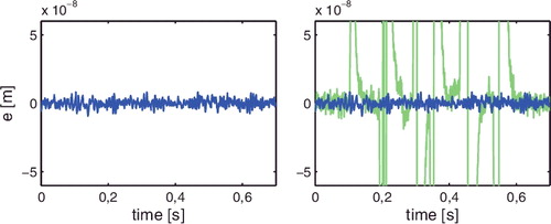
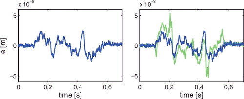
The error $e_{\text{wc}}^1\left(t\right)$ in task j = 1 and cumulative power spectrum are depicted in Figures 7 and 8, respectively. The following observations are made:

Figure 7. Simulation results. The error signal $e_{\mathrm{ wc }}^1(t,{\widehat{\theta }}_{\mathrm{ wc }}^1)$ in task j = 1 shows that $e_{\text{wc}}^1(t,{\widehat{\theta }}_{\mathrm{ wc }}^1)$ contains a significant reference-induced component $e_r^1(t,{\widehat{\theta }}_{\mathrm{ wc }}^1)$ for z₁(t) (left), while $e_{\text{wc}}^1(t,{\widehat{\theta }}_{\mathrm{ wc }}^1)$ is dominated by e¹_w(t) for z_{p, <i >}(t) (right). For comparison, the peak value of the error signal with feedback only is given by 1 × 10⁻⁴ (m).

Figure 8. Simulation results. Cumulative power spectrum of $e_m^1(t,{\bar{\theta }}^1)$ in task j = 1 for $C_{ff}^1(q,{\bar{\theta }}^1)$ (black), and $e_{\text{wc}}^1(t,{\widehat{\theta }}_{\mathrm{ wc }}^1)$ corresponding to $C_{ff}^1(q,{\widehat{\theta }}_{\text{wc}}^1)$ for z₁(t) (red) , z₂(t) (blue) and z_{p, <i >}(t) (green). (To view this figure in colour, please see the online version of the journal.)

(1)	For zp, <i >(t), the contribution of 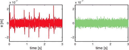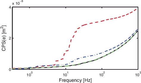$e_r^1(t,{\widehat{\theta }}_{\mathrm{ wc }}^1)$ to $e_{\mathrm{ wc }}^1(t,{\widehat{\theta }}_{\mathrm{ wc }}^1)$ is negligible compared to the contribution of e1w(t). Hence, $e_{\mathrm{ wc }}^1(t,{\widehat{\theta }}_{\mathrm{ wc }}^1)$ is similar to the optimal case $e_m^1(t,{\bar{\theta }}^1)$.
(2)	For z1(t), the contribution of $e_r^1(t,{\widehat{\theta }}_{\mathrm{ wc }}^1)$ to $e_{\mathrm{ wc }}^1(t,{\widehat{\theta }}_{\mathrm{ wc }}^1)$ is significant. As a result, $e_{\mathrm{ wc }}^1(t,{\widehat{\theta }}_{\mathrm{ wc }}^1)$ is significantly degraded compared to the optimal case $e_m^1(t,{\bar{\theta }}^1)$.

Similar results as provided for z₁(t) are obtained for z₂(t), and are omitted for brevity.

The provided simulation study showed that an enhanced accuracy of the parameter estimates results in a reduced difference between $e_{\mathrm{ wc }}^1(t,{\widehat{\theta }}_{\mathrm{ wc }}^1)$ in (36(36) $$\begin{array}{c}\hfill e_{\mathrm{ wc }}^j(t,{\widehat{\theta }}_{\mathrm{ wc }}^j)=e_r^j(t,{\widehat{\theta }}_{\mathrm{ wc }}^j)-e_w^j\left(t\right),\end{array}$$(36) ) and $e_m^1(t,{\bar{\theta }}^1)$ in (35(35) $$\begin{array}{c}\hfill e_m^j(t,{\bar{\theta }}^j)=-e_w^j\left(t\right),\end{array}$$(35) ). Hence, the worst-case error $e_{\text{wc}}^1(t,{\widehat{\theta }}_{\mathrm{ wc }}^1)$ based on a single set of measured data is improved by using the proposed instruments z_{p, <i >}(t). This confirms that the statistical accuracy properties of ${\widehat{\theta }}^j$ are important for performance.

7. Experimental results

In this section, the proposed approach in Section 4 is applied to the prototype industrial nanopositioning system depicted in Figure 9. The positioning stage, measurement system, and actuation system are placed on a vibration isolation table to isolate the system from external disturbances originating from the environment.

Figure 9. Experimental setup with $.5pt-.9pt1$ measurement system, $.5pt-.9pt2$ positioning stage, $.5pt-.9pt3$ linear magnetic actuation system and $.5pt-.9pt4$ vibration isolation table.

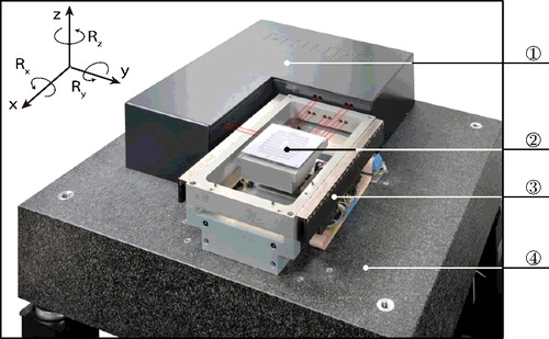
The positioning stage is magnetically levitated and actuated, and controlled in six motion degrees of freedom (DOFs): three translations (x, y, and z) and three rotations (R_x, R_y and R_z). Magnetically levitated stages exhibit contactless operation. Therefore, friction (which is typically an important disturbance in motion control) is eliminated.

The actuation system consists of six linear magnetic motors, with an added position offset such that each actuator can also generate a force in the perpendicular direction. The permanent magnets are connected to the vibration isolation table, while the coils are part of the positioning stage.

The measurement system consists of laser interferometers in conjunction with a mirror block, connected to the vibration isolation table and the positioning stage, respectively. This system enables high-accuracy position measurements in all six motion DOFs. In particular, subnanometer resolution position measurements are available for the translational DOFs x, y and z. Throughout, all systems and signals operate in discrete time with a sampling time of T_s = 2 × 10⁻⁴ s.

7.1 Control configuration and reference signal design

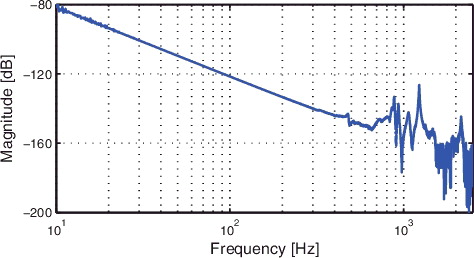
The proposed design procedure for the feedforward controller is applied to the x-direction of the system, i.e. the long-stroke (80 mm) direction of the setup in Figure 9. A stabilising feedback controller $C_{fb}^{\text{mimo}}$ is designed for the multivariable system by means of sequential loopshaping (see Skogestad & Postlethwaite, 2005, Section 10.6) for details. By closing the control loops for the remaining 5 DOFs, i.e. y, z, R_x, R_y and R_z, a single-input, single-output equivalent system P(q) is obtained for the x-direction. The frequency response function of the equivalent system P(q) for the x-direction is depicted in Figure 10. The dynamical response of a linear motion system P(s), where s is the Laplace operator, with proportional damping can be written as a sum of N second-order subsystems (37) $$\begin{array}{c}\hfill \begin{array}{cc}\hfill P\left(s\right)& =\sum _{i=1}^n{\displaystyle \frac{c_i^T{b}_i}{s^2}}+\sum _{i=n+1}^N{\displaystyle \frac{c_i^T{b}_i}{s^2+2{\zeta }_i{\omega }_{i}s+{\omega }_i^2}},\hfill \end{array}\end{array}$$(37) with n the number of rigid-body modes, c^T_i the ith column of the output matrix $C\in {\mathbb{R}}^{n\times N}$, b_i the ith row of the input matrix $B\in {\mathbb{R}}^{N\times n}$, ζ_i the dimensionless damping constant, and ω_i the natural frequency of the ith second-order subsystem. Inspection reveals rigid-body behaviour (as described by the first term in (37(37) $$\begin{array}{c}\hfill \begin{array}{cc}\hfill P\left(s\right)& =\sum _{i=1}^n{\displaystyle \frac{c_i^T{b}_i}{s^2}}+\sum _{i=n+1}^N{\displaystyle \frac{c_i^T{b}_i}{s^2+2{\zeta }_i{\omega }_{i}s+{\omega }_i^2}},\hfill \end{array}\end{array}$$(37) )) below approximately 300 Hz, while the first resonance phenomena (as described by the latter term in (37(37) $$\begin{array}{c}\hfill \begin{array}{cc}\hfill P\left(s\right)& =\sum _{i=1}^n{\displaystyle \frac{c_i^T{b}_i}{s^2}}+\sum _{i=n+1}^N{\displaystyle \frac{c_i^T{b}_i}{s^2+2{\zeta }_i{\omega }_{i}s+{\omega }_i^2}},\hfill \end{array}\end{array}$$(37) )) appear at 480 and 860 Hz. For a motion system with dominant rigid-body dynamics in the frequency range of interest, parametric models are typically developed that only describe the rigid-body dynamics, i.e. the first term in (37(37) $$\begin{array}{c}\hfill \begin{array}{cc}\hfill P\left(s\right)& =\sum _{i=1}^n{\displaystyle \frac{c_i^T{b}_i}{s^2}}+\sum _{i=n+1}^N{\displaystyle \frac{c_i^T{b}_i}{s^2+2{\zeta }_i{\omega }_{i}s+{\omega }_i^2}},\hfill \end{array}\end{array}$$(37) ).

Figure 10. Frequency response function of the considered system P(q) in x-direction.

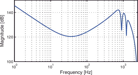
The feedback controller C_fb(q) for the x-direction of the system is depicted in Figure 11, and achieves a bandwidth (defined as the lowest frequency where |C_fbP| = 1) of 120 Hz. This bandwidth results in rejection of low-frequency disturbances, while having sufficient robustness against uncertainty in the resonances of P(q).

Figure 11. Bode diagram of the feedback controller C_fb(q) for the x-direction of the experimental setup.

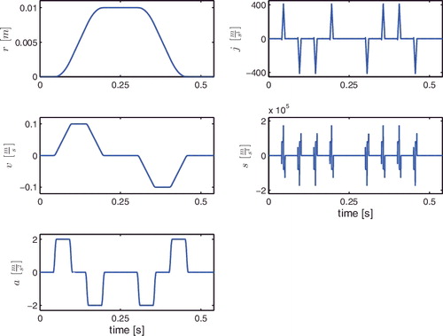
The reference r(t) of the performed servo task is depicted in Figure 12, together with its acceleration, jerk and snap, i.e. the second, third and fourth derivative of r(t).

Figure 12. Position r(t), velocity v(t), jerk j(t), and snap s(t) of the servo task.

7.2 Parametrisation feedforward controller

For the general parametrisation of C_ff(q, θ) in (3(3) $$\begin{array}{cc}\hfill C_{ff}^{j+1}(q,{\theta }^{j+1})& =C_{ff}^j(q,{\theta }^j)+C_{ff}^{\Delta }(q,{\theta }^{\Delta })\hfill \\ & =\sum _{i=1}^{n_{\theta }}{\psi }_i\left(q^{-1}\right)({\theta }_i^j+{\theta }_i^{\Delta }),\hfill \end{array}$$(3) ), (1) the number of parameters n_θ and (2) the selection of basis functions Ψ(q) should be determined to obtain C_ff(q, θ). Here, the parametrisation of C_ff(q, θ) is chosen as in Lambrechts et al. (2005). This parametrisation is developed for motion systems with dominant rigid-body dynamics as in Figure 10, and is given by (38) $$\begin{array}{c}\hfill C_{ff}(q,\theta )=\Psi \left(q\right)\theta ,\end{array}$$(38) with basis functions Ψ(q) = [ψ_v(q⁻¹),  ψ_a(q⁻¹), ψ_j(q⁻¹),  ψ_s(q⁻¹)], where (39) $$\begin{array}{c}\hfill \begin{array}{cc}{\psi }_v\left(q^{-1}\right)=\left({\displaystyle \frac{1-q^{-1}}{T_s}}\right),\hfill & {\psi }_a\left(q^{-1}\right)={\left({\displaystyle \frac{1-q^{-1}}{T_s}}\right)}^2,\hfill \\ {\psi }_j\left(q^{-1}\right)={\left({\displaystyle \frac{1-q^{-1}}{T_s}}\right)}^3,\hfill & {\psi }_s\left(q^{-1}\right)={\left({\displaystyle \frac{1-q^{-1}}{T_s}}\right)}^4,\hfill \end{array}\end{array}$$(39) and corresponding parameters $\theta ={\left[{\theta }_v{\theta }_a{\theta }_j{\theta }_s\right]}^T\in {\mathbb{R}}^{n_{\theta }}$. For C_ff(q, θ) in (40), it holds that $$\begin{array}{c}\hfill C_{ff}{(q,\theta )|}_{q=1}=0,\end{array}$$ i.e. the static gain of C_ff(q, θ) is equal to zero. This condition implies that the feedforward signal u_ff is equal to zero when the system is in stand-still, which is a desired property for motion systems with rigid-body dynamics. Furthermore, recall that the considered experimental setup operates contactless, thereby eliminating performance-deteriorating friction. As such, friction feedforward is not included in the feedforward controller in (40).

7.3 Experimental results for optimal IV method

In this section, the key experimental results of this paper are presented, which involve the application of Procedure 4.1 on the nanopositioning system in Figure 9. Five tasks are performed of N = 2700 samples each, with r(t) as depicted in Figure 12. In addition, r(t) filtered by the basis functions in (41) is shown in Figure 12.

During the jth task, the measured signals e^j_m(t) and y^j_m(t), for t = 1, ..., N, are stored. Then, this batch of measured data is used to determine C^{j + 1}_ff(q, θ^{j + 1}). To initialise Procedure 4.1, C¹_ff(q, θ¹) in the first task has parameters θ¹ = [0,  0,  0,  0]^T, i.e., C¹_ff(q, θ¹) = 0. The performance obtained in task j = 1 is, therefore, the performance with only feedback control applied to the system. Alternatively, the linear least squares estimation approach in van der Meulen et al. (2008) can be used to determine an initial parameter vector θ¹.

The measured error signal e^j_m(t) in the first, second and third task are depicted in Figure 13, while the corresponding cumulative power spectrum is shown in Figure 14. In addition, the two-norm of e^j_m(t), i.e. ‖e^j_m(t)‖₂², as a function of tasks is depicted in Figure 15. The following observations are made:

Figure 13. Experimental results. The measured error signal e^j_m(t) in task j = 1 (red), j = 2 (blue) and j = 3 (green) shows that the peak value of the error signal for feedback only in task j = 1 is 4.5 × 10⁻⁶ (m), and is reduced by 97 % by using iterative feedforward control in j = 3. (To view this figure in colour, please see the online version of this journal.)

Figure 14. Experimental results. Cumulative power spectrum of the measured e^j_m(t) in task j = 1 (red), j = 2 (blue) and j = 3 (green). (To view this figure in colour, please see the online version of this journal.)

Figure 15. The two-norm of the measured error e^j_m(t) as a function of tasks shows convergence in two tasks.

(1)	The peak value of e3m(t) in task j = 3 is reduced by approximately 97% when compared to e1m(t) in the first task. This confirms that the proposed iterative feedforward approach significantly enhances the positioning accuracy of the system compared to only feedback control.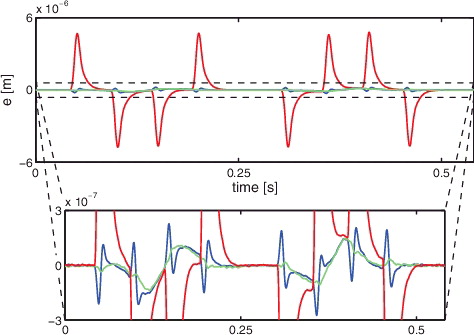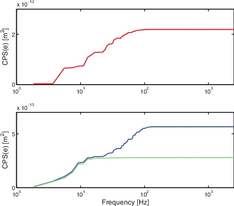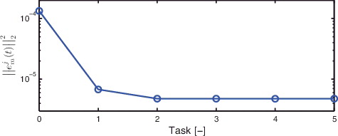
(2)	Figures 13 and 14 show that the low-frequency contribution up to approximately 10 Hz is not compensated for by C3ff(q, θ3) in task j = 3. This implies that the dynamical behaviour of the experimental setup in this frequency range is not captured by the parametrisation proposed in Section 7.2. This can be contributed to the dynamics of the cable connection between the fixed world and the (moving) positioning stage, which acts as a low-frequency disturbance on the system.
(3)	Figure 15 shows that ‖ejm(t)‖22 converges in two tasks. This confirms that fast convergence in terms of ‖ejm(t)‖22 is obtained with the proposed approach.

7.4 Analysis of Algorithm 4.1

The iterative refinement of z_{p, <i >}(t) proposed in Algorithm 4.1 is an essential attribute of Procedure 4.1. In this section, Algorithm 4.1 is illustrated for the considered experimental setup. Recall from (28(28) $$\begin{array}{cc}\hfill z_{\text{opt}}\left(t\right)& =\Psi \left(q\right){(C_{fb}\left(q\right)+C_{ff}^j\left(q\right))}^{-1}{y}_r^j\left(t\right)\hfill \\ & =\Psi \left(q\right){(C_{fb}\left(q\right)+C_{ff}^j\left(q\right))}^{-1}S\left(q\right)P\left(q\right)(C_{fb}\left(q\right)\hfill \\ & +C_{ff}^j\left(q\right))r\left(t\right)\hfill \\ & =\Psi \left(q\right)S\left(q\right)P\left(q\right)r\left(t\right),\hfill \end{array}$$(28) ) that the optimal instruments z_opt(t) can be expressed as $$\begin{array}{c}\hfill z_{\text{opt}}\left(t\right)=\Psi \left(q\right)S\left(q\right)P\left(q\right)r\left(t\right),\end{array}$$ and optimal accuracy is obtained, i.e. z_{p, <i >}(t) = z_opt(t), if $$\begin{array}{c}\hfill {(C_{fb}\left(q\right)+C_{ff,<i>}^j(q,{\widehat{\theta }}_{<i-1>}^{\Delta }))}^{-1}=S\left(q\right)P\left(q\right).\end{array}$$ This result enables a visual illustration of Algorithm 4.1 by comparing the identified frequency response function of S(q)P(q) with the frequency response of (C_fb(q) + C^j_{ff, <i >}(q))^{− 1}.

The analysis in this section is based on the measured signals e¹_m(t) and y¹_m(t), for t = 1, …, N, in task j = 1 with C¹_ff(q, θ¹) implemented on the experimental setup. Furthermore, the number of computational iterations of Algorithm 4.1 is given by K = 3. Figure 16 reveals that (C_fb + C¹_{ff, <3 >})^{− 1} in iteration i = 3 of Algorithm 4.1 is a significantly improved approximation of S(q)P(q) in the frequency range up to 200 Hz, when compared to iteration i = 1. This confirms that iterative refinement of z_{p, <i >}(t) by means of Algorithm 4.1 results in z_{p, <i >}(t) that resemble the optimal z_opt(t).

Figure 16. Iterative refinement of the instruments z_{p, ** < i >}(t) after task j = 1: (C_fb + C¹_{ff, <3 >})^{− 1} (green) corresponding to the i = 3 computational iteration of Algorithm 4.1 is an improved approximation of the frequency response function of the process sensitivity S(q)P(q) (black) compared to (C_fb + C¹_{ff, <1 >})^{− 1} (dashed red) in the i = 1 iteration of Algorithm 4.1. (To view this figure in colour, please see the online version of this journal.)

7.5 Enhanced flexibility to reference variations and comparison with ILC

As is argued in Sections 1 and 2, the key motivation for the proposed feedforward approach compared to ILC algorithms is an enhanced flexibility with respect to changes in the reference trajectory. To demonstrate this flexibility, two similar yet slightly different reference trajectories are applied to the considered nanopositioning system. These reference trajectories are depicted in Figure 17. Then, the optimal IV approach proposed in Section 4 is compared to the standard frequency-domain ILC-based approach (see, e.g. Bristow et al., 2006).

Figure 17. Reference trajectory r₁ for task j = 1, 2, …, 5 (blue) and reference trajectory r₂ for task j = 6, 7, …, 10 (dashed green). (To view this figure in colour, please see the online version of this journal.)

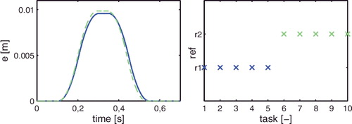
The measured error signals e₅(t) in task j = 5 and e₆(t) in task j = 6 as depicted in Figure 18 for ILC, and in Figure 19 for the proposed optimal IV approach confirm that (1) the servo performance obtained with ILC severely deteriorates when the reference is slightly changed and (2) the proposed approach is insensitive to reference changes. Note that the error in tasks j = 5 is smaller for ILC than for the proposed approach. Since motion systems are typically confronted with similar yet slightly different reference signals (Lambrechts et al., 2005; Oomen et al., 2014), the proposed optimal IV approach is preferred in industrial practice since learning transients are eliminated when the reference trajectory is changed.

Figure 18. Flexibility with respect to changes in the reference trajectory between tasks for ILC. Before task j = 6, the reference trajectory is changed from r₁ to r₂ (see Figure 17). For standard ILC, the measured error signal e₅(t) (blue) in task j = 5 is significantly smaller than for e₆(t) (green) in task j = 6. This confirms that for standard ILC, the servo performance is severely deteriorated if the reference is changed at j = 6. (To view this this figure in colour, please see the online version of this journal.)

Figure 19. Flexibility with respect to changes in the reference trajectory between tasks for the proposed approach in Section 4. Before task j = 6, the reference trajectory is changed from r₁ to r₂ (see Figure 17). The measured error signal e₅(t) (blue) in task j = 5 is similar to e₆(t) (green) in task j = 6, which shows that the servo performance for the proposed IV-approach is invariant to changes in the reference. (To view this figure in colour, please see the online version of this journal.)

8. Conclusions

In this paper, a new algorithm is proposed for iterative feedforward control based on instrumental variables. The key advantage of the proposed algorithm is that it achieves optimal accuracy in terms of variance, in contrast to existing approaches, which are shown to be non-optimal. To achieve optimal accuracy, the proposed algorithm iteratively updates an estimate of the optimal instruments. The assumptions that are introduced in Section 2.2 are for a large class of motion systems nonrestrictive for the achievable performance. If the considered motion system is subject to reference signals with high-frequency signal content, the proposed approach can be extended by allowing more general parametrisations by means of input shaping (Boeren, Bruijnen, van Dijk, et al. 2014) and rational feedforward (Bolder & Oomen, 2015). The proposed method is validated by means of a simulation example, showing improved accuracy compared to pre-existing approaches. Finally, the procedure is successfully applied to an industrial nanopositioning system. The presented experimental results confirm the practical relevance of the proposed approach.

Ongoing research focuses on extensions towards optimal input design (Formentin, Karimi, & Savaresi, 2013a), inferential control, positioning-varying effects (Groot Wassink, van de Wal, Scherer, & Bosgra, 2005) and multivariable systems. For the considered nanopositioning system in Figure 9, improved performance can be obtained by compensating for the dynamics of the cable connection between the fixed world and the (moving) positioning stage by means of feedforward control.

Acknowledgements

The authors acknowledge Maarten Steinbuch and Leon van Breugel for their contribution to this work.

Disclosure statement

No potential conflict of interest was reported by the authors.

Additional information

Funding

This research was supported by Philips Innovation Services and by the Innovational Research Incentives Scheme under the VENI grant Precision Motion: Beyond the Nanometer [grant number 13073] awarded by NWO (The Netherlands Organisation for Scientific Research) and STW (Dutch Science Foundation).

References

- Åström, K. (1970). Introduction to stochastic control theory. Mathematics in science and engineering (Vol. 70). New York, NY: Academic Press.
- Bazanella, A.S., Campestrini, L., & Eckhard, D. (2012). Data-driven controller design: The
- Biagiotti, L., & Melchiorri, C. (2012). FIR filters for online trajectory planning with time- and frequency-domain specifications. Control Engineering Practice, 20, 1385–1399.
- Boeren, F., Blanken, L., Bruijnen, D., & Oomen, T. (2015). Rational iterative feedforward control: Optimal instrumental variable approach for enhanced performance. Proceedings of the conference on decision and control (pp. 6058–6063), Osaka, Japan.
- Boeren, F., Bruijnen, D., & Oomen, T. (2014). Iterative feedforward tuning approach and experimental verification for nano-precision motion systems. Proceedings of the ASME dynamic systems and control conference, San Antonio, TX, USA.
- Boeren, F., Bruijnen, D., van Dijk, N., & Oomen, T. (2014). Joint input shaping and feedforward for point-to-point motion: Automated tuning for an industrial nanopositioning system. IFAC Mechatronics, 24, 572–581.
- Boeren, F., Oomen, T., & Steinbuch, M. (2014). Accuracy aspects in motion feedforward tuning. Proceedings of the American control conference (pp. 2178–2183), Portland, OR, USA.
- Boeren, F., Oomen, T., & Steinbuch, M. (2015). Iterative motion feedforward tuning: A data-driven approach based on instrumental variable identification. Control Engineering Practice, 37, 11–19.
- Boerlage, M., Tousain, R., & Steinbuch, M. (2004). Jerk derivative feedforward control for motion systems. Proceedings of the American control conference (pp. 4843–4848), Boston, MA, USA.
- Bolder, J., & Oomen, T. (2015). Rational basis functions in iterative learning control – with experimental verification on a motion system. IEEE Transactions on Control Systems Technology, 23, 722–729.
- Bristow, D., Tharayil, M., & Alleyne, A. (2006). A survey of iterative learning control: A learning-based method for high-performance tracking control. IEEE Control Systems Magazine, 26, 96–114.
- Butterworth, J., Pao, L., & Abramovitch, D. (2012). Analysis and comparison of three discrete-time feedforward model-inverse control techniques for nonminimum-phase systems. IFAC Mechatronics, 22, 577–587.
- Clayton, G.M., Tien, S., Leang, K.K., Zou, Q., & Devasia, S. (2009). A review of feedforward control approaches in nanopositioning for high-speed SPM. Journal of Dynamic Systems, Measurement, and Control, 131, 0611011–06110119.
- Devasia, S. (2002). Should model-based inverse inputs be used as feedforward under plant uncertainty ? IEEE Transactions on Automatic Control, 47, 1865–1871.
- Fleming, A.J. (2014). Measuring and predicting resolution in nanopositioning systems. IFAC Mechatronics, 24, 605–618.
- Formentin, S., Karimi, A., & Savaresi, S.M. (2013a). Optimal input design for direct data-driven tuning of model-reference controllers. Automatica, 49, 1874–1882.
- Formentin, S., van Heusden, K., & Karimi, A. (2013b). A comparison of model-based and data-driven controller tuning. International Journal of Adaptive Control and Signal Processing, 28, 882–897.
- Forssell, U. (1999). Closed-loop identification: Methods, theory and applications. Linköping: Linköping University.
- Gilson, M., & Van den Hof, P. (2005). Instrumental variable methods for closed-loop system identification. Automatica, 41, 241–249.
- Gorinevsky, D. (2002). Loop-shaping for iterative control of batch processes. IEEE Control Systems Magazine, 22, 55–65.
- Groot Wassink, M., van de Wal, M., Scherer, C., & Bosgra, O. (2005). LPV control for a wafer stage: Beyond the theoretical solution. Control Engineering Practice, 13, 231–245.
- Gunnarsson, S., & Norrlöf, M. (2001). On the design of ILC algorithms using optimization. Automatica, 37, 2011–2016.
- Gunnarsson, S., & Norrlöf, M. (2006). On the disturbance properties of high order iterative learning control algorithms. Automatica, 42, 2031–2034.
- Heertjes, M., Hennekens, D., & Steinbuch, M. (2010). MIMO feed-forward design in wafer scanners using a gradient approximation-based algorithm. Control Engineering Practice, 18, 495–506.
- Hjalmarsson, H. (2009). System identification of complex and structured systems. European Journal of Control, 3, 275–310.
- Hjalmarsson, H., Gevers, M., Gunnarsson, S., & Lequin, O. (1998). Iterative feedback tuning: Theory and applications. IEEE Control Systems, 18, 26–41.
- Hoelzle, D.J., Johnson, A.J.W., & Alleyne, A.G. (2014). Bumpless transfer filter for exogenous feedforward signals. IEEE Transactions on Control Systems Technology, 22, 1581–1588.
- Jakeman, A.J., & Young, P.C. (1979). Refined instrumental variable methods of time-series analysis: Parts II. Multivariable systems. International Journal of Control, 29, 621–644.
- Janot, A., Gautier, M., Jubien, A., & Vandanjon, P.O. (2014). Comparison between the CLOE method and the DIDIM method for robots identification. IEEE Transaction on Control Systems Technology, 22, 1935–1941.
- Janot, A., Vandanjon, P.O., & Gautier, M. (2014a). A generic instrumental variable approach for industrial robot identification. IEEE Transaction on Control Systems Technology, 22, 132–145.
- Janot, A., Vandanjon, P.O., & Gautier, M. (2014b). An instrumental variable approach for rigid industrial robots identification. Control Engineering Practice, 25, 85–101.
- Jung, Y., & Enqvist, M. (2013). Estimating models of inverse systems. Proceedings of the conference on decision and control (pp. 7143–7148), Firenze, Italy.
- Kara-Mohamed, M., Heath, W.P., & Lanzon, A. (2015). Enhanced tracking for nanopositioning systems using feedforward/feedback multivariable control design. IEEE Transactions on Control Systems Technology, 23, 1003–1013.
- Karimi, A., Butcher, M., & Longchamp, R. (2008). Model-free precompensator tuning based on the correlation approach. IEEE Transactions on Control Systems Technology, 16, 1013–1020.
- Khalil, W., & Dombre, E. (2002). Modeling, identification, and control of robots. Bristol, PA: Taylor & Francis.
- Kim, K.S., & Zou, Q. (2013). A modeling-free inversion-based iterative feedforward control for precision output tracking of linear time-invariant systems. IEEE/ASME Transactions on Mechatronics, 18, 1767–1777.
- Kushner, H.J., & Yin, G.G. (2003). Stochastic approximation and recursive algorithms and applications. Stochastic modelling and applied probability (Vol. 35). New York, NY: Springer-Verlag.
- Lambrechts, P., Boerlage, M., & Steinbuch, M. (2005). Trajectory planning and feedforward design for electromechanical motion systems. Control Engineering Practice, 13, 145–157.
- Mishra, S., Coaplen, J., & Tomizuka, M. (2007). Precision positioning of wafer scanners: Segmented iterative learning control for nonrepetitive disturbances. IEEE Control Systems Magazine, 27, 20–25.
- Oomen, T., van Herpen, R., Quist, S., van de Wal, M., Bosgra, O., & Steinbuch, M. (2014). Connecting system identification and robust control for next-generation motion control of a wafer stage. IEEE Transactions on Control Systems Technology, 22, 102–118.
- Puthenpura, S.C., & Sinha, N.K. (1986). Identification of continuous-time systems using instrumental variables with application to an industrial robot. IEEE Transactions on Industrial Electronics, IE-33, 224–229.
- Skogestad, S., & Postlethwaite, I. (2005). Multivariable feedback control: Analysis and design (2nd ed.). West Sussex: John Wiley & Sons.
- Söderström, T. (2002). Discrete-time stochastic systems – estimation and control. London: Springer-Verlag.
- Söderström, T., & Stoica, P. (1983). Instrumental variable methods for system identification. Lecture notes in control and information sciences (Vol. 57). Berlin: Springer-Verlag.
- Söderström, T., & Stoica, P. (1989). System identification. Hemel Hempstead: Prentice Hall.
- Söderström, T., Stoica, P., & Trulsson, E. (1987). Instrumental variable methods for closed loop systems. Proceedings of the IFAC World Congress on automatic control (pp. 363–368), Munich, Germany.
- Steinbuch, M., & Norg, M. (1998). Advanced motion control: An industrial perspective. European Journal of Control, 4, 278–293.
- van de Wal, M., van Baars, G., & Sperling, F. (2000). Reduction of residual vibrations by H∞ feedback control. Proceedings of the fifth motion and vibration conference (MOVIC) (Vol. 2, pp. 481–486), Sydney, Australia.
- van de Wijdeven, J., & Bosgra, O. (2010). Using basis functions in iterative learning control: Analysis and design theory. International Journal of Control, 83, 661–675.
- van der Meulen, S., Tousain, R., & Bosgra, O. (2008). Fixed structure feedforward controller design exploiting iterative trials: Application to a wafer stage and a desktop printer. Journal of Dynamic Systems, Measurement, and Control, 130, 0510061–05100616.
- Yoshida, K., Ikeda, N., & Mayeda, H. (1992). Experimental study of the identification methods for an industrial robot manipulator. Proceedings of the international conference on intelligent robots and systems (pp. 263–270), Raleigh, NC, USA.
- Young, P.C. (1976). Some observations on instrumental variable methods of time-series analysis. International Journal of Control, 23, 293–612.
- Young, P.C. (2015). Refined instrumental variable estimation: Maximum likelihood optimization of a unified Box-Jenkins model. Automatica, 52, 35–46.
- Young, P.C., & Jakeman, A.J. (1979). Refined instrumental variable methods of time-series analysis: Parts I. Single input, single output systems. International Journal of Control, 29, 1–30.
- Young, P.C., & Jakeman, A.J. (1980). Refined instrumental variable methods of time-series analysis: Parts III. Extensions. International Journal of Control, 31, 741–764.
- Zhong, H., Pao, L.Y., & de Callafon, R.A. (2012). Feedforward control for disturbance rejection: Model matching and other methods. Proceedings of the Chinese conference on decision and control (pp. 3525–3533), Taiyuan, China.