The kinematics and static equilibria of a Slinky

Abstract

A Slinky is a loose helical coil spring and is a well-known educational toy. In this paper a model for a Slinky is presented. The Slinky is represented as a sequence of rigid half coils connected by torsional springs. A range of Slinky configurations in static equilibrium are calculated. Where possible the torsion spring model is compared with the much simpler point mass model of a Slinky, and a more sophisticated model that includes axial and shear deformation. The torsional spring model is shown for the most part to produce similar qualitative behaviour as the more complex model. The simplicity of the torsional spring model makes it a candidate for a discrete stair walking dynamic model of a Slinky, The point mass model is straightforward to derive and solve and makes it possible for an undergraduate engineering student in the early part of their degree course to understand. The torsional spring model is a useful tool for showing what can be done in a more advanced mechanics course to model a system that most students would have previous experience of.

KEYWORDS:

• Mechanics
• numerical optimization
• bifurcation
• Slinky

1. Introduction

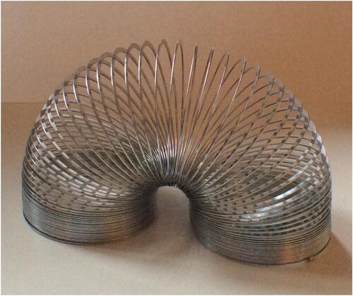
The Slinky is a child’s toy, patented in 1947 (James, 1947). It consists of a flexible helical spring, see Figure 1. Figure 1 shows a Slinky in an arch configuration. A Slinky’s behaviour be it ‘walking’ down some stairs, (Cunningham, 1947) or dropped from a height (Cross & Wheatland, 2012) is mesmerizing and particularly when dropped surprising, when analysed in detail (Graham, 2001). As well as being an educational toy it has also been used to demonstrate physical properties other than the effects of gravity, such as the generation of horizontal and vertical pulses (Blake & Smith, 1979; Gluck, 2010; Vandergrift et al., 1989). The dynamic modelling of Slinkies has for the most part been restricted to approximating the helical spring to a sequence of point masses connected by linear springs. This is a useful model for investigating the dynamics of a dropped spring but cannot be extended to a Slinky descending a stair. One dynamic model for a Slinky descending a stair is a simple two degrees of freedom, two-link model (Hu, 2010). The remaining articles looking at the dynamic behaviour of Slinkies descending stairs are experimental investigations (Cunningham, 1947; Longuet-Higgins, 1954).

Figure 1. Slinky in an arch configuration.

For the modelling of static equilibrium, the point mass model has been applied and some interesting results derived (Eskandari-asl, 2018). For example, for a Slinky fixed at both ends and modelled as a point mass system, the Slinky forms a parabola, and the maximum vertical displacement is independent of the horizontal separation distance between the two fixing points (Eskandari-asl, 2018). As pointed out by Holmes et al. (2014), and considered further below this is a property of the model not the Slinky. Wilson (2001) produced a model for static equilibria of a Slinky by approximating the coils as bars connected by torsional springs. He looked at the arch configuration and the stability of a Slinky. Wilson used his model to predict the number of coils in the arch and the slope angle required for a Slinky to tumble over. Holmes et al. (2014) extended Wilson’s model to include additional springs to account for axial deformation and the effects of shear. Holmes et al. (2014) ultimate intention was to produce a dynamic model, but as yet no model has appeared in the open literature.

The present investigation is one based on a model similar to Wilson’s original model but could ultimately be extended to a dynamic model for analysing a Slinky descending a stair. In this paper attention will be restricted to static equilibria of Slinkies. We will look at the arch configuration as well as other free-end and fixed-end configurations not considered by Wilson (2001). The educational value of analysing a Slinky, be it as a dynamic system or one in static equilibrium, is well known (French, 1994; Gardner, 2000; Gluck, 2010; Graham, 2001; Sawicki, 2002). It is considered here as a window into mechanics for mechanical engineering undergraduate students. The engagement of weaker students in courses in mechanics due to poor mathematical skills is well known and there is a body of knowledge in the literature (Berry et al., 1989; Biggoggero & Rovida, 1977; Graham & Peek, 1997; Graham & Rowlands, 2000), where this problem is analysed and a wealth of solutions presented. For example Cumber (2015) and Widener (2003) present a graphical user interface (GUI) for a pendulum model. A GUI is a software tool that initially shields the student from the mathematics and programming, allowing students to explore parameter space and model behaviour, without getting bogged down in the mathematical detail. Another approach is to present dynamic models that students have some insight into, such as the dynamics of a washing machine (Cumber, 2021). Other papers in this area have looked at how the humble pendulum, often a student’s first experience of a dynamic model has far more interesting behaviour than first imagined (Cumber, 2022; Fay, 2002). This paper is one of a series (Cumber, 2015, 2016, 2017, 2021, 2022) where a simple model is presented that can be derived easily by an undergraduate student and then the analysis of a related more advanced model is presented, making them aware of what is possible in mechanics and the linkages to topics in advanced mechanics.

In this paper a model for static equilibrium of a Slinky is presented. The model is simpler than Holmes et al. (2014), in that it does not consider axial and shear effects. In this respect the model is similar to Wilson (2001) except the helical spring is considered as a series of rigid half coils connected by torsional springs. The analysis of such a model is taken further than Wilson’s investigation. It is also proposed that the simplifications introduced relative to Holmes et al.’s (2014) model in principle can lead to a dynamic model produced by applying the Lagrangian method (Gray et al., 2010) applied to the energy of the system.

2. Point mass model of a Slinky

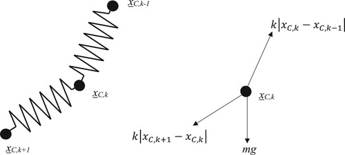
In this representation of a Slinky, the helical coils are represented as point masses connected by linear springs, see Figure 2. The springs are assumed to satisfy Hooke’s law. The free body diagram for a portion of the point mass model is given in Figure 3. Applying a force balance in the x and y directions gives the following system of equations: (1) $\begin{array}{rl}{k}_{\mathrm{pt}}|x_{C,k+1}-x_{C,k}{|}_x& =k_{\mathrm{pt}}|x_{C,k}-x_{C,k-1}{|}_x\\ k_{\mathrm{pt}}|x_{C,k+1}-x_{C,k}{|}_y+\mathrm{mg}& =k_{\mathrm{pt}}|x_{C,k}-x_{C,k-1}{|}_y\\ k& =1,2,\dots ,n\end{array}$(1) The x and y subscripts denote the x and y components of the point vectors. k_pt denotes the spring constant for a linear spring, x_C,k is the location of the kth point mass and m is the mass of a single half coil. The force balance in the x direction leads to the conclusion that the point masses are equi-spaced in the x-direction. The force balance in the y direction can be represented by the linear system $\mathrm{Ay}=b$ where y is the vector of vertical coordinates of the point masses and (2) $A=\left(\begin{array}{cc}\begin{array}{ccc}2& -1& 0\\ -1& 2& -1\\ & & \dots \end{array}& \begin{array}{ccc}& \dots & 0\\ 0& \dots & 0\\ & & \end{array}\\ \begin{array}{ccc}& & \\ 0& & \\ 0& & \end{array}& \begin{array}{ccc}& & \\ 0& 2& -1\\ 0& -1& 2\end{array}\end{array}\right)b=\left(\begin{array}{c}\begin{array}{c}\mathrm{mg}\\ \mathrm{mg}\end{array}\\ \begin{array}{c}\dots \\ \mathrm{mg}\end{array}\end{array}\right)$(2) The solution to the above gives a parabolic curve for the location of the point masses. An interesting point is that the force balance for the vertical components does not depend on the distance between the two fixed ends of the Slinky (Eskandari-asl, 2018). The Slinky model based on rigid half coils and torsional springs for convenience is labelled as the torsional spring model. As we will see below when considering the torsional spring model, this is an artefact of the point mass model not a property of the Slinky. The point mass model is straightforward to formulate but has limited accuracy and the configurations that it can be applied to are limited. It is an excellent starting point for an undergraduate to consider the static equilibrium of a Slinky.

Figure 2. Kinematics of a point mass model for a Slinky.

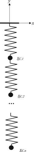
Figure 3. Free body diagram for a point mass model of a Slinky.

3. Torsional spring model of a Slinky

The basic assumption of the torsional spring model is the helical coils are represented as a series of rigid half coils connected by torsional springs. Consider the Slinky arch configuration shown in Figure 1. The maximum distortion of the spring occurs at the edge of the coils on the inside of the arch. This would imply the moment generated by the distortion of the coils on the inside of the arch behaves like a torsional spring. Whether it is large relative to the axial behaviour of the spring is a more open question and will depend on the location and orientation of the fixed ends of the Slinky as well as other physical parameters of the Slinky. The validity of the rigid coil/torsional spring assumption will be considered further below. For the most part we are content to explore the qualitative behaviour of the model. Neglecting shear effects is generally only an issue when the stability of a Slinky is of interest or the end points of the slinky are close together (Holmes et al., 2014).

3.1. Kinematics of the torsional spring model

Initially a slinky fixed at one end will be considered. The starting point is the relationship between the centre of mass of each half coil, x_C,k and the torsion angles ${\theta }_k$, between each pair of half coils, see Figure 4. In Figure 4(a) a number of sequences of angles and point vectors are geometrically defined. The centre of mass of the half coils $\{x_{C,k}{\}}_{k=1}^n$ The end points of the half coils $\{x_{E,k}{\}}_{k=1}^{n+1}$ The torsion angles $\{{\theta }_k{\}}_{k=1}^n$ and the angles the half coils make with the x axis that allows the coordinates of the end points of the half coils to be specified $\{{\phi }_k{\}}_{k=0}^n$

Figure 4. Kinematics of a torsional spring model for a Slinky.

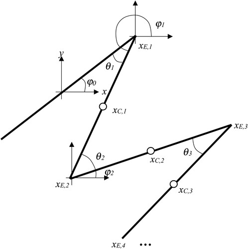
The initial orientation of the surface the Slinky is fixed to is also specified in Figure 4. The slope angle orientation is denoted as ${\phi }_0$. For ${\phi }_0$= 0 the Slinky is orientated to be suspended vertically down. For ${\phi }_0$= 180^o the Slinky is considered to be fixed to the top side of the surface.

An examination of Figure 4 shows that the orientation angles ${\phi }_k$ and torsion angles ${\theta }_k$ are linked. The angle ${\theta }_k$ represents the angle between the half coils labelled as k−1 and k. (3) ${\phi }_k=\left\{\begin{array}{c}{\phi }_{k-1}+{\theta }_k+\pi k\text{is}\text{ odd}\\ {\phi }_{k-1}-{\theta }_k+\pi k\text{is}\text{even}\end{array}\right\}$(3) Defining the sequence (4) ${\mathrm{\Theta }}_k={\phi }_0+\sum _{j=1}^k{\theta }_j(-1{)}^{j+1}$(4) and using the trigonometric addition formulae $\begin{array}{rl}\cos ({\mathrm{\Theta }}_k+\pi )& =-\cos {\mathrm{\Theta }}_k\end{array}$ $\begin{array}{rl}\sin ({\mathrm{\Theta }}_k+\pi )& =-\sin {\mathrm{\Theta }}_k\end{array}$ makes it possible to define the half coil edge point vectors and centre of mass point vectors as (5) $\begin{array}{rl}{x}_{E,k+1}& =x_{E,k}+2R\left(\begin{array}{c}\cos {\mathrm{\Theta }}_k\\ \sin {\mathrm{\Theta }}_k\end{array}\right)(-1{)}^k\end{array}$(5) (6) $\begin{array}{rl}{x}_{C,k+1}& =x_{C,k}+R\left(\begin{array}{c}\cos {\mathrm{\Theta }}_k-\cos {\mathrm{\Theta }}_{k+1}\\ \sin {\mathrm{\Theta }}_k-\sin {\mathrm{\Theta }}_{k+1}\end{array}\right)(-1{)}^k\end{array}$(6) where R is the radius of the Slinky coils, x_C,k is the centre of mass of the kth half coil, and x_E,k is the kth edge as looking at the Slinky from one side. All nomenclature relating to the kinematics of the Slinky is defined in Figure 4. It is possible to simplify (6) further by the application of the trigonometric addition formulae, but the resulting equation is not as useful as (6) in the analysis below. When deriving the energy equation, it is useful to consider the vertical location of the centre of mass of the half coils. Repeated application of (6) gives the following expression for the vertical location of the centres of mass of the half coils. (7) $y_{C,k}=R\left(\sin {\mathrm{\Theta }}_0+2\sum _{j=1}^{k-1}\sin {\mathrm{\Theta }}_j{(-1)}^j+\sin {\mathrm{\Theta }}_k{(-1)}^k\right)$(7)

3.2. Energy equation for a Slinky

We are now in a position to formulate the energy equation for a Slinky. Considering a Slinky with a vertical orientation suspended from a plane with an orientation, ${\phi }_0$, the energy, E, is a summation of the elastic potential energy in the torsional springs and the gravitational potential energy of half coils. (8) $E=\sum _{i=1}^n\frac{1}{2}{k}_r{\theta }_i^2+\sum _{j=1}^n\mathrm{mg}{y}_{C,j}$(8) where k_r is the torsion spring constant. The static equilibria can be found by minimizing the energy (9) $\begin{array}{rl}& \frac{\mathrm{dE}}{d{\theta }_i}=0\\ & k_r{\theta }_i+\mathrm{mg}\sum _{j=1}^n\frac{d{y}_{C,j}}{d{\theta }_i}=0,i=1,2,\dots ,n\\ & \frac{d{y}_{C,j}}{d{\theta }_i}=\left\{\begin{array}{cc}0& i>j\\ -R\text{cos}{\mathrm{\Theta }}_j& i=j\\ R\left(2\sum _{k=i}^{j-1}\cos {\mathrm{\Theta }}_k{(-1)}^{k+i+1}+\cos {\mathrm{\Theta }}_j{(-1)}^{j+i+1}\right)& i<j\end{array}\right\}\end{array}$(9) The above is the system of equations to solve for a Slinky with a vertically down orientation (${\phi }_0$= 0) and fixed at one end only. If the Slinky is fixed at both ends or the initial orientation is above a threshold, then additional physical constraints come into play. For example, the torsion angles cannot be negative and in fact must be above an angle based on the geometry of the Slinky (10) ${\theta }_i\ge {\theta }_{\min }={\tan }^{-1}\left(\frac{\Delta }{2R}\right)$(10) where D is the thickness of a coil. For a Slinky to be fixed at both ends introduce the constraint (11) $x_{E,k}=x_{b,k}\text{for}k=n,n+1$(11) where x_b,k denotes a point vector for the boundary condition imposed on the end half coil of the Slinky. These constraints are accounted for by introducing penalty functions into the energy equation to give the augmented energy. (12) $\begin{array}{rl}{E}_A& =E+P_{{\theta }_{\min }}+P_b\end{array}$(12) (13) $\begin{array}{rl}{P}_{{\theta }_{\min }}& ={\alpha }_{{\theta }_{\min }}\sum _{i=1}^n\{\text{max}(0,-({\theta }_i-{\theta }_{\min })){\}}^2\end{array}$(13) (14) $\begin{array}{rl}{P}_b& ={\alpha }_b\sum _{k=n}^{n+1}(x_{E,k}-x_{b,k}).(x_{E,k}-x_{b,k})\end{array}$(14) ${\alpha }_{{\theta }_{\min }}$ and ${\alpha }_b$ are weightings for the constraints, if these are given too high a value then the numerical optimization process discussed below is more difficult, too low a value and the constraint is not satisfied sufficiently well. The point vectors x_b,n and x_b,n+1 are the boundary conditions for the Slinky. The minimum augmented energy condition is given as (15) $\begin{array}{rl}\frac{d{E}_A}{d{\theta }_i}& =\frac{\mathrm{dE}}{d{\theta }_i}+\frac{d{P}_{{\theta }_{\min }}}{d{\theta }_i}+\frac{d{P}_b}{d{\theta }_i}=0,i=1,2,\dots ,n\end{array}$(15) (16) $\begin{array}{rl}\frac{d{P}_{{\theta }_{\min }}}{d{\theta }_i}& ={\alpha }_{{\theta }_{\min }}\sum _{i=1}^{n}2\{\text{max}(0,-({\theta }_i-{\theta }_{\min }))\}\end{array}$(16) (17) $\begin{array}{rl}\frac{d{P}_b}{d{\theta }_i}& =2{\alpha }_b\sum _{k=n}^{n+1}\left\{{(x_{E,k}-x_{b,k})}_x\frac{d{x}_{E,k,x}}{d{\theta }_i}+{(x_{E,k}-x_{b,k})}_y\frac{d{x}_{E,k,y}}{d{\theta }_i}\right\}\end{array}$(17) where $x_{E,k,x}$ represents the x coordinate of the point vector, x_E,k and $x_{E,k,y}$ represent the y coordinate of the point vector, x_E,k. (18) $\begin{array}{rl}\frac{d{x}_{E,n,x}}{d{\theta }_i}& =2R\sum _{k=i}^{n-1}\sin {\mathrm{\Theta }}_k(-1{)}^{k-i}\end{array}$(18) (19) $\begin{array}{rl}\frac{d{x}_{E,n,y}}{d{\theta }_i}& =2R\sum _{k=i}^{n-1}\cos {\mathrm{\Theta }}_k(-1{)}^{k-i+1}\end{array}$(19)

3.3. Small angle approximate static equilibria

The derivation of an analytic solution of the minimization problem defined by (9) in general is not possible. This leaves the options of looking for approximate solutions that are analytically tractable and numerical optimization algorithms. One approximation technique that is often used in dynamic model analysis is the linearization of the system by making the assumption that the angles in the system are sufficiently small that the approximations for cosine and sine are valid $\begin{array}{rl}\cos {\mathrm{\Theta }}_j& \approx 1\end{array}$ $\begin{array}{rl}\sin {\mathrm{\Theta }}_j& \approx {\mathrm{\Theta }}_j\end{array}$ Making these substitutions in (9) gives the approximate solution (20) ${\theta }_i=\frac{\mathrm{mgR}}{k_r}(n-i+1),i=1,2,\dots ,n$(20) How good a solution this is will be explored in the next section.

3.4. Numerical minimization of energy

The minimizing of the energy requires the solution of the nonlinear system (8) or (12). One method for finding solutions of nonlinear equations is Newton’s method. This method has a second order rate of convergence but requires an initial estimate close to the solution. Unfortunately, the large dimension of the problem makes Newton’s method unsuitable. A further consideration is that as we will discuss later for any given configuration there are multiple solutions. Each solution being a local minimizer of the energy equation (8) or the augmented energy equation (12).

The solution of (9) or (15) is a challenging problem as there are many degrees of freedom depending on the number of coils that make up the Slinky. The two Slinkies considered in the results section below are manufactured from plastic and steel. The parameters for each Slinky are given in Table 1. During the lifetime of this investigation a number of different optimization algorithms have been implemented and applied to the minimization of the energy equation (8) and augmented energy equation (12).

Table 1. Physical parameters of Slinkies.

Material	Nu. Coils	m (g)	R (mm)	L0 (mm)	kr (N/rad)	kpt (N/m)
Plastic	37.5	39	31.5	67	2.572 × 10^−2	26.48
Steel	78.5	192	34	53	0.1582	104.5

The first method implemented is the Nelder Mead method (Nelder & Mead, 1965), sometimes called the Simplex method or the Amoeba method. One of the points in the simplex is the small angle approximation (20). This optimization method is relatively straightforward to implement and does not require the evaluation of the gradient vector $g(\theta )=\left(\begin{array}{c}{k}_r{\theta }_1+\mathrm{mg}\sum _{j=1}^n{\displaystyle \frac{d{y}_{C,j}}{d{\theta }_1}}\\ k_r{\theta }_2+\mathrm{mg}\sum _{j=1}^n{\displaystyle \frac{d{y}_{C,j}}{d{\theta }_2}}\\ \dots \\ k_r{\theta }_n+\mathrm{mg}\sum _{j=1}^n{\displaystyle \frac{d{y}_{C,j}}{d{\theta }_n}}\end{array}\right)$ but tends to work well for low-dimensional spaces only. For the plastic Slinky, see Table 1 for the number of half coils, n = 75. For the Nelder Mead method this is large, but the method does find the minimum energy although it takes many iterations to do so. For the metal Slinky, n = 157, the Nelder Mead method fails to converge.

The second optimization algorithm implemented is the Fletcher–Reeves conjugate gradient method (Fletcher, 1980; Fletcher & Reeves, 1964). This is a guess and correct approach based on solving one-dimensional search problems. The initial guess is the small angle approximate solution (20). This is an optimization method that works well for finding the minimum energy of both the plastic and steel Slinky fixed at one end only. For a Slinky fixed at both ends, the Fletcher–Reeves conjugate gradient method fails to find the minimum augmented energy of the system.

The final optimization method is a quasi-Newton method, the BFGS method (Broyden, 1970a, 1970b; Fletcher, 1980). The quasi-Newton method is a particularly efficient approach that at each iteration generates a search direction based on the gradient vector and an approximation to the Jacobian and in the limit of the iteration count performs in a similar way to Newton’s method. The multiple solution problem, i.e. ensuring that the correct minimizer is found is achieved by starting the problem with ${\alpha }_{{\theta }_{\min }}$ and ${\alpha }_b$ set to zero and then gradually increase these parameters until the boundary condition constraint and minimum angle constraint are satisfied sufficiently accurately.

4. Predictions of static equilibria of a Slinky

In this section the point mass model and the torsion spring model are used to calculate the static equilibria for the plastic and steel Slinky. The main focus is the torsion spring model as it is a more realistic representation of a Slinky and can be applied to more configurations.

4.1. Prediction of a Slinky fixed at one end

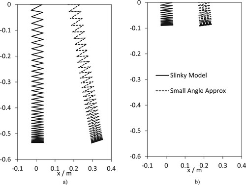
The spring constants k_r and k_pt are calibrated to reproduce the length of the Slinkies in a vertical orientation. For example, the plastic Slinky has a self-weight vertical length of 0.535 m. In Figure 5(a) the plastic Slinky shape is calculated using the torsional spring model satisfying the energy equation (8) and the small angle approximation (20). To make it possible to see the two predictions of the Slinky in Figure 5(a) an origin shift of 0.2 m is applied to the small angle approximation Slinky. The small angle approximation Slinky predicts the correct length but the orientation is incorrect. This is understandable as for coils near the bottom of the Slinky, the small angle approximation is an accurate assumption. At the fixed end near the origin the torsion angles are large due to the self-weight and the small angle approximation is no longer valid. In Figure 5(b) a mini plastic Slinky with 15 coils in a vertical orientation is shown. In this case the small angle approximation works very well.

Figure 5. The plastic Slinky with (a) 37.5 coils and (b) 15 coils.

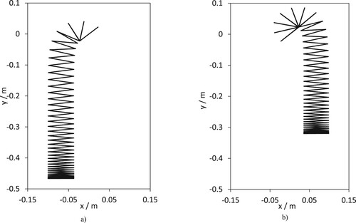
In Figure 6, two static equilibria for the plastic Slinky are shown. The initial orientation of the Slinky is ${\phi }_0$= 135^o. Figure 6(a) shows the static equilibrium of the plastic Slinky calculated by minimizing the energy and the initial estimate of the torsion angles is given by the small angle approximation (20). To calculate the static equilibrium shown in Figure 6(b) the initial estimate in the optimization process is ${\theta }_0=\left(\begin{array}{c}0\\ \pi \\ 0\\ \dots \\ 0\end{array}\right)$ This shows two static equilibria for the same boundary condition, demonstrating that there are multiple static equilibria. In fact, there are many states of static equilibria. To appreciate this, consider the Slinky’s annoying property that it can easily become tangled. There are an almost infinite number of tangled configurations, and each tangled configuration would lead to a local minimum of the energy equation.

Figure 6. Multiple equilibria of a plastic Slinky fixed at one end with an initial orientation of 135^o.

4.2. Prediction of a Slinky fixed at both ends

In this subsection the static equilibrium of a plastic and steel Slinky fixed at both ends is considered. The first configuration considered is a Slinky with an orientation ${\phi }_0$ = 0 and varying the distance between the two end points, D.

In Figure 7 the steel Slinky is shown with ${\phi }_0$= 0, D = 20R and the vertical location of the mid-point of the Slinky, labelled as y_mid is shown with y_mid= −0.28 m. Figure 8(a) shows the functional dependence of y_mid on D for ${\phi }_0$= 0. The graph is made dimensionless with y_mid divided by the radius of the slinky, R, and the separation distance, D, divided by the unstretched length of the Slinky, L₀. Three predictions are shown, the y-coordinate of the mid-point of the Slinky modelled as a series of point masses is a constant line as discussed above, y_mid /R = −4.3. The two other curves are calculated using the torsion spring model, with and without the minimum torsion angle constraint (13) applied. For large spacings, D/L₀ greater than 3, the two predictions are equivalent as the torsion spring angles in static equilibrium are above $\theta$_min and the constraint is not applied. For D/L₀ less than three, the reduced space available for the Slinky coils means that the torsion angles in the midsection of the Slinky are reduced to a point where the $\theta$_min constraint is imposed. The constraint changes the gradient of the curve exhibiting nonlinear behaviour for D/L₀ below 2.

Figure 7. Steel Slinky fixed at either end with ${\phi }_0$= 0, defining D and y_mid.

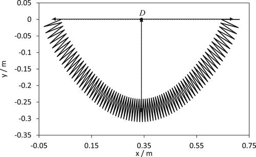
Figure 8. Dimensionless y_mid vs D for ${\phi }_0$ = 0, a) plastic Slinky and b) steel Slinky.

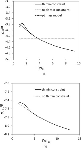
The torsion spring model is more complicated and reflects the kinematics of a Slinky compared to the point mass model. This on its own does not guarantee the torsion spring model is more accurate than the point mass model. Fortunately, Holmes et al. (2014) considered the same configuration for a different Slinky and exactly the same behaviour is demonstrated. Holmes et al.’s (2014) model is more complicated than the torsion spring model as it includes axial and shear deformation effects. Further Holmes et al. (2014) present experimental measurements that follows their models theoretical prediction closely, responding to the $\theta$_min constraint in the same way as the torsion spring model prediction. On this basis it is reasonable to conclude that the torsion spring model is  a more accurate model than the point mass model. The point mass model prediction is located at the approximate average y_mid of the torsion spring model over the range of D/L₀ in the figure. This is encouraging but as demonstrated below is not generally the case. In Figure 8(b) the same predicted D/L₀ vs. y_mid/R curves for the torsion spring model for the metal Slinky are shown. The prediction of y_mid/R of the point mass model, not shown in Figure 8(b), is −10.5, significantly below the torsion spring model curves, for separation distances D/L₀ below 13. The shape of the curves in Figure 8(b) is the same as in Figure 8(a) except the range is −8.1 to −7.4.

The discussion of the following figures extends the configurations to 0^o ≤ ${\phi }_0$ ≤ 180^o for different separation distances. Figure 9 shows the metal Slinky for three symmetric configurations, with ${\phi }_0$= 0^o, 90^o, and 180^o. As expected, the shape of the Slinky in static equilibrium is very different for different orientation angles, ${\phi }_0$. In Figure 9, for all three configurations the separation distance is D = 10R. For small separation distances it is clear that for ${\phi }_0$= 180^o there is reduced space for the Slinky and the configuration changes from a V shaped configuration to an arch. Figure 10 shows y_mid/R vs. D/L₀, calculated using the torsion spring model. The curves for 0^o ≤  ${\phi }_0$ ≤ 90^o have a similar slope to ${\phi }_0$= 0^o with the $\theta$_min constraint (13) growing in significance as the separation distance, D, is reduced. For the ‘up’ configurations, 90^o < ${\phi }_0$ ≤ 180^o the behaviour is similar with the vertical displacement of the midpoint of the Slinky and gradually decreasing with increasing separation distance. For smaller separation distances a saddle-node bifurcation occurs (Holmes et al., 2014) where the configuration changes from a hanging shape to an arch.

Figure 9. A metal Slinky in symmetric configurations with (a) ${\phi }_0$= 0^o, (b) ${\phi }_0$ = 90^o and (c) ${\phi }_0$= 180^o.

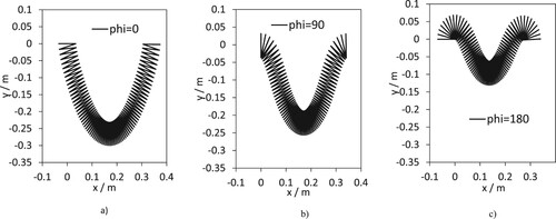
Figure 10. Dimensionless y_mid vs D for a metal Slinky with ${\phi }_0$= 0^o, 60^o, 90^o, 120^o, 150^o, 165^o and 180^o.

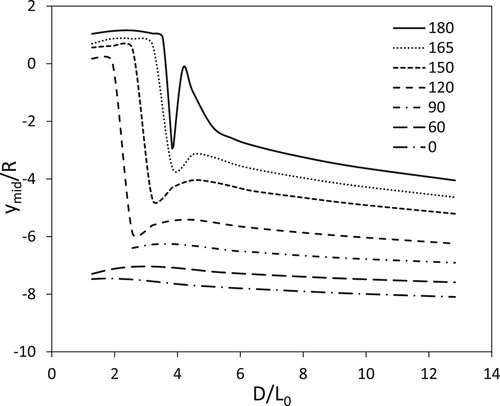
Comparing Figure 10 to the equivalent figure in Holmes et al. (2014), Figure 4, the torsion spring model has the same qualitative behaviour as Holmes et al.’s (2014) model and the experimental measurements for all orientation angles, ${\phi }_0$ except ${\phi }_0$ = 0^o. The difference is the local minimum at D/L₀= 3.85, this is not present in Holmes et al. (2014). The reason for the difference is unclear. One possibility is that the axial deformation and shear deformation effects are important in this part of parameter space. When the fixed ends of a Slinky are close together, the axial deformation of the Slinky is small and is not expected to be important. One interesting point is that D/L₀= 3.85 is equivalent to D = 6R and the separation distance between the edges of the coils is 4R, the space just sufficient for coils to fit side by side. This leads to a hypothesis that neglecting shear deformation is important and the rigidity of coils in the radial direction assumption for this configuration is incorrect. The radial deformation makes it difficult for coils to be aligned side by side and instead the Slinky forms an arch. A second hypothesis is for a given ${\phi }_0$ and D there are multiple states of static equilibrium. Which equilibrium state is realized depends on the path taken in parameter space. Starting with a small value of D and systematically increasing D gives a smooth transition from an arch configuration to a V shaped configuration. Whereas if D is initially large and is systematically reduced then the behaviour of y_mid/R for ${\phi }_0$= 0 follows the shape shown in Figure 10. The path dependency of the static equilibrium realized is called hysteresis. The phenomenon of hysteresis occurs in many areas of physics, chemistry, and engineering. Which hypothesis is correct needs further investigation.

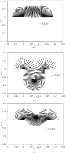
To help appreciation and interpretation of Figure 10 for ${\phi }_0$= 0^o and D/L₀= 3.85, the equivalent of D = 6R, the Slinky static equilibria at D = 5.5R, D = 6R, and D = 6.5R are shown in Figure 11. For D = 5.5R the configuration can be considered arch like in that y_mid is above the base of the Slinky. For D = 6.5R the Slinky forms a V shaped configuration and for D = 6R the configuration is subtlety different forming a U shape.

Figure 11. A metal Slinky in symmetric configurations with ${\phi }_0$ = 180^o, (a) D = 5.5R, (b) D = 6R and(c) D = 6.5R.

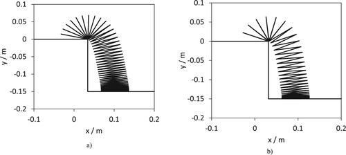
The final Slinky configuration considered is labelled as a ‘stair’ configuration as it is the equivalent of a Slinky with one end on a stair and the other end placed on another stair 0.15 m below. In Figure 12, both the plastic and metal Slinky are shown in the stair configuration. The x coordinate of the centre of the bottom end of the Slinkies are 3R from the centre of the top end of the Slinkies. Both Slinkies look similar to each other apart from the number of coils. The important point is the energy present. The elastic potential energy in both Slinkies is approximately 50% of the total energy present. The metal Slinky has approximately 3.7 times the total energy of the plastic Slinky. The primary interest in this configuration is it provides an initial condition for a dynamic model for a Slinky descending a stair, the starting point for any dynamic model. The torsion spring model captures nearly all the qualitative behaviour Holmes et al. (2014), and is a simpler model.

Figure 12. Slinkies in a stair configuration, (a) metal Slinky and (b) plastic Slinky.

5. Conclusion

In this paper two models of a Slinky are considered, a point mass/linear spring model and a torsion spring model where the Slinky is represented as a series of rigid half coils connected by torsion springs. The torsion spring model is shown to be a more general model than the point mass model as it can be applied to a variety of configurations such as ${\phi }_0$>0^o and the stair configuration. One conclusion of this investigation is the point mass/linear spring theory showing the vertical displacement of the midpoint of a Slinky is independent of the distance between the two fixed end points is a property of the theory rather than the Slinky.

The point mass model still has value as it can be derived using concepts such as force equilibrium, free body diagrams, and Hooke’s law for springs. These concepts are introduced in most introductory undergraduate courses in mechanics. They provide the first steps on the road to more advanced topics in mechanics, such as advanced kinematics, energy conservation, and the Lagrangian method.

The torsion spring model does not include axial and shear deformation, these simplifications are demonstrated to be for the most part second-order effects on the static equilibria of a Slinky. The exception being when the two end points of a Slinky are close together when shear deformation may be important. These simplifications have the potential to provide a route to a dynamic model of a Slinky that more reflects a Slinky’s behaviour than is possible at present using the multiple point mass assumption. This is possible as the route to a dynamic model is to apply the Lagrangian method (Gray et al., 2010) to the expression for the energy of the Slinky (8).

When the torsion spring model could not reproduce the shape of a Slinky i.e. ${\phi }_0$= 180^o and D/L₀= 3.85, two hypotheses are proposed. The shear deformation not included in the torsion spring model is important or the multiple static equilibria come into play and hysteresis determines the actual static equilibria realized. This requires further investigation to identify which hypothesis is correct.

Disclosure statement

No potential conflict of interest was reported by the author.

References

- Berry, J. S., Savage, M., & Williams, J. (1989). Mechanics in decline? International Journal of Mathematical Education in Science and Technology, 20(2), 289–296. https://doi.org/10.1080/0020739890200209
- Biggoggero, G. F., & Rovida, E. (1977). Problems in the teaching of mechanics. European Journal of Engineering Education, 2(4), 277–290. https://doi.org/10.1080/0304379770020406
- Blake, J., & Smith, L. N. (1979). The Slinky as a model for transverse waves in a tenuous plasma. American Journal of Physics, 47(9), 807–808. https://doi.org/10.1119/1.11699
- Broyden, C. G. (1970a). The convergence of a class of double rank minimization algorithms, Part I. IMA Journal of Applied Mathematics, 6(1), 76–90. https://doi.org/10.1093/imamat/6.1.76
- Broyden, C. G. (1970b). The convergence of a class of double rank minimization algorithms, Part II. IMA Journal of Applied Mathematics, 6(3), 222–231. https://doi.org/10.1093/imamat/6.3.222
- Cross, R., & Wheatland, M. S. (2012). Modeling a falling slinky. American Journal of Physics, 80(12), 1051–1060. https://doi.org/10.1119/1.4750489
- Cumber, P. S. (2015). Waggling pendulums and visualisation in mechanics. International Journal of Mathematical Education in Science and Technology, 46(4), 611–630. https://doi.org/10.1080/0020739X.2014.987838
- Cumber, P. S. (2016). Waggling conical pendulums and visualisation in mechanics. International Journal of Mathematical Education in Science and Technology, 47(4), 612–636. https://doi.org/10.1080/0020739X.2015.1088085
- Cumber, P. S. (2017). Visualisation in mechanics: The dynamics of an unbalanced roller. International Journal of Mathematical Education in Science and Technology, 48(3), 434–454. https://doi.org/10.1080/0020739X.2016.1248509
- Cumber, P. S. (2021). Visualisation in mechanics: The dynamics of washing machines. International Journal of Mathematical Education in Science and Technology, 52(4), 626–652. https://doi.org/10.1080/0020739X.2020.1794070
- Cumber, P. S. (2022). There is more than one way to force a pendulum. International Journal of Mathematical Education in Science and Technology, https://doi.org/10.1080/0020739X.2022.2039971
- Cunningham, W. J. (1947). The physics of the tumbling spring. American Journal of Physics, 15(4), 348–352. https://doi.org/10.1119/1.1990962
- Eskandari-asl, A. (2018). Some static properties of Slinky. European Journal of Physics, 39(5), 055005. https://doi.org/10.1088/1361-6404/aacaae
- Fay, T. H. (2002). The pendulum equation. International Journal of Mathematical Education in Science and Technology, 33(4), 505–519. https://doi.org/10.1080/00207390210130868
- Fletcher, R. (1980). Practical methods of optimization, Vol. 1. John Wiley.
- Fletcher, R., & Reeves, C. M. (1964). Function minimization by conjugate gradients. The Computer Journal, 7(2), 149–154. https://doi.org/10.1093/comjnl/7.2.149
- French, A. P. (1994). The suspended Slinky: A problem in static equilibrium. The Physics Teacher, 32(4), 244–245. https://doi.org/10.1119/1.2343983
- Gardner, M. (2000). A slinky problem. The Physics Teacher, 38(2), 78–79. https://doi.org/10.1119/1.1528652
- Gluck, P. (2010). A project on soft springs and the Slinky. Physics Education, 45(2), 178–185. https://doi.org/10.1088/0031-9120/45/2/009
- Graham, E., & Peek, A. (1997). Developing an approach to the introduction of rigid body dynamics. International Journal of Mathematical Education in Science and Technology, 28(3), 373–380. https://doi.org/10.1080/0020739970280307
- Graham, E., & Rowlands, S. (2000). Using computer software in the teaching of mechanics. International Journal of Mathematical Education in Science and Technology, 31(4), 479–493. https://doi.org/10.1080/002073900412598
- Graham, M. (2001). Analysis of Slinky levitation. The Physics Teacher, 39(2), 90–91. https://doi.org/10.1119/1.1355166
- Gray, G. L., Costanzo, F., & Plesha, M. E. (2010). Engineering mechanics dynamics. McGraw Hill.
- Holmes, D. P., Borum, A. D., Moore, W. F., Plaut, R. H., & Dillard, D. A. (2014). Equilibria and instabilities of a Slinky: Discrete model. International Journal of Non-Linear Mechanics, 65, 236–244. https://doi.org/10.1016/j.ijnonlinmec.2014.05.015
- Hu, A.-P. (2010). A simple model of a Slinky walking down stairs. American Journal of Physics, 78(1), 35–39. https://doi.org/10.1119/1.3225921
- James, R. A. (1947). Toy and process of use. U.S. Patent #2415012.
- Longuet-Higgins, M. S. (1954). On Slinky: The dynamics of a loose, heavy spring. Mathematical Proceedings of the Cambridge Philosophical Society, 50(2), 347–351. https://doi.org/10.1017/S030500410002942X
- Nelder, J. A., & Mead, R. (1965). A simplex method for function minimization. The Computer Journal, 7(4), 308–313. https://doi.org/10.1093/comjnl/7.4.308
- Sawicki, M. (2002). Static elongation of a suspended Slinky. The Physics Teacher, 40(5), 276–278. https://doi.org/10.1119/1.1516379
- Vandergrift, G., Baker, T., DiGrazio, J., Dohne, A., Flori, A., Loomis, R., Steel, C., & Velat, D. (1989). Wave cut off on a suspended slinky. American Journal of Physics, 57(10), 949–951. https://doi.org/10.1119/1.15855
- Widener, W. (2003). A graphical user interface for the learning of lateral vehicle dynamics. European Journal of Engineering Education, 28(2), 225–235. https://doi.org/10.1080/0304379031000079059
- Wilson, J. F. (2001). Energy thresholds for tumbling springs. International Journal of Non-Linear Mechanics, 36(8), 1179–1196. https://doi.org/10.1016/S0020-7462(00)00088-3