Error in topographic attributes for volcanic hazard assessment of the Auckland Volcanic Field (New Zealand)

ABSTRACT

Remotely sensed topographic datasets are a major source of information in modelling environmental and geomorphic processes. In this investigation, four of the most popular remotely sensed topographic datasets available for the Auckland Volcanic Field (AVF, New Zealand) were compared using high-accuracy control points, such as real-time kinematic global positioning system (RTK GPS) profiles as well as a terrestrial laser scanning (TLS) surface. The LiDAR (light detection and ranging) data were found to be the most accurate with a root-mean-square error (RMSE) of ±0.9 m, while other datasets such as contour-derived digital elevation model (DEM), Shuttle Radar Topography Mission (SRTM) digital terrain model (DTM) and Advanced Spaceborne Thermal Emission and Reflection Radiometer (ASTER) global DEM (GDEM) were found to be accurate at 5–10 m levels. As part of the error assessment, an extensive comparison was carried out between a range of popular terrain attributes (e.g. elevation, volume and slope angle) to determine their variability as a function of input data properties (e.g. surveying technique and data structure). This study shows that the eruptive volumes of monogenetic volcanoes are sensitive to the input data type and its spatial resolution. The moderately vegetated lava flow fields of Rangitoto have an uncertainty in eruptive volume estimate by ±15% due to the overall surface roughness. For hazard assessment purposes in the AVF, resampled LiDAR datasets are reliable; however, other datasets such as contour-derived DEM and SRTM DTM can be used to estimate eruptive volumes of monogenetic volcanoes.

KEYWORDS:

• ASTER GDEM
• contour DEM
• lava flow
• LiDAR
• root-mean square error
• scoria cone
• slope angle
• SRTM
• topographic survey

Introduction

Spatial data can be stored as discrete measurements such as spot heights, or apparently continuous forms such as digital elevation models (DEMs). The term DEM commonly refers to any type of spatially continuous elevation product, from digitised contour-line-derived DEMs to airborne light detection and ranging (LiDAR) DEMs (e.g. Nelson et al. 2008). The DEMs can be further grouped into digital surface models (DSMs) and digital terrain models (DTMs). The former includes vegetation canopy, buildings and any other anthropogenic feature (e.g. Shuttle Radar Topography Mission data or ‘raw’ unfiltered LiDAR data; e.g. Rabus et al. 2003), whereas the latter contains only ground-surface elevation data (e.g. Liu 2008; Gallay et al. 2013). These DTMs are usually created by post-processing using filtering techniques based on analysis of local (maximum) slope variability (Zhang & Whitman 2005; Meng et al. 2009).

Topographic data created by various techniques (e.g. laser survey, radar, photogrammetry) are used to monitor, model and map environmental and Earth surface processes. These applications can be applied to landslide susceptibility mapping (Kurtz et al. 2014), mass-flow modelling (Procter et al. 2010), drainage network and catchment analysis (Yang et al. 2014), erosion estimations (Kinsey-Henderson & Wilkinson 2013), outcrop modelling (Geyer et al. 2015), vertical fault slip rates (Litchfield et al. 2007), detecting surface ruptures and crustal deformation (Beavan et al. 2012; Villamor et al. 2012), flood inundation modelling (Tarekegn et al. 2010), volcano deformation (Brunori et al. 2013), numerical simulation of lava flows (Del Negro et al. 2013), geomorphic mapping (Liao et al. 2013) and feature extraction and segmentation (Székely et al. 2014). Such modelling studies and mapping of surface features rely on DEMs with various spatial resolutions (Guth 2006; Höhle & Höhle 2009; Chen et al. 2011; Mukherjee et al. 2013). The vertical and horizontal accuracy assessment of digital terrain data have been widely conducted on large continental or country scales using high-accuracy ground control points (Hirt et al. 2010; Shortridge & Messina 2011; Li et al. 2012). Other studies have assessed how these errors ‘inherited’ from digital terrain data affect the results of hazard or susceptibility mapping (Qin et al. 2013), DEM derivatives such as slope angles or drainage networks (Gao 1998; Raaflaub & Collins 2006), or numerical simulations (Huggel et al. 2008).

Applications of such digital topographies for numerical simulations, such as lava flow emplacement (Kereszturi et al. 2014) and susceptibility mapping (Kereszturi et al. 2012), is central to research in the potentially active Auckland Volcanic Field (AVF), New Zealand. This volcanic field coincides with the extent of the largest economic centre in New Zealand, the city of Auckland (Bebbington & Cronin 2011; Agustín-Flores et al. 2015; Spörli et al. 2015). Error ranges of various topographic data sources available for the area of the AVF have not been assessed previously. The aim of this study is therefore to assess the accuracy of topographic datasets available for the AVF, such as LiDAR DTM, Advanced Spaceborne Thermal Emission and Reflection Radiometer (ASTER) GDEM, Shuttle Radar Topography Mission (SRTM) DTM, and a contour-based DTM (Topo50 DEM). The error assessment is based on high-accuracy ground control points surveyed by real-time kinematic global positioning system (RTK GPS) and terrestrial laser scanning (TLS) techniques. This study also aims to assess two topographic derivatives, slope angle and edifice volumes, which are vital input data for volcanic hazard assessments of the AVF (Kereszturi et al. 2012, 2013b) and in volcanic fields elsewhere (Felpeto et al. 2001; El Difrawy et al. 2013; Cappello et al. 2015; Murcia et al. 2015). The error assessment sites were selected to cover a wide range of volcanic morphologies, from the broad cratered maar volcano to a very rough ‘a‘ā lava flow, typical of the AVF.

Materials and methods

Data acquisition and processing of ground control reference datasets

The accuracy of each topographic dataset can be described quantitatively by comparing their terrain elevation to higher-accuracy ground control points/lines or surfaces (Fisher & Tate 2006; Aguilar & Mills 2008; Höhle & Höhle 2009; Wise 2011). In the present study, two different control datasets were used: (1) high-accuracy RTK GPS profiles and (2) a TLS DTM dataset (Figures 1–2).

Figure 1. Overview of topographic data used in this study captured at different spatial scales with different coverage and (vertical) accuracy. Note that the 0.5 m resolution TLS DTM data was used in the present investigation.

The RTK GPS survey data were collected during multiple field campaigns (e.g. Rangitoto, Browns Island and Pukaki volcanoes; Figure 2) using a Leica 1200 RTK GPS. During the surveys, real-time corrections of vertical and horizontal positions were carried out using a base station. The RTK GPS points were surveyed at an accuracy of ≤0.03 m. The dataset consists of topographic profiles with closely spaced measurements (0.5–1 m) over various volcanic terrains such as scoria cones, lava flows and maar craters with different surface coverage (e.g. bare surface and grass-vegetation cover) and geometries. The total number of reference points surveyed was 141 for Rangitoto, 765 for Pukaki and 773 for Browns Island test sites.

Figure 2. High-accuracy reference topographic data from the Auckland region. A, Overview map of the reference data location. Numbered test sites in triangles used in the eruptive volume assessment are: 1, Onepoto; 2, Rangitoto; 3, Browns Island; 4, Panmure Basin; 5, Pukewairiki; 6, Mt Mangere; 7, Mangere Lagoon; 8, Pukeiti and Otuataua; 9, Crater Hill. The rectangles show location of the RTK GPS profiles and TLS surveys. B, RTK GPS profiles from Auckland used in this study. C, Location of the RTK GPS profiles and the TLS survey site on the Rangitoto volcano. On the right hand-side the TLS-based DSM shown here has spatial resolution of 0.5 m.

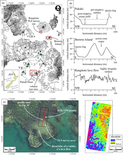
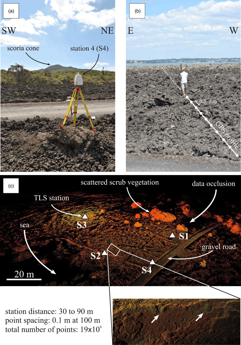
The TLS surveys were carried out using a Leica ScanStation C10 laser scanner (Figures 2–3). This stationary laser scanner has a field of view of 360° horizontally and 270° vertically, with a maximum scanning speed of 50,000 points per second. A TLS survey was carried out on the southernmost part of the Rangitoto Island's ‘a‘ā lava flow units (Figure 3), covering a total in-between survey station area of 90 × 60 m. This test site was chosen due to the absence of substantial vegetation; only individual bushes or grass-type vegetation occurs. The orientation of the scanner was achieved by using backsight points with known coordinate locations. The survey was set up with a vertical and horizontal scanning point density of 10 cm at 100 m from the station points. All point clouds were co-registered using Leica Cyclone 8.0 software. Data filtering, such as outlier filtering, was carried out manually using clipping windows. Outliers included reflections from the sky and minor vegetation, such as grass and scrub (Figure 3). For the whole study area, the point cloud was resampled to 0.1 m average nearest neighbour distances (198.9 × 10³ points).

Figure 3. Field photos of the A, TLS and B, RTK GPS surveys carried out on the distal segment of a rubbly ‘a‘ā lava flow near Flax Point, Rangitoto. C, Perspective view of the TLS point cloud after registration of point from each station. The inset shows the capability of the TLS to resolve detailed features, such as grass (white arrows). Vegetation was removed manually from the point cloud to obtain bare surface points for the DSM.

All surveyed reference data were collected using ellipsoid height (later converted to New Zealand Geodetic Datum 2000 in post-processing) and the New Zealand Transverse Mercator 2000 (NZTM2000) projection.

Data acquisition and processing of topographic datasets

The airborne LiDAR survey data were obtained by Fugro Spatial Solutions and New Zealand Aerial Mapping Limited for Auckland City Council. Two different types of aircraft-mounted LiDAR sensors were used for data capturing. A Leica Airborne Laser Scanner 50 (ALS50) and an Optech Airborne Laser Terrain Mapper 3100-EA (ALTM3100) were used in surveys in 2005–2006 and 2008, respectively. Two types of surveys were carried out in each of these periods, for urban/intertidal and rural areas with different LiDAR settings (for more details see Kereszturi et al. 2012). Post-processing, including filtering and bare-earth point detection of the point cloud, was performed by the data provider, Fugro Spatial Solutions. All point-source data, such as TSL and LiDAR spot heights, were interpolated using the triangulated irregular network (TIN) method. The DTM was created by the data provider (www.fugrospatial.com.au) with a spatial resolution of 2 m. Sinks, flat areas with zero first-derivatives and void removal occur in ≤0.1% of the overall total area. These voids were delimited manually and filled by sink functions implemented into the ILWIS software (ILWIS 2001). This 2 m LiDAR DTM was then resampled into a dataset with 10 m resolution using the nearest neighbour method.

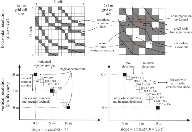
The contour map data of the Auckland area were originally captured by photogrammetry and geodetic surveys, and then later digitised at a scale of 1:50,000. From the vector-based topographic data, only contour lines and shore lines (the 0 m asl contour) were extracted and merged into ArcGIS shape files. Contour lines from the 1:50,000 scale topographic maps were interpolated using a linear interpolation method (Figure 4) implemented into the ILWIS software package (ILWIS 2001). The data processing is described in detail in Kereszturi et al. (2013a). Based on the input data (i.e. contour spacing), a 4 × 4 m grid cell size was chosen because it was small enough to resolve the topography captured by the original contour data. Cell elevation values within a closed contour line are characterised by a flat surface after interpolation (ILWIS 2001). In order to improve the topographic data of the Topo50 DEM, local maxima (n = 39) and minima (n = 7) spot height data were extracted from places with different lithologies (e.g. volcanic deposits, Waitemata Group) from the LiDAR survey. These spot heights were used as control points when new peaks/pits were extrapolated. In the local maxima and minima construction, various DEMs were created with different slope angles from 1° to 15°, based on Jordan (2007). The elevation value at a grid cell location k, within a closed local minimum and maximum contour line, is obtained as:(1) where Z corresponds to the elevation of the last closed contour lines, tanβ is the user-defined degree of slope in the local minima (−) or maxima (+) and d_k is the raster distance between the last contour line and grid cell k. These various local maxima and minima configurations with different slope angles were then compared with the known spot height values obtained from the airborne LiDAR survey. The best fit local minima and maxima DEMs with fewer differences were then chosen to proceed and obtain the final Topo50 DEM.

Figure 4. Structure of data and interpolation from vector-based input data, such as contour lines, using linear interpolation, implemented in the ILWIS software package. Note that there are two examples provided for comparison of the effect of user-defined horizontal resolution and vertical accuracy on the resultant DEM. If the horizontal resolution is set too large (compared to the average distance between two neighbouring contour lines), a flat grid cell is created. If the number of decimals is chosen to be small, then the resultant grid cell elevation might have the same elevation; consequently, a flat grid cell was created.

The space-based DTMs, such as ASTER GDEM version 2 (http://gdem.ersdac.jspacesystems.or.jp/) and SRTM DTM version 4 (Jarvis et al. 2008), were readily available online. Originally, these topographic data used the WGS84 vertical datum (based on the EGM96 geoid) and the WGS84 horizontal projection. To allow for better comparison, in this study both ASTER GDEM (1 arcsecond horizontal resolution, approximately 30 m) and SRTM DTM (3 arcsecond horizontal resolution, approximately 90 m) data were converted into the New Zealand Transverse Mercator 2000 (NZTM2000) projection, while the WGS84 vertical datum was used, assuming a minimal vertical difference (≤0.5 m) between the elliptical-based New Zealand Geodetic Datum 2000 and the WGS84 datum (www.linz.govt.nz). In the re-projection, nearest neighbour resampling was applied.

Benchmarking topographic datasets

Digital terrain model derivatives and their accuracy

There are multiple types of parametric descriptors for terrain morphology (Evans 1972; Speight 1974; Moore et al. 1991; Wood 1996; Shary et al. 2002; MacMillan & Shary 2008; Minár & Evans 2008). In a 3D digital surface, these terrain attributes can be grouped into three categories: zero-order (e.g. elevation), first-order (slope angle) and second-order derivatives (e.g. curvature). In this study, elevation, volume and slope angles along a profile (i.e. in 2D) derived from digital topographies were acquired from various sources and compared with independent, higher-accuracy reference data.

The vertical error of elevation (z) in the digital terrain data can be evaluated by calculating mean error (ME), absolute mean error (|ME|), standard deviation error (S) and root-mean-square error (RMSE) between the topographic data (z_DEM) and the higher-accuracy ground control points (z_control). These error descriptors are defined as (Fisher & Tate 2006):(2) (3) (4) where the total number of control points is n.

Besides the error descriptor, the high-accuracy ground control data were also compared statistically with the elevation derived from the available topographic data from the AVF using linear regression analysis. The equation of the regression lines and goodness-of-fit (R²) are reported.

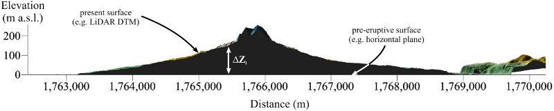
The volumes (V) of a volcanic edifice are very important in volcanic hazard assessment and in reconstructing the eruptive activity of a monogenetic volcanic field (Guilbaud et al. 2012; Kereszturi et al. 2013b). The volume is defined as the enclosed space between the pre-eruptive surface and the present surface (Figure 5). The pre-eruptive surface is usually modelled based on field data and geometric considerations (Kereszturi et al. 2013b). For simplicity, in this study a flat plane was used as a pre-eruptive surface, similar to Kereszturi et al. (2013b). This is justified because the volcanoes from the AVF examined here erupted over a flat alluvial plain (e.g. Manukau Lowlands). The volume between digital surfaces is defined as:(5) where ΔZ_i is the elevation difference between the DSMs/DTMs/DEMs and the pre-eruptive basement at the grid cell location i, with x and y corresponding to the horizontal grid cell dimensions. In total, five scoria cones, five ejecta rings and five lava flows with source scoria cones were used in this study (Figure 1). The example volcanoes were selected based on their volumetric size in order to cover a wide range of volumes in the comparisons. In this assessment, the highest resolution datasets were used (i.e. LiDAR DTM with 2 m spatial resolution) in order to have control data.

Figure 5. Eruptive volume estimation method is shown in the case of Rangitoto volcano.

The gradient vector (G) of a digital surface is characterised by its length, slope angle, as well as its direction, slope aspect (Evans 1972; Zevenbergen & Thorne 1987; Moore et al. 1991; Jordan 2003). Both slope and aspect components are based on numerical differentiation of elevation values around sample location i (e.g. Jordan et al. 2005). It is therefore based on the surrounding grid locations instead of the sample point itself. In 2D, the slope angle is considered here as:(6) where dz and dx are the vertical and horizontal differences around the sample point i.

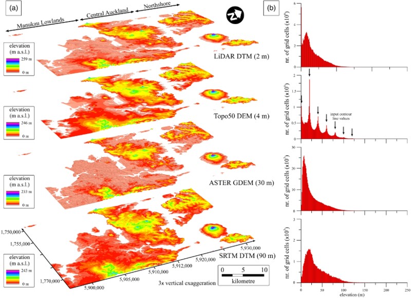
The topographic datasets available in the AVF are presented in Figure 6. Given that Auckland is a coastal city, the choice of a sea-level datum is an additional source of error in data comparisons. The effect of the representation of the sea in different digital topographies was minimised by masking all of the DSM/DTM/DEMs with the same sea level (≤0 m asl) as the LiDAR DTM.

Figure 6. A, Overview of topographic data available in Auckland with various spatial resolutions. From the top to the bottom: 2 m LiDAR DTM, 4 m Topo50 DEM, 30 m ASTER GDEM, 90 m SRTM DTM. B, Elevation histograms.

Results and interpretations

Accuracy of remotely sensed topographic datasets

Description

The error assessment for the available topographic datasets for Auckland was undertaken by comparing these datasets to a finite number of control points surveyed using RTK GPS and TLS techniques (Figure 2). The results of the RMSE calculations and regression analysis are summarised in Tables 1 and 2, respectively.

Table 1. Results of the error assessment of the topographic data for Auckland.

Vertical control data				Topographic datasets
Control data	Location	No. control points	Error descriptor	LiDAR DTM	LiDAR DTM	LiDAR DTM	Topo50 DEM	ASTER GDEM	SRTM DTM
				2 m	10 m	20 m	4 m	30 m	90 m
Profile (RTK GPS)	Browns Island scoria cone	773	RMSE	0.25	0.45	1.30	8.40	No coverage	13.44
			ME	0.02	0.08	0.28	2.45		2.72
			ABS(ME)	0.17	0.31	0.99	7.44		11.44
			S	0.25	0.45	1.27	8.04		13.17
			MIN	−0.88	−1.23	−3.04	−15.21		−26.75
			MAX	2.03	2.22	4.08	13.64		24.87
	Pukaki maar	765	RMSE	1.00	0.15	0.32	11.19	5.74	4.06
			ME	−0.25	−0.05	0.00	8.69	0.10	1.68
			ABS(ME)	0.36	0.09	0.18	10.15	5.05	3.11
			S	0.96	0.14	0.32	7.06	5.74	3.70
			MIN	−4.76	−1.21	−0.59	−6.03	−13.79	−4.61
			MAX	1.11	0.45	1.57	16.29	7.52	13.20
	Rangitoto lava flow	141	RMSE	0.17	0.17	0.20	0.72	1.70	2.26
			ME	0.01	0.01	−0.06	−0.18	−1.50	2.16
			ABS(ME)	0.14	0.14	0.17	0.65	1.56	2.16
			S	0.17	0.17	0.19	0.70	0.79	0.65
			MIN	−0.42	−0.42	−0.54	−1.27	−2.35	0.81
			MAX	0.51	0.54	0.45	1.06	0.80	3.31
Surface (TLS data)	Rangitoto lava flow	57918	RMSE	0.26	0.34	0.36	0.87	2.13	2.44
			ME	−0.06	−0.12	−0.14	0.06	−1.52	2.34
			ABS(ME)	0.20	0.25	0.28	0.77	2.02	0.69
			S	0.25	0.32	0.33	0.71	1.49	2.34
			MIN	−1.18	−1.66	−1.33	−2.14	−3.33	0.86
			MAX	1.19	1.74	1.76	1.98	3.97	4.50

Table 2. Results of the linear regression of the RTK GPS-derived elevation data and the elevation data derived from DSM/DTM and DEMs.

Control data				Topographic dataset
Control data	Location	No. control points	Error descriptor	LiDAR DTM	LiDAR DTM	LiDAR DTM	Topo50 DEM	ASTER GDEM	SRTM DTM
				2 m	10 m	20 m	4 m	30 m	90 m
Profile (RTK GPS)	Browns Island scoria cone	773	slope	0.99	0.98	0.96	0.74	No coverage	0.28
			intercept	0.13	0.38	1.26	9.31		21.61
			R^2	1.000	0.999	0.995	0.745		0.320
	Pukaki maar	765	slope	0.98	0.99	0.99	0.24	0.40	0.74
			intercept	−0.15	−0.04	0.03	14.07	4.38	3.52
			R^2	0.989	1.000	0.999	0.787	0.859	0.855
	Rangitoto lava flow	141	slope	0.29	0.20	0.03	1.52	1.75	1.41
			intercept	1.49	1.69	1.98	−1.28	−3.11	1.28
			R^2	0.249	0.239	0.049	0.157	0.164	0.156

In the Browns Island profile (Figure 7A), the RMSE of the LiDAR dataset including the resampled 10 and 20 m versions is ±0.25, ±0.45 and ±1.30 m (Table 1). The ME and S are 0.016 m and 0.25 m for the 2 m resolution LiDAR DTM, and decrease to 0.28 m and 1.27 m for the resampled LiDAR DTM (20 m version). Other topographic datasets show slightly worse vertical errors, for example the RMSE is ±8.4 m and ±13.4 m for the Topo50 DEM and the SRTM DTM, respectively. The ASTER GDEM has no coverage for Browns Island. The goodness-of-fit (R²) values are extremely high (c. 0.999) for the LiDAR and resampled LiDAR datasets, while R² decreases to 0.744 and 0.319 for the Topo50 DEM and SRTM DTM, respectively (Table 2).

Figure 7. A–C, Profile-based error assessments for the three test sites. The upper row of graphs shows the elevation of different topographic datasets from the AVF. The bottom row of graphs shows the error along the control profile. Note that the Browns Island data have a systematic offset in the original data.

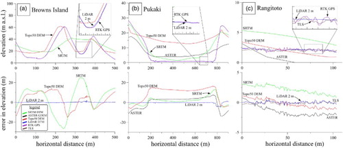
For the Pukaki maar profile (Figure 7B), the accuracy of the LiDAR data is slightly worse than in other profiles (e.g. Browns Island) with a RMSE of ±0.99 m, ME of −0.25 m and S of 0.36 m (Table 1). In the other topographic datasets, the vertical accuracy improved significantly with RMSEs of ±5.73 m and ±4.05 m for the ASTER GDEM and SRTM DTM, respectively; this is in contrast to the Topo50 DEM, where the accuracy decreased to a RMSE of ±11.19 m (Table 1). A similar trend is found with the R² values for the Pukaki maar data (Table 2). However, the performance of the Topo50 DEM, ASTER GDEM and SRTM DTM based on the goodness-of-fit improved to R² values of 0.78–0.86 (Table 2).

The accuracy over the highly rough rubbly ‘a‘ā lava flow on Rangitoto (Figure 7C) shows the smallest deviation from the control RTK GPS profile. All error descriptors are in a very similar range for the LiDAR (e.g. RMSE of ±0.17–0.2 m for both LiDAR and resampled LiDAR DTMs) as it was earlier for other test sites (Table 1). However, the surface representation of the LiDAR DTM was not able to resolve fine-scale (≤2 m) topography (e.g. Figure 8C). The error properties of much coarser datasets are also improved (RMSE of ±0.78 to ±2.25 m), which is in contrast to their visual appearance in representing the ‘true’ surface (Figure 7C). From this site, a TLS DTM-based comparison shows very similar vertical errors, for example the RMSE value is ±0.25 m (Table 1). However, note that the range of elevation values in the TLS DTM is 2.8 m. These low-RMSE values correspond to 28–80% of the elevation values. The overall elevation differences between the TLS DTM reference surface and the examined digital topographies are found to be very narrow (−3.6 to 4.2 m; Table 1), which in turn results in an apparent better overall accuracy in the values for each of the datasets.

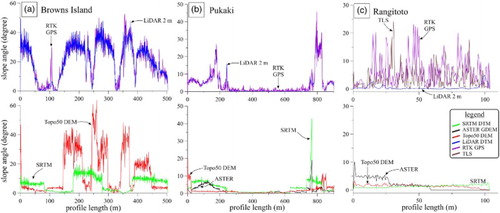
Figure 8. A–C, Error in slope angle derived from profiles from various topographic datasets for the three test sites. For clarity, the upper row of graphs shows LiDAR DTM, RTK GPS and TLS data, while the bottom row of graphs shows Topo50 DEM, ASTER GDEM and SRTM DTM data.

Interpretation

The vertical errors associated with the tested topographic datasets are identical to the often quoted industrial standard values for the vertical and horizontal properties of LiDAR-derived products, ±0.3 to ±0.5 m (e.g. Hodgson & Bresnahan 2004; Gallay 2013). The accuracy, measured along profiles, dropped significantly for both the Topo50 DEM and the remotely sensed SRTM DTM, showing insufficient resolution to resolve the details of the changes of the terrain being modelled. These topographic datasets at Auckland have RMSE values in the range of 5 m (e.g. Topo50 DEM, SRTM DTM) to 10 m (ASTER GDEM). This is consistent with the range of error estimates from different locations (e.g. Gorokhovich & Voustianiouk 2006; Hirt et al. 2010; Shortridge & Messina 2011). On the other hand, the error assessment site on Rangitoto's rubbly ‘a‘ā lava flow showed the smallest deviation (e.g. RMSE values) from the control RTK GPS profile. This result was consistent with the TLS DTM-based error assessment (Table 1). The general topography of Rangitoto at the error assessment site is generally flat with limited or no vegetation cover. In terms of accuracy, this setting for the SRTM and ASTER-derived DTMs is usually associated with an improved RMSE error (e.g. Shortridge & Messina 2011).

This apparently small error of the RMSE descriptor for the LiDAR data is due to the limitation of such parameters in accounting for error on multiple spatial scales. Similar limitations of the RMSE are noted earlier, such as the non-normal distribution of error and non-homogenous spatial distribution of ground control points (e.g. Wise 2011; Zandbergen 2011). For instance, in the case of the LiDAR-based profile (e.g. Figure 7C), the profile accurately represents the surface on a metre-scale and it obviously fails to account for millimetre to decimetre spatial scales.

This scale-dependence of the error descriptor should be investigated in terms of its impact on various applications in the AVF, such as numerical lava flow simulations or watershed mapping. The accuracy of these datasets implies that anything that is smaller than this vertical error (e.g. c. 1 m; Table 1) is represented in the digital topographies with a high uncertainty. For instance, this vertical error might affect lava flow simulation results, in which the simulated lava flow thicknesses are often in a similar range such as mean thicknesses of 3.5 m for Little Rangitoto, 6.1 m for Mt Roskill and 11.4 m for Three Kings (Kereszturi et al. 2014). The maximum error range is equivalent to 28.5%, 16.4% and 8.8% of the thicknesses of the lava flows listed above. The accuracy of simulation results beyond these values is therefore hampered by the high level of uncertainty in the topographic data used.

Accuracy of slope angles along profiles

Description

In this study, slope angles were calculated along each RTK GPS profile (Figure 8). For each case, the data were compared statistically with the higher-accuracy control points from the RTK GPS profiles. The measure of how close the data fit to the reference data, described here with R² values, shows a gradual decrease towards the coarse resolution datasets such as Topo50 DEM, ASTER GDEM and SRTM DTM (Table 3). The best fit was found for the topographic derivatives from the LiDAR and resampled LiDAR datasets (R² of 0.75–0.90; Table 3). However, these data do not match as well as the elevation data. Departures from the reference profile in the case of the Topo50 DEM, SRTM DTM and ASTER GDEM datasets are also visible in the profiles (Figure 8). The poor fit for the very rough ‘a‘ā lava flow surface is also apparent (Table 3).

Table 3. Results of the linear regression of the RTK GPS-based slope angle and the slope angles from DSM/DTM and DEMs.

Control data				Topographic dataset
Control data	Location	No. control points	Error descriptor	LiDAR DTM	LiDAR DTM	LiDAR DTM	Topo50 DEM	ASTER GDEM	SRTM DTM
				2 m	10 m	20 m	4 m	30 m	90 m
Profile (RTK GPS)	Browns Island scoria cone	773	slope	0.93	0.90	0.86	0.60	No coverage	0.08
			intercept	0.98	1.27	1.17	1.44		4.77
			R^2	0.883	0.832	0.746	0.263		0.047
	Pukaki maar	765	slope	0.84	0.88	0.90	0.07	0.11	0.21
			intercept	0.36	0.03	−0.11	1.31	0.98	2.01
			R^2	0.706	0.838	0.891	0.052	0.177	0.250
	Rangitoto lava flow	141	slope	−0.005	−0.009	−0.11	0.012	−0.01	0.006
			intercept	0.53	0.33	1.35	1.31	1.78	1.31
			R^2	0.001	0.039	0.011	0.014	0.001	0.006

Interpretation

The slope angles calculated in 2D from RTK GPS profiles match with the derivatives from the airborne LiDAR DTM and the resampled DTM values. The slightly worse linear regression fitting data suggests that the derivatives enhance error originated from the elevation values (e.g. Jordan 2007). This might be associated in the original elevation values with terrain steepness (i.e. the steeper the terrain, the larger the error related to the elevation values) and changes in vegetation cover type (e.g. low grass and high grass cover). This has been documented previously for LiDAR-derived datasets (e.g. Hodgson et al. 2005). The resampling did not introduce any significant modification to the terrain derivatives, such as slope angles (e.g. Figure 8). This is further supported by RMSE values of the resampled LiDAR dataset (e.g. Table 1). Interestingly, there is a slight improvement of the fitting of the slope angle derivatives against the reference data after resampling to a coarser resolution (e.g. 10 and 20 m LiDAR DTM at the Pukaki site; Table 3). Besides this anomaly, the trends are consistent with other studies (e.g. Wu et al. 2008).

Accuracy of volume estimates from digital terrain models

Description

In this study, three morphologically and genetically different parts of a monogenetic volcano were considered, including ejecta rings, scoria cones and scoria cones with lava flows (Tables S1–S3).¹ The results show that the differences in volumes calculated from resampled datasets are very steady (Figure 9). The resampling of the LiDAR DTM data introduced differences as large as ±3.2% for ejecta rings, ±4.8% for scoria cones and ±4.3% for lava flows (Tables S1–S3).

Figure 9. Error in eruptive volume estimations due to resampling and different input data types, including LiDAR DSM 2 m (triangle), Topo50 DEM (diamond), ASTER GDEM (circle) and SRTM DTM (rectangle). This graph shows the overall inaccuracy of ASTER and SRTM DTM products in resolving the fine-scaled details of the topography on monogenetic volcanoes.

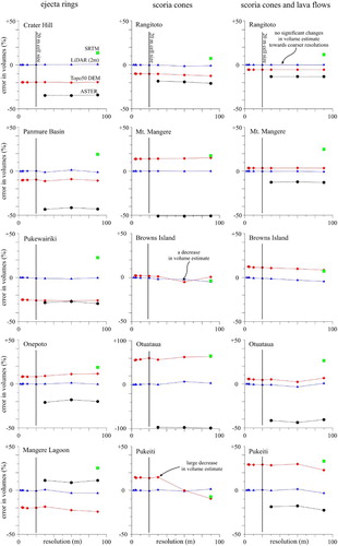
There are large differences in the volumes estimated from topographic datasets surveyed with different techniques and at different original sampling intervals (Figure 9). Comparing volume estimates with the high-resolution LiDAR DTM as the reference data, the Topo50 DEM usually under- and overestimates the volumes by 20% for ejecta rings and lava flows. The largest difference was for one of the smallest volcanic edifices of the AVF, the Otuataua scoria cone, the volume of which was overestimated by as much as 63% (Tables S1–S3). The remotely sensed DTM, such as the SRTM, performed surprisingly in a very similar range (±20%) to the Topo50 DEM. The worst volume estimates were obtained from the ASTER GDEM, which under- or overestimated the data by 90% (e.g. Otuataua scoria cone; Tables S1–S3).

Interpretation

The volumes of the volcanic components of volcanic fields are essential for estimating the temporal and spatial magma flux (e.g. Kereszturi et al. 2013b). The error associated with Topo50 DEM and SRTM DTM datasets estimated here is interpreted as demonstrating they are a reliable source of volume estimates for monogenetic volcanoes. On the other hand, the volume calculation results from the ASTER GDEM show that this source of data is not good enough for extremely small edifices (i.e. 200–300 m in diameter) such as Otuataua (up to 95% difference). The dimensions of larger landforms (i.e. ≥300 m in diameter) are found to be well estimated within a difference range of ±20–30%. This is consistent with the volume calculation of sand dunes (Grohmann & Sawakuchi 2013) and monogenetic volcanoes (Fornaciai et al. 2012) reported elsewhere.

Terrestrial laser scanning

Description

Using the TLS DTM, the examined DSM/DTM/DEM failed to resolve the fine-scale (≤1 m) details of the terrain at the Rangitoto site. The elevation difference maps and distribution show a wide scatter (Figure 10). For the LiDAR DTM, the elevation difference shows a symmetric distribution with a mean of −0.06 m. The rest of the topographic datasets show multi-modal distributions (Figure 10). On closer view (Figure 11), the systematic under- and overestimation of the topography by the airborne LiDAR DTM is shown.

Figure 10. Surface-based error assessment based on a TLS acquired reference surface on the distal part of the Rangitoto lava flow field. Note the multimodal error distributions for the Topo50 DEM, ASTER GDEM and SRTM DTMs. These are due to the dominance of under- and overestimation of the real topography.

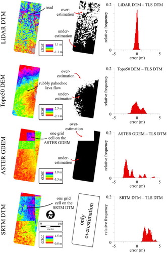
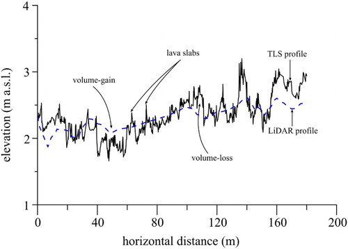
Figure 11. Surface roughness at centimetre–millimetre scales shown using the TLS data (black line) on the distal parts of Rangitoto ‘a‘ā lava flow with respect to the LiDAR profile (dashed line).

Even though the spatial extent of the TLS DTM is limited to an area of 100 × 200 m (Figure 10), it can be used to assess the degree of information loss due to under-representation of the fine-scale features of the topography. Here, the volume between the TLS DTM and an arbitrary plane at sea level was calculated. This returned a volume of 3.7 × 10⁴ m³ (Table 4). By comparison, the LiDAR DTM and Topo50 DEM returned 83–91% of this volume, while the ASTER GDEM and SRTM DTM seriously over- and underestimated the total volume by 70% and 78%, respectively (Table 4).

Table 4. Results of volume estimates based on the TLS data and the percentage error of volumes estimated from other topographic datasets in the AVF.

Dataset	Resolution (m)	Volume (10^4 m^3)	Percentage (%)
TLS DTM	0.5	3.76400	100.0
LiDAR DTM	2	3.22864	85.8
LiDAR 10 m DTM	10	3.13705	83.3
LiDAR 20 m DTM	20	3.11638	82.8
Topo50 DEM	4	3.41133	90.6
ASTER GDEM	30	1.11154	29.5
SRTM DTM	90	6.71175	178.3

Interpretation

This loss of the fine-scaled details of the topography is an issue for Rangitoto Island only in the AVF. The inaccuracy of any topographic data in resolving the fine details of the topography (e.g. Figures 10–11) has an important implication in the calculation of eruptive volumes. Based on the estimated range of differences between the reference TLS data and the available topographic data, Rangitoto's bulk volume, which has been calculated before to be 1.083 km³ (Kereszturi et al. 2013b), can change by as much as ±15% due to the insufficient terrain representation in the 2 m resolution LiDAR DTM in the AVF. The LiDAR data and its resampled products over Rangitoto therefore do not resolve the topography, but they tend to smooth the terrain being modelled at sub-metre scale (Figure 11). This smoothing is due to the insufficient point density or sampling intervals used in the LiDAR surveys. Other older volcanoes of the AVF (e.g. Lindsay et al. 2011) have much smoother surfaces due to soil cover and weathering products; this issue therefore does not affect their estimated volumes. Consequently, these volcanic edifices are expected to be well characterised by the resampled DSM topographic datasets.

This loss of the fine-scaled details of the topography can also influence the surface roughness. The surface roughness is often found to have a strong correlation with the time elapsed since the emplacement of the lava flow (e.g. Farr 1992) or with the overall grain size distribution of the deposits (e.g. Mazzarini et al. 2008). In further examining of the LiDAR DTM of the extremely rough lava flow surface of Rangitoto (Figure 11), it is evident that the surface roughness of bare lava flows is the largest contributor to the overall uncertainty in the volume estimates. This variation in roughness is present on metre–millimetre scales (e.g. Farr 1992; Shepard et al. 2001), as captured by the TLS DTM in comparisons with the LiDAR (Figure 11).

Conclusions

Based on the relative and absolute accuracy of each topographic dataset available for the Auckland region, the best performance ranking is (in decreasing order): the LiDAR DTM, Topo50 DEM, SRTM DTM and ASTER GDEM (Table 1). The LiDAR DTM has a RMSE of ±0.28 m, which is comparable to other LiDAR-based studies (e.g. Hodgson & Bresnahan 2004; Aguilar & Mills 2008). This is in agreement with the performance of the terrain attributes and their changes as a function of horizontal grid cell size. For the purpose of volcanic hazard assessment in the AVF, the LiDAR dataset and its resampled derivatives (e.g. 10 and 20 m) should be preferred.

This calibration of terrain data available for the Auckland region, and the accuracy of extractable terrain attributes, is important for establishing the overall limits of the input data in terms of terrain representation. Furthermore, the appropriate ‘scale’ of the subsequent investigation also needs to be determined based on available topographic data. The working scale (i.e. resolution) for our calculations is between 5 and 10 m, and occasionally less detailed topographic data are acceptable (i.e. ≤20 m). This is consistent with the suggested working resolution for any hydrological and geomorphic mapping studies and landform/feature extraction found elsewhere (e.g. Zhang & Montgomery 1994). For any subsequent investigations in the AVF it will therefore be appropriate and acceptable to extract quantitative topographic information, such as eruptive volumes, using a subset of the resampled LiDAR DTM data.

Surface roughness of lava flows and any other volcanic terrains is an important contributor to the inaccurate representation of a digital terrain acquired by most of the available DSM/DTM and DEM worldwide. This limitation, due to the extreme variability of surface roughness on volcanic terrain, has to be quantified and assessed before estimation of volumes can be determined. In Auckland, the largest uncertainty associated with surface roughness is observed at Rangitoto, while all other volcanoes are characterised by much smoother surfaces due to weathering and erosion over the last few thousand years.

In future research, surface roughness and its relation to the digital terrain representation should be investigated in order to reveal ‘optimal’ resolutions required to assess and model various environmental processes such as modelling lava flow emplacement by numerical models or volcanic hazard mapping.

Supplementary data

Table S1. Summary of volume changes of ejecta rings due to different grid cell size for all datasets of the AVF. The volumes are reported in cubic metres.

Table S2. Summary of volume changes of lava flows with source scoria cones due to different grid cell size for all datasets of the AVF. The volumes are reported in cubic metres.

Table S3. Summary of volume changes of scoria cones due to different grid cell size for all datasets of the AVF. The volumes are reported in cubic metres.

Acknowledgements

The manuscript for this article benefitted from critical reviews by Gyozo Jordan, Kate Arentsen, Shane Cronin and Károly Nemeth. During the GPS survey and TLS surveys the important help from Bruce Robinson and Simon Smith at Global Survey (www.globalsurvey.co.nz) is appreciated. The authors are thankful for the constructive review by Salman Ashraf, an anonymous reviewer, and the journal’s Associate Editor, Andrew Gorman.

Associate Editor: Associate Professor Andrew Gorman.

Disclosure statement

No potential conflict of interest was reported by the authors.

ORCID

G Kereszturi http://orcid.org/0000-0003-4336-2012

Additional information

Funding

GK thanks the Institute of Agriculture and Environment at Massey University (New Zealand) for a PhD Research Scholarship. This work was supported by the FRST-IIOF project ‘Facing the challenge of Auckland's volcanism’, as well as the New Zealand Natural Hazards Research Platform project ‘Living with Volcanic Risk’. We also gratefully acknowledge funding support from Jan Lindsay and the DEtermining VOlcanic Risk in Auckland (DEVORA) project co-funded by the NZ Earthquake Commission (EQC) and the Auckland City Council.

References

- Aguilar FJ, Mills JP. 2008. Accuracy assessment of LiDAR-derived digital elevation models. The Photogrammetric Record. 23:148–169. doi: 10.1111/j.1477-9730.2008.00476.x
- Agustín-Flores J, Németh K, Cronin S, Lindsay J, Kereszturi G. 2015. Construction of the North Head (Maungauika) tuff cone: a product of Surtseyan volcanism, rare in the Auckland Volcanic Field, New Zealand. B Volcanol. 77:1–17. doi: 10.1007/s00445-014-0892-9
- Beavan J, Motagh M, Fielding EJ, Donnelly N, Collett D. 2012. Fault slip models of the 2010–2011 Canterbury, New Zealand, earthquakes from geodetic data and observations of postseismic ground deformation. New Zeal J Geol Geophys. 55:207–221. doi: 10.1080/00288306.2012.697472
- Bebbington MS, Cronin SJ. 2011. Spatio-temporal hazard estimation in the Auckland Volcanic Field, New Zealand, with a new event-order model. B Volcanol. 73:55–72. doi: 10.1007/s00445-010-0403-6
- Brunori CA, Bignami C, Stramondo S, Bustos E. 2013. 20 years of active deformation on volcano caldera: joint analysis of InSAR and AInSAR techniques. Int J Appl Earth Obs. 23:279–287. doi: 10.1016/j.jag.2012.10.003
- Cappello A, Zanon V, Del Negro C, Ferreira TJL, Queiroz MGPS. 2015. Exploring lava-flow hazards at Pico Island, Azores Archipelago (Portugal). Terra Nova. 27:156–161. doi: 10.1111/ter.12143
- Chen C-F, Fan Z-M, Yue T-X, Dai H-L. 2011. A robust estimator for the accuracy assessment of remote-sensing-derived DEMs. Int J Remote Sens. 33:2482–2497. doi: 10.1080/01431161.2011.615766
- Del Negro C, Cappello A, Neri M, Bilotta G, Herault A, Ganci G. 2013. Lava flow hazards at Mount Etna: constraints imposed by eruptive history and numerical simulations. Sci. Rep. 3, article no. 3493. doi:10.1038/srep03493.
- El Difrawy MA, Runge MG, Moufti MR, Cronin SJ, Bebbington M. 2013. A first hazard analysis of the Quaternary Harrat Al-Madinah volcanic field, Saudi Arabia. J Volcanol Geoth Res. 267:39–46. doi: 10.1016/j.jvolgeores.2013.09.006
- Evans IS. 1972. General geomorphometry, derivatives of altitude and descriptive statistics. In: Chorley RJ, editor. Spatial analysis in geomorphology. London: Methuen; p. 17–90.
- Farr TG. 1992. Microtopographic evolution of lava flows at Cima Volcanic Field, Mojave Desert, California. J Geophys Res: Solid Earth. 97:15171–15179. doi: 10.1029/92JB01592
- Felpeto A, Araña V, Ortiz R, Astiz M, García A. 2001. Assessment and modelling of lava flow hazard on Lanzarote (Canary Islands). Nat Hazards. 23:247–257. doi: 10.1023/A:1011112330766
- Fisher PF, Tate NJ. 2006. Causes and consequences of error in digital elevation models. Prog Phys Geog. 30:467–489. doi: 10.1191/0309133306pp492ra
- Fornaciai A, Favalli M, Karátson D, Tarquini S, Boschi E. 2012. Morphometry of scoria cones, and their relation to geodynamic setting: a DEM-based analysis. J Volcanol Geoth Res. 217–218:56–72. doi: 10.1016/j.jvolgeores.2011.12.012
- Gallay M. 2013. Direct acquisition of data: airborne laser scanning. Geomorphological Techniques. 2:1–17.
- Gallay M, Lloyd CD, McKinley J, Barry L. 2013. Assessing modern ground survey methods and airborne laser scanning for digital terrain modelling: a case study from the Lake District, England. Comput Geosci. 51:216–227. doi: 10.1016/j.cageo.2012.08.015
- Gao J. 1998. Impact of sampling intervals on the reliability of topographic variables mapped from grid DEMs at a micro-scale. Int J Geogr Inf Sci. 12:875–890. doi: 10.1080/136588198241545
- Geyer A, García-Sellés D, Pedrazzi D, Barde-Cabusson S, Marti J, Muñoz JA. 2015. Studying monogenetic volcanoes with a terrestrial laser scanner: case study at Croscat volcano (Garrotxa Volcanic Field, Spain). B Volcanol. 77:1–14. doi: 10.1007/s00445-015-0909-z
- Gorokhovich Y, Voustianiouk A. 2006. Accuracy assessment of the processed SRTM-based elevation data by CGIAR using field data from USA and Thailand and its relation to the terrain characteristics. Remote Sens Environ. 104:409–415. doi: 10.1016/j.rse.2006.05.012
- Grohmann CH, Sawakuchi AO. 2013. Influence of cell size on volume calculation using digital terrain models: a case of coastal dune fields. Geomorphology. 180–181:130–136. doi: 10.1016/j.geomorph.2012.09.012
- Guilbaud M-N, Siebe C, Layer P, Salinas S. 2012. Reconstruction of the volcanic history of the Tacámbaro-Puruarán area (Michoacán, México) reveals high frequency of Holocene monogenetic eruptions. B Volcanol. 74:1187–1211. doi: 10.1007/s00445-012-0594-0
- Guth PL. 2006. Geomorphometry from SRTM: Comparison to NED. Photogramm Eng Rem S. 72:269–277. doi: 10.14358/PERS.72.3.269
- Hirt C, Filmer MS, Featherstone WE. 2010. Comparison and validation of the recent freely available ASTER-GDEM ver1, SRTM ver4.1 and GEODATA DEM-9S ver3 digital elevation models over Australia. Aust J Earth Sci. 57:337–347. doi: 10.1080/08120091003677553
- Hodgson ME, Bresnahan P. 2004. Accuracy of airborne Lidar-derived elevation: empirical assessment and error budget. Photogramm Eng Rem Sens. 70:331–339. doi: 10.14358/PERS.70.3.331
- Hodgson ME, Jensen J, Raber G, Tullis J, Davis BA, Thompson G, Schuckman K. 2005. An elevation of LiDAR-derived elevation and terrain slope in leaf-off conditions. Photogramm Eng Rem Sens. 71:817–823. doi: 10.14358/PERS.71.7.817
- Höhle J, Höhle M. 2009. Accuracy assessment of digital elevation models by means of robust statistical methods. ISPRS J Photogramm. 64:398–406. doi: 10.1016/j.isprsjprs.2009.02.003
- Huggel C, Schneider D, Miranda PJ, Delgado Granados H, Kääb A. 2008. Evaluation of ASTER and SRTM DEM data for lahar modeling: a case study on lahars from Popocatépetl Volcano, Mexico. J Volcanol Geoth Res. 170:99–110. doi: 10.1016/j.jvolgeores.2007.09.005
- ILWIS. 2001. ILWIS 3.0 Academic—user’s guide [Internet]. Enschede, The Netherlands: Unit Geo Software Development Sector Remote Sensing and GIS IT Department, International Institute for Aerospace Survey and Earth Sciences (ITC); [cited 2016 May 17]. Available from: http://www.itc.nl/ilwis/documentation/version3.asp
- Jarvis A, Reuter HI, Nelson A, Guevara E. 2008. Hole-filled SRTM for the globe. Version 4 [Internet]. CGIAR-CSI SRTM 90m Database. [cited 2016 May 17]. Available from: http://www.cgiar-csi.org/data/srtm-90m-digital-elevation-database-v4-1
- Jordan G. 2003. Morphometric analysis and tectonic interpretation of digital terrain data: a case study. Earth Surf Proc Land. 28:807–822. doi: 10.1002/esp.469
- Jordan G. 2007. Digital Terrain analysis in a GIS environment. Concepts and development. In: Peckham R, Jordan G, editors. Digital terrain modelling. Berlin: Springer; p. 1–43.
- Jordan G, Meijninger BML, van Hinsbergen DJJ, Meulenkamp JE, van Dijk PM. 2005. Extraction of morphotectonic features from DEMs: development and applications for study areas in Hungary and NW Greece. Int J Appl Earth Obs. 7:163–182. doi: 10.1016/j.jag.2005.03.003
- Kereszturi G, Cappello A, Ganci G, et al. 2014. Numerical simulation of basaltic lava flows in the Auckland Volcanic Field, New Zealand—Implication for volcanic hazard assessment. B Volcanol. 76:1–17.
- Kereszturi G, Geyer A, Martí J, Németh K, Dóniz-Páez FJ. 2013a. Evaluation of morphometry-based dating of monogenetic volcanoes—a case study from Bandas del Sur, Tenerife (Canary Islands). B Volcanol. 75:1–19. doi: 10.1007/s00445-013-0734-1
- Kereszturi G, Németh K, Cronin JS, Agustin-Flores J, Smith IEM, Lindsay J. 2013b. A model for calculating eruptive volumes for monogenetic volcanoes—Implication for the Quaternary Auckland Volcanic Field, New Zealand. J Volcanol Geoth Res. 266:16–33. doi: 10.1016/j.jvolgeores.2013.09.003
- Kereszturi G, Procter J, Cronin JS, Németh K, Bebbington M, Lindsay J. 2012. LiDAR-based quantification of lava flow susceptibility in the City of Auckland (New Zealand). Remote Sens Environ. 125:198–213. doi: 10.1016/j.rse.2012.07.015
- Kinsey-Henderson AE, Wilkinson SN. 2013. Evaluating Shuttle radar and interpolated DEMs for slope gradient and soil erosion estimation in low relief terrain. Environ Modell Softw. 40:128–139. doi: 10.1016/j.envsoft.2012.08.010
- Kurtz C, Stumpf A, Malet J-P, Gançarski P, Puissant A, Passat N. 2014. Hierarchical extraction of landslides from multiresolution remotely sensed optical images. ISPRS J Photogramm. 87:122–136. doi: 10.1016/j.isprsjprs.2013.11.003
- Li P, Shi C, Li Z, Muller J-P, Drummond J, Li X, Li T, Li Y, Liu J. 2012. Evaluation of ASTER GDEM using GPS benchmarks and SRTM in China. Int J Remote Sens. 34:1744–1771. doi: 10.1080/01431161.2012.726752
- Liao M, Jiang H, Wang Y, Wang T, Zhang L. 2013. Improved topographic mapping through high-resolution SAR interferometry with atmospheric effect removal. ISPRS J Photogramm. 80:72–79. doi: 10.1016/j.isprsjprs.2013.03.008
- Lindsay JM, Leonard GS, Smid ER, Hayward BW. 2011. Age of the Auckland Volcanic field: a review of existing data. New Zeal J Geol Geophys. 54:379–401. doi: 10.1080/00288306.2011.595805
- Litchfield N, Van Dissen R, Nicol A. 2007. Reassessment of slip rate and implications for surface rupture hazard of the Martinborough Fault, South Wairarapa, New Zealand. New Zeal J Geol Geophys. 50:239–243. doi: 10.1080/00288300709509834
- Liu X. 2008. Airborne LiDAR for DEM generation: some critical issues. Prog Phys Geog. 32:31–49. doi: 10.1177/0309133308089496
- MacMillan RA, Shary PA. 2008. Landforms and landform elements in geomorphometry. In: Hengl T, Reuter H, editors. Geomorphometry: concepts, software, applications. Amsterdam: Elsevier B.V.; p. 227–254.
- Mazzarini F, Favalli M, Isola I, Neri M, Pareschi MT. 2008. Surface roughness of pyroclastic deposits at Mt. Etna by 3D laser scanning. Ann Geophys. 51:813–822.
- Meng X, Wang L, Silván-Cárdenas JL, Currit N. 2009. A multi-directional ground filtering algorithm for airborne LIDAR. ISPRS J Photogramm. 64:117–124. doi: 10.1016/j.isprsjprs.2008.09.001
- Minár J, Evans IS. 2008. Elementary forms for land surface segmentation: the theoretical basis of terrain analysis and geomorphological mapping. Geomorphology. 95:236–259. doi: 10.1016/j.geomorph.2007.06.003
- Moore ID, Grayson RB, Landson AR. 1991. Digital Terrain modelling: a review of hydrological, geomorphological, and biological applications. Hydrol Process. 5:3–30. doi: 10.1002/hyp.3360050103
- Mukherjee S, Joshi PK, Mukherjee S, Ghosh A, Garg RD, Mukhopadhyay A. 2013. Evaluation of vertical accuracy of open source Digital Elevation Model (DEM). Int J Appl Earth Obs. 21:205–217. doi: 10.1016/j.jag.2012.09.004
- Murcia H, Németh K, El-Masry NN, Lindsay JM, Moufti MRH, Wameyo P, Cronin SJ, Smith IEM, Kereszturi G. 2015. The Al-Du'aythah volcanic cones, Al-Madinah City: implications for volcanic hazards in northern Harrat Rahat, Kingdom of Saudi Arabia. B Volcanol. 77:1–19. doi: 10.1007/s00445-015-0936-9
- Nelson A, Reuter HI, Gessler P. 2008. DEM production methods and sources. In: Hengl T, Reuter H, editor. Geomorphometry: concepts, software, applications. Amsterdam: Elsevier B.V.; p. 65–85.
- Procter JN, Cronin SJ, Platz T, Patra A, Dalbey K, Sheridan M, Neall V. 2010. Mapping block-and-ash flow hazards based on Titan 2D simulations: a case study from Mt. Taranaki, NZ. Nat Hazards. 53:483–501. doi: 10.1007/s11069-009-9440-x
- Qin C-Z, Bao L-L, Zhu AX, Wang R-X, Hu X-M. 2013. Uncertainty due to DEM error in landslide susceptibility mapping. Int J Geogr Inf Sci. 27:1364–1380. doi: 10.1080/13658816.2013.770515
- Raaflaub LD, Collins MJ. 2006. The effect of error in gridded digital elevation models on the estimation of topographic parameters. Environ Modell Softw. 21:710–732. doi: 10.1016/j.envsoft.2005.02.003
- Rabus B, Eineder M, Roth A, Bamler R. 2003. The shuttle radar topography mission—a new class of digital elevation models acquired by spaceborne radar. ISPRS J Photogramm. 57:241–262. doi: 10.1016/S0924-2716(02)00124-7
- Shary PA, Sharaya LS, Mitusov AV. 2002. Fundamental quantitative methods of land surface analysis. Geoderma. 107:1–32. doi: 10.1016/S0016-7061(01)00136-7
- Shepard MK, Campbell BA, Bulmer MH, Farr TG, Gaddis LR, Plaut JJ. 2001. The roughness of natural terrain: a planetary and remote sensing perspective. J Geophys Res: Planets. 106:32777–32795. doi: 10.1029/2000JE001429
- Shortridge A, Messina J. 2011. Spatial structure and landscape associations of SRTM error. Remote Sens Environ. 115:1576–1587. doi: 10.1016/j.rse.2011.02.017
- Speight JG. 1974. A parametric approach to landform regions. Special Publication Institute of British Geographers. 7:213–230.
- Spörli KB, Black PM, Lindsay JM. 2015. Excavation of buried Dun Mountain–Maitai terrane ophiolite by volcanoes of the Auckland Volcanic field, New Zealand. New Zeal J Geol Geophys. 58:229–243. doi: 10.1080/00288306.2015.1035285
- Székely B, Koma Z, Karátson D, Dorninger P, Wörner G, Brandmeier M, Nothegger C. 2014. Automated recognition of quasi-planar ignimbrite sheets as paleosurfaces via robust segmentation of digital elevation models: an example from the Central Andes. Earth Surf Proc Land. 39:1386–1399. doi: 10.1002/esp.3606
- Tarekegn TH, Haile AT, Rientjes T, Reggiani P, Alkema D. 2010. Assessment of an ASTER-generated DEM for 2D hydrodynamic flood modeling. Int J Appl Earth Obs. 12:457–465. doi: 10.1016/j.jag.2010.05.007
- Villamor P, Litchfield N, Barrell D, Van Dissen R, Hornblow S, Quigley M, Levick S, Ries W, Duffy B, Begg J, et al. 2012. Map of the 2010 Greendale Fault surface rupture, Canterbury, New Zealand: application to land use planning. New Zeal J Geol Geophys. 55:223–230. doi: 10.1080/00288306.2012.680473
- Wise S. 2011. Cross-validation as a means of investigating DEM interpolation error. Comput Geosci. 37:978–991. doi: 10.1016/j.cageo.2010.12.002
- Wood J. 1996. The geomorphological characterization of digital elevation models [Unpublished thesis]. University of Leicester, UK.
- Wu S, Jonathan Li J, Huang GH. 2008. A study on DEM-derived primary topographic attributes for hydrologic applications: sensitivity to elevation data resolution. Appl Geogr. 28:210–223. doi: 10.1016/j.apgeog.2008.02.006
- Yang P, Ames DP, Fonseca A, Anderson D, Shrestha R, Glenn NF, Cao Y. 2014. What is the effect of LiDAR-derived DEM resolution on large-scale watershed model results? Environ Modell Softw. 58:48–57. doi: 10.1016/j.envsoft.2014.04.005
- Zandbergen PA. 2011. Characterizing the error distribution of lidar elevation data for North Carolina. Int J Remote Sens. 32:409–430. doi: 10.1080/01431160903474939
- Zevenbergen LW, Thorne CR. 1987. Quantitative analysis of land surface topography. Earth Surf Proc Land. 12:47–56. doi: 10.1002/esp.3290120107
- Zhang K, Whitman D. 2005. Comparison of three algorithms for filtering airborne Lidar data. Photogramm Eng Rem S. 71:313–324. doi: 10.14358/PERS.71.3.313
- Zhang W, Montgomery DR. 1994. Digital elevation model grid size, landscape representation, and hydrologic simulations. Water Resour Res. 30:1019–1028. doi: 10.1029/93WR03553