Trajectory-following and off-tracking minimisation of long combination vehicles: a comparison between nonlinear and linear model predictive control

Abstract

In this paper, we compared the linear and nonlinear motion prediction models of a long combination vehicle (LCV). We designed a nonlinear model predictive control (NMPC) for trajectory-following and off-tracking minimisation of the LCV. The used prediction model allowed coupled longitudinal and lateral dynamics together with the possibility of a combined steering, propulsion and braking control of those vehicles in long prediction horizons and in all ranges of forward velocity. For LCVs where the vehicle model is highly nonlinear, we showed that the control actions calculated by a linear time-varying model predictive control (LTV-MPC) are relatively close to those obtained by the NMPC if the guess linearisation trajectory is sufficiently close to the nonlinear solution, in contrast to linearising for specific operating conditions that limit the generality of the designed function. We discussed how those guess trajectories can be obtained allowing off-line fixed time-varying model linearisation that is beneficial for real-time implementation of MPC in LCVs with long prediction horizons. The long prediction horizons are necessary for motion planning and trajectory-following of LCVs to maintain stability and tracking quality, e.g. by optimally reducing the speed prior to reaching a curve, and by generating control actions within the actuators limits.

Keywords:

• Direct optimal control
• long combination vehicles
• motion control
• nonlinear model predictive control
• off-tracking minimisation
• vehicle dynamics

1. Introduction

The growing demands of road freight transport [1] require the deployment of long and heavy vehicles on roads [2]. Compared to tractor-semitrailers, long combination vehicles (LCVs) occupy less space on the roads, cause less road wear [3], consume 17% less fuel on average and exhibit 30% reduced total cost of ownership on average [4,5]. However, in Europe, approximately 10% of road accident fatalities in 2016 were related to heavy vehicles [6,7]. In addition, the LCVs are longer and can be heavier than the tractor-semitrailers, and thus, they may cause more severe accidents. Therefore, understanding and controlling their dynamic behaviour is crucial for avoiding instability and safety-critical situations on the roads [8–10].

Moreover, driving automation systems [11] can help the road safety [12–15] by either providing driving-assistance functions or performing the complete or part of the dynamic driving task, i.e. driving automation of level-3 and higher. In particular, level-4 and -5 automation reduces the total cost of ownership of the heavy vehicles including the LCVs by approximately 20–78%, depending on the transportation mission, and excluding the cost of the transport mission management systems, e.g. the cost of control tower and dispatchers [4,5]. Therefore, successful motion planning and control of the heavy vehicles such as LCVs for driving automation will increase road safety and help the environment and economy.

There exists an extensive literature on the motion planning and vehicle control of passenger cars. By contrast, relatively few studies have been performed for heavy vehicles despite the differences in dynamic behaviour of heavy vehicles due to their dimensions, height of centre of gravity (COG) and articulated units [16]. These features make the direct implementation of the methods used for motion planning and vehicle control of the passenger cars infeasible for the heavy vehicles, and particularly for LCVs.

In driving automation of level-3 and higher, motion planning refers to computing dynamically feasible and collision-free trajectories [17], where trajectories refer to time (or distance) trajectories of all the state variables, such as the position and orientation of all the vehicle units as a function of time (or distance). Then, a feedback controller is responsible for determining suitable actuator inputs to track a trajectory generated by the motion planner. For the articulated vehicles and LCVs, both of the control layers are also responsible for maintaining the vehicle lateral stability; i.e. the motion planner generates a trajectory feasible for the vehicle feedback controller to stabilise the vehicle. In this case, the two control layers can be merged into a single highly constrained control layer [18].

The instability of an articulated vehicle (including an LCV) refers to the vehicle-driver closed-loop instability and the loss of control in terms of the deviation from the desired path and/or an unbounded articulation angle, whereas the vehicle itself may be stable in free response to disturbances. It means that articulated heavy vehicles are designed, in terms of sizing the wheelbase and drawbar and location of the articulation joints, so that the linearised system is dynamically stable, i.e. the eigenvalues of the linear system are strictly negative [19]. Moreover, according to ISO 14791 [20], the lateral stability of the articulated commercial vehicles related to a forced response is characterised by rearward amplification and dynamic off-tracking. The rearward amplification is the ratio between the maximum lateral acceleration (or yaw rate) of the last vehicle unit and that of the first vehicle unit during a specific manoeuvrer. Off-tracking is the lateral deviation of the path of, e.g. the centre-point of the last rear axle from the path of the front axle centre-point in a specific manoeuvrer. Therefore, in articulated vehicles, a good feedback controller generates input actions such that all the vehicle units track the desired trajectory with the minimum deviation, which is equivalent to minimising the deviation of the first unit from the desired trajectory, and, at the same time, performing the minimisation of the off-tracking, which is one of the objectives of this paper.

Model predictive control (MPC) solves constrained multi-input multi-output control problems. It determines the optimal control inputs over a prediction horizon. Moreover, in the case of the coupled steering, propulsion and braking control investigated in this paper, a trajectory-following and off-tracking minimisation problem benefits from the information of the upcoming trajectory to enable the vehicle to react prior to reaching a curve, e.g. by reducing speed, or by deviating the first unit from the trajectory in order to keep the other units close to the desired trajectory. In addition, low- and high-speed motion in all manoeuvrer scenarios can be controlled by the same optimal controller; therefore, the trade-offs between contradictory design goals, i.e. low-speed manoeuvrability and high-speed lateral stability discussed in [21,22], do not exist if NMPC is used. These properties of MPC make it a suitable method for solving the trajectory-following and off-tracking minimisation of LCVs.

However, the general equations of vehicle motion are nonlinear, as is also the case in this paper for LCVs, requiring the implementation of nonlinear MPCs (NMPCs). An NMPC is computationally expensive, making it impractical for the online control applications. In the literature, an NMPC is often solved either by using real-time iterations (RTIs) [23,24] or by system linearisation around the operating point (or the current measured states) followed by the conversion of the NMPC to a linear time-varying MPC (LTV-MPC) [25–29]. In this paper, we also propose to convert the NMPC to LTV-MPC (or linear space-varying MPC), but instead of the system linearisation around the operating point, we use the linearisation around a state-input guess reference trajectory, that is essential for combined optimal control of steering, propulsion and braking in horizons of 20–300 m. The RTI approach is an efficient method for solving NMPCs of this kind. However, it requires the online linearisation of the model that is computationally expensive for the highly nonlinear LCV model used in this paper, as well as the consideration of a long prediction horizon. However, our proposed LTV-MPC allows off-line time-varying linearisation that does not need to be updated in every time (or distance) step.

We defined the initial guess of the reference trajectories used for linearisation (IGRTL) of the system by using a simpler controller consistent with the system dynamic equation that followed either the desired trajectory defined by the motion planner or the centre-line of the lane along the road. The benefit of the latter is that the determination of the IGRTL and the system linearisation can be performed off-line. In addition, system linearisation around an IGRTL introduces less linearisation error along the prediction horizon than when the linearisation is performed around the operating point. Therefore, we were able to include long prediction horizons, e.g. 300 steps, in the space domain. The off-line linearisation around an IGRTL is beneficial for considering a general vehicle nonlinear equation of motion of LCVs, including a nonlinear tyre model together with combined slip, and coupled equations for the longitudinal and lateral motion, enabling the application of an integrated optimal control of steering, propulsion and braking that was implemented in this paper.

In addition, in open-loop simulations where the control inputs were known in advance, we showed that the nonlinear dynamic equations can be solved by the Newton iterative method. We also showed that if the problem is warm-started, i.e. if the IGRTL is close to the nonlinear solution, the Newton method converges within a single iteration. We demonstrated how the warm-started IGRTL can be obtained for LCVs in certain driving scenarios.

Moreover, for the closed-loop control problem, we showed that the control actions of the proposed LTV-MPC, linearised off-line around the IGRTL, are relatively close to the control actions of the NMPC, found by sequential quadratic programming (SQP) where we defined the LTV-MPC as the first full-step Newton iteration of the SQP [23,24]. Therefore, it can be used instead of the NMPC and RTI method to avoid the online expensive linearisation of LCV equations.

To limit the scope of this paper, the desired trajectory was assumed to be available either from the higher motion planning layer or from the road geometry in the case of cruise in-lane on a curved road. However, the proposed methodology is general and motion planning can be also included, similar to [18], by adding additional linear constraints and quadratic convex terms in the objective function.

The importance of our approach in vehicle modelling and the implementation of MPC can be justified by a real-world application. This application is an LCV with an electric dolly converter [30], where a long prediction horizon for the optimal control of the electric propulsion is needed for energy minimisation. The coupling of lateral and longitudinal dynamics is crucial in this case because the vehicle speed control is coupled with energy minimisation and these have a contradictory objective to the vehicle stability and tracking quality, in certain manoeuvrers. Moreover, energy optimisation should be constrained by the battery state of charge and the electric actuator limits over the horizon and by the tyre slip and the lateral stability limits. These objectives cannot be met by methods that use short prediction horizons such as control allocation.

The rest of the paper is organised as follows. Section 2 provides a short background on motion planning and off-tracking minimisation of the LCVs and a clearer contribution of this paper. Section 3 outlines the nonlinear vehicle model used in this paper. Section 4 defines the NMPC problem and its solution methods. Section 5 presents the solution of the vehicle nonlinear implicit ODEs of A-double LCV motion in open-loop simulations by using the Newton iterative method and discusses conditions where a single iteration is sufficient for the convergence of the Newton method. Section 6 defines and solves the trajectory-following and off-tracking minimisation of the A-double LCV. This section is followed by the conclusion, and finally, Sections 1, 2 and 3 in the Appendix present the derivation of the LCV nonlinear equations of motion, provide the relevant parameters, and list of abbreviations, respectively.

2. Background

A model of vehicle dynamics represents a real-world plant vehicle. The complexity of the dynamical models is determined by the trade-offs between the computational effort and model accuracy that varies based on the application where the vehicle is studied/controlled. For the sake of reducing the computational complexity, the models, that are commonly used for the control design and optimisation of articulated vehicles and LCVs are as simple as possible in terms of linearity [19,22,31–40]. Although linearisation simplifies the model and reduces the computational efforts, the nonlinear terms that describe essential dynamic behaviours may be neglected; for example, the relationship between the longitudinal and lateral dynamics, and the accuracy in state estimation during driving on a curved road are lost. Consequently, the model is valid only for limited scenarios with a constant speed and short prediction horizons.

For the articulated vehicles and LCVs, single-track linear (STL) models are often used for active steering [21,22,41–44] and motion planning [45–47]. The STL lateral models neglect longitudinal dynamics and are derived assuming a linear tyre model, small steering and articulation angles, and a constant speed. It means that individual longitudinal tyre force or torque cannot be controlled in STL models.

Active steering of LCVs involves controlling a steered axle different from the front axle, with the purpose of reducing the off-tracking. In the active steering literature, it is assumed that a driver is present and controls the first axle steering, and usually, MPC is not used. For example, Kharrazi et al. [42] used an STL model to reduce the off-tracking. The authors compared the model with the experimental data. Their proposed controller did not need an observer to estimate the vehicle state.

The contradictory design goals of active steering, i.e. path-following at low speeds and lateral stability at high speeds, were discussed by He et al. [21] for active trailer steering, where the authors designed different control settings for different scenarios by using an STL model. Similar works were performed by Islam et al. [22].

Kati [48] designed a robust high-speed active steering controller for LCVs by using STL models that tolerated model uncertainties. Moreover, a gain-scheduled control synthesis that used the longitudinal velocity as the scheduling parameter was developed in this work.

Differential braking has also been investigated in the literature for reducing the off-tracking in the LCVs; however, it has not been examined within the optimal control framework, but rather using heuristics and simulations [49,50].

Bin et al. [51] solved an MPC for reducing the off-tracking of a tractor-semitrailer. The authors decoupled the longitudinal and lateral dynamics and used a nonlinear single-track model and a linear tyre model. They built an LTV-MPC by piecewise linear approximation of the model for different values of the trailer angle.

A rich literature on motion planning and obstacle avoidance of passenger cars and single-unit vehicles is currently available; for example, Gutjahr et al. [52] used LTV-MPC for a smooth trajectory generation. They neglected longitudinal dynamics, assumed small angles and treated the vehicle velocity variation in time according to the desired velocity. Lima [53] investigated the motion planning of single-unit heavy vehicles by using the LTV-MPC strategy. He used a single-track vehicle model and assumed a constant forward velocity and a linear tyre model and performed a model linearisation around the operating point. A survey of motion planning and vehicle control strategies was performed by Paden et al. [17].

However, for the articulated vehicles, only a few studies on motion planning have been reported in the literature. Ghilardelli et al. [45] proposed a path-planning method for a truck and trailer through solving a multiobjective optimisation problem. Nilsson et al. [46,47] proposed a framework for automated highway driving of an A-double LCV. The authors decoupled the longitudinal and lateral dynamics by using an STL model. The acceleration was controlled via a first-order model of the powertrain.

Van et al. [18] proposed a real-time trajectory planning for an A-double LCV by using NMPC and RTI. They neglected the coupling between the longitudinal and lateral dynamics and assumed that all the vehicle units remained at the same longitudinal position. Their NMPC objective function included the trade-offs between the tracking performance, driver comfort and maintaining a safe distance from the road user in the front of the vehicle.

The closed-loop feedback control by LTV-MPC may be unstable. The stability of LTV-MPC was investigated in [27,54,55]. Reviewing the current literature, the following gaps can be identified.

–	In motion control of LCVs, the vehicle model is simplified and the lateral and longitudinal dynamics are decoupled, therefore the vehicle speed is assumed constant or separately controlled, and thus, maintaining the vehicle stability and tracking quality are separated.
–	The tracking control of LCVs is limited to the control of steering of different axles and the combined optimal control of steering, propulsion, and braking is not performed.
–	If the motion of the vehicle is controlled by an LTV-MPC, the system dynamics is linearised around the current operating point for a very short prediction horizon, reducing the ability of the vehicle to react prior to reaching a critical driving situation. A similar problem exists if STL models are used.

Therefore, the main contribution of this paper is the proposed methodology for optimal integrated motion control, i.e. combined optimal control of distributed steering, propulsion, and braking of the LCVs, where the vehicle model and the used tyre model were nonlinear and allowed coupled longitudinal and lateral dynamics and could capture an accurate behaviour of the tested LCV with varying velocity during steering, e.g. on curved roads. Moreover, the proposed NMPC can be solved using long prediction horizons, allowing the vehicle to react optimally prior to reaching a curve in order to increase tracking quality and safety of driving with the purpose of driving automation. In addition, we demonstrated that the NMPC, used for the LCV motion control, can be converted to an LTV-MPC by performing off-line time-varying linearisation that does not need to be updated in every time (or distance) step and allows efficient solving of the problem and its real-time implementation; the off-line linearisation was necessary because it is computationally expensive to linearise the full dynamics of LCVs for a long prediction horizon; we also demonstrated that the STL vehicle models of LCVs are not suitable for such integrated control applications. As the LTV-MPC with an off-line linearisation is an abstraction of the original NMPC, the both NMPC and LTV-MPC needed to be solved and compared.

The connection and similarity between LTV-MPC and NMPC are known in the literature [24,56,57]. Gros et al. [24], based on a tutorial approach, defined and compared the performance of LTV-MPC and NMPC as well as the solution of NMPC using RTI algorithm, where a simple dynamic system was controlled. We followed a similar procedure for comparing the performance of LTV-MPC and NMPC for motion control of an LCV.

3. Nonlinear vehicle model

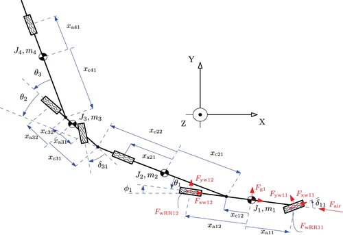
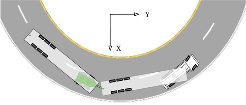
The vehicle considered in this paper is an A-double, i.e. a four-unit LCV that is a tractor-semitrailer-dolly-semitrailer. It is modelled as a nonlinear single-track vehicle, as shown in Figure 1, including a nonlinear tyre model and considering the combined slip. The single-track models capture the important vehicle dynamics behaviours that are sufficient for trajectory tracking and motion planning in normal driving conditions, e.g. the lateral acceleration up to 2 $\frac{\mathrm{m}}{{\mathrm{s}}^2}$. Ghandriz et al. [58] validated the nonlinear single-track model using the experimental data with different driving manoeuvrers.

Figure 1. Single-track representation of an A-double. The figure illustrates the vehicle dimensions, i.e. the axle positions $x_{\mathrm{a}ij}$, units front coupling positions $x_{\mathrm{c}i1}$, and units rear coupling positions $x_{\mathrm{c}i2}$ relative to the units COGs, where, i and j are unit and axle indices, respectively. Moreover, the figure shows the articulation angles ${\theta }_i$ between unit i and i + 1, steering angles ${\delta }_{ij}$, units masses $m_i$, units moments of inertia $J_i$ and the examples of the forces acting on the vehicle, i.e. the axles longitudinal forces from the propulsion/braking actuation $F_{\mathrm{xw}ij}$, the lateral forces $F_{\mathrm{yw}ij}$, air resistance $F_{\mathrm{air}}$, rolling resistance forces $F_{\mathrm{wRR}ij}$ and the gravitational forces caused by road banking $F_{\mathrm{g}i}$.

The derivation of the vehicle nonlinear dynamic equation by using Lagrangian mechanics is presented in Appendix 1 and is based on [58]. The benefit of using the Lagrangian mechanics is that the dynamic equation can be derived in the minimum order, i.e. with the least number of states and equations. We used the following assumptions during the derivation of the vehicle model:

–	the motion is limited to the yaw-plane, i.e. the roll-motion has a negligible effect;
–	the articulation joints are yaw moment-free with no friction;
–	the propulsion and brake actuation inputs are axle forces on the ground plane rather than the engine or electric motors torques, and they are same on the right and left sides such that they do not create a yaw moment;
–	a longitudinal wheel slip controller provides the requested longitudinal force by controlling the longitudinal slip so that the wheel rotational inertia is handled by this controller;
–	the air resistance force acts only on the front ground level of the first unit, and no other aerodynamic force is modelled;
–	there is no actuator delay;
–	the vehicle longitudinal speed cannot be zero.

The nonlinear dynamic equation of the vehicle is a system of implicit ordinary differential equations (ODEs) or a differential algebraic equations (DAEs) in the form of (1) $F(x(s),\frac{\mathrm{d}x(s)}{\mathrm{d}s},u(s),s)=0,$(1) where s is the distance travelled, and x and u are the state and input vectors, respectively. The independent variable of the dynamic system (1(1) $F(x(s),\frac{\mathrm{d}x(s)}{\mathrm{d}s},u(s),s)=0,$(1) ) is the distance travelled s rather than the time t, because the road curvature and grade are described by s.

In (1(1) $F(x(s),\frac{\mathrm{d}x(s)}{\mathrm{d}s},u(s),s)=0,$(1) ), the state vector is (2) $x=[X_1,Y_1,{\varphi }_1,{\theta }_1,{\theta }_2,{\theta }_3,v_{\mathrm{x}1},v_{\mathrm{y}1},\frac{\mathrm{d}{\varphi }_1}{\mathrm{d}s},\frac{\mathrm{d}{\theta }_1}{\mathrm{d}s},\frac{\mathrm{d}{\theta }_2}{\mathrm{d}s},\frac{\mathrm{d}{\theta }_3}{\mathrm{d}s}],$(2) where $X_1$ and $Y_1$ are the global coordinates of the first units' COG, ${\varphi }_1$ is the angle of the first unit with respect to the global Y -axis, $v_{\mathrm{x}1}$ and $v_{\mathrm{y}1}$ are the velocity components of the first unit's COG in the first unit's local system of coordinates, and ${\theta }_1$, ${\theta }_2$, and ${\theta }_3$ are the articulation angles as shown in Figure 1. We defined the input vector as (3) $u=[F_{\mathrm{xw}11},F_{\mathrm{xw}12},F_{\mathrm{xw}21},F_{\mathrm{xw}31},F_{\mathrm{xw}32},F_{\mathrm{xw}41},{\delta }_{11},{\delta }_{31}],$(3) where $F_{\mathrm{xw}jr}$ is the $j^{\mathrm{th}}$ unit's $r^{\mathrm{th}}$ grouped-axle longitudinal force caused by the propulsion or braking actuation, ${\delta }_{11}$ is the steering angle of the first axle of the first unit, and ${\delta }_{31}$ is the steering angle of the first axle of the third unit, i.e. the steering angle of the dolly converter. The axle propulsion is provided either by engine or by electric motors.

It should be noted that the system dynamic equation is implicit since the explicit form derived for the four-unit subject vehicle in this paper has substantially more terms than the implicit form, making the Jacobian evaluation computationally expensive.

4. NMPC problem formulation

The nonlinear optimal control problem in the continuous form is defined as (4a) $\begin{array}{rlrl}& \text{find}& & u(s),s\in [s_0,s_e[\\ & \text{to minimise}& & \overline{C}=C_{\mathrm{t}}(x(s_e),s_e)+{\int }_{s_0}^{s_e}L(x(s),u(s),s)\mathrm{d}s,\\ & \text{subject to}& & F(x(s),\frac{\mathrm{d}x(s)}{\mathrm{d}s},u(s),s)=0,\end{array}$(4a) (4c) $\begin{array}{rlrl}& & & h(x(s),\frac{\mathrm{d}x(s)}{\mathrm{d}s},u(s),s)\le 0,\end{array}$(4c) $\begin{array}{rlrl}& & & x(0)=x_{\mathrm{init}},\end{array}$ where $\overline{C}$ is the cost function, $C_{\mathrm{t}}$ is the terminal cost, L is the stage cost, F is the vehicle dynamic equation constraint, h is a function representing the limits on states and inputs, as well as, e.g. actuators and path limits, $x_{\mathrm{init}}$ is the initial state, and $s_0$ and $s_e$ are the start and end distances, respectively.

We first perform the discretisation and then the linearisation of the optimal control problem (4) for constructing an NMPC. Then, we solve the NMPC by using the SQP or LTV-MPC approaches [24]. We discretise the space to a equidistant grid with a step size $\mathrm{\Delta }s$ assuming a zero-order-holder that maintains the controls constant within a discretisation step. The system derivatives must be approximated using a numerical method. While the explicit Euler method is the most straightforward approximation, it is inefficient and for a large step size $\mathrm{\Delta }s$ it may become unstable. Multistep methods can also be used, but they require additional care for initialisation. On the other hand, Runge–Kutta methods are not suitable for implicit ODEs such as (1(1) $F(x(s),\frac{\mathrm{d}x(s)}{\mathrm{d}s},u(s),s)=0,$(1) ). Therefore, we used the Euler approximation in this paper, i.e. (5) ${\frac{\mathrm{d}x}{\mathrm{d}s}}^k=\frac{x^{k+1}-x^k}{\mathrm{\Delta }s},$(5) where, in this paper, for $\mathrm{\Delta }s\le 1$ m, the numerical solution is stable, and the system Jacobian defined in later sections is not singular. Larger step size than 1 m might result in singular Jacobian and hence divergence of the numerical solution depending on the selected manoeuvrer.

We assume that the stage cost L is (or can be approximated as) a quadratic convex function of the states and inputs. Then, we define the discretised form of the NMPC at distance step i, and for the prediction horizon of length N, as (6a) $\begin{array}{rlrl}& \text{find}& & x^{i(k+1)},u^{ik},k=0,\dots ,N-1\\ & \text{to minimise}& & {\overline{C}}^i=C_{\mathrm{t}}(x^{iN},x_{\mathrm{des}}^{iN})+\\ & & & \sum _{k=0}^{N-1}{\left[\begin{array}{c}{x}^{ik}-x_{\mathrm{des}}^{ik}\\ u^{ik}-u_{\mathrm{des}}^{ik}\end{array}\right]}^T{W}_{ik}\left[\begin{array}{c}{x}^{ik}-x_{\mathrm{des}}^{ik}\\ u^{ik}-u_{\mathrm{des}}^{ik}\end{array}\right]\end{array}$(6a) (6b) $\begin{array}{rlrl}& \text{subject to}& & \mathrm{for}k=0,\dots ,N-1,\\ & & & F(x^{ik},\frac{x^{i(k+1)}-x^{ik}}{\mathrm{\Delta }s},u^{ik},k)=0,\end{array}$(6b) (6c) $\begin{array}{rlrl}& & & h(x^{ik},\frac{x^{i(k+1)}-x^{ik}}{\mathrm{\Delta }s},u^{ik},k)\le 0,\\ & & & x^{i0}={\hat{x}}^i,\end{array}$(6c) where the first term of ${\overline{C}}^i$ is the terminal cost, subscript ‘${}_{\mathrm{des}}$’ indicates the desired path, $W_{ik}$ is a weighting positive semidefinite matrix, and ${\hat{x}}^i$ is the state estimate at distance step i. We note that in (6), we used the same notation as in the continuous optimal control problem (4).

4.1. NMPC solution using SQP

The system dynamic equation can be linearised using different methods. A common approach in the literature that results in an STL model is to simplify the system by assuming small angles and removing all high-order terms. STL models are limited to exclusively steering control and constant longitudinal speed and small angles. Another approach for linearisation is to simplify the equations by assuming small angles and then to carry out linearisation around the operating point at the current state. Therefore, the optimal control problem can be implemented for a very short horizon, usually for less than 1 s or 15 m. For longer prediction horizons, the linearised prediction model becomes inaccurate.

An alternative approach is to linearise the nonlinear system dynamics around an IGRTL without performing any simplifications. The IGRTL can be either the same as the desired trajectory, can be obtained by a simpler computationally efficient controller, or can be taken from a set of the previously saved references in an look-up table for specific manoeuvrers and driving conditions, e.g. payloads. This approach makes the combined steering, braking and propulsion optimal control possible in long horizons with varying road curvature and vehicle states.

The linear dynamic equation can be derived by using the first-order Taylor expansion of (6b(6b) $\begin{array}{rlrl}& \text{subject to}& & \mathrm{for}k=0,\dots ,N-1,\\ & & & F(x^{ik},\frac{x^{i(k+1)}-x^{ik}}{\mathrm{\Delta }s},u^{ik},k)=0,\end{array}$(6b) ) around the guess states and inputs $[x_0^{ik},u_0^{ik},x_0^{iN}]$, $k=0,\dots ,N-1$, as described by (7) $\begin{array}{rl}& F_{\mathrm{lin}}(x^{i(k+1)},x^{ik},u^{ik},k)=\\ & F(x_0^{i(k+1)},x_0^{ik},u_0^{ik},k)\\ & +J_F(x^{i(k+1)}){|}_{(x_0^{i(k+1)},x_0^{ik},u_0^{ik})}(x^{i(k+1)}-x_0^{i(k+1)})\\ & +J_F(x^{ik}){|}_{(x_0^{i(k+1)},x_0^{ik},u_0^{ik})}(x^{ik}-x_0^{ik})\\ & +J_F(u^{ik}){|}_{(x_0^{i(k+1)},x_0^{ik},u_0^{ik})}(u^{ik}-u_0^{ik})=0,\\ & k=0,\dots ,N-1,\end{array}$(7) where $J_F(\cdot )$ is the Jacobian matrix of F, whose entries are defined as, e.g. for a vector argument y, $J_{Fjl}(y)=\frac{\mathrm{\partial }{F}_j}{\mathrm{\partial }{y}_l},j=1,\dots ,N,l=1,\dots ,M$, where N is the number of single functions in F, and M is the number of function arguments, i.e. the size of the y vector.

Note that if the guess states and inputs satisfy the system dynamics, then the term $F(x_0^{i(k+1)},x_0^{ik},u_0^{ik})$ is equal to zero.

Let us define (8) $\begin{array}{rl}& y^{ik}=[x^{i(k+1)},x^{ik},u^{ik}{]}^T\\ & y_0^{ik}=[x_0^{i(k+1)},x_0^{ik},u_0^{ik}{]}^T.\end{array}$(8) Then, (7(7) $\begin{array}{rl}& F_{\mathrm{lin}}(x^{i(k+1)},x^{ik},u^{ik},k)=\\ & F(x_0^{i(k+1)},x_0^{ik},u_0^{ik},k)\\ & +J_F(x^{i(k+1)}){|}_{(x_0^{i(k+1)},x_0^{ik},u_0^{ik})}(x^{i(k+1)}-x_0^{i(k+1)})\\ & +J_F(x^{ik}){|}_{(x_0^{i(k+1)},x_0^{ik},u_0^{ik})}(x^{ik}-x_0^{ik})\\ & +J_F(u^{ik}){|}_{(x_0^{i(k+1)},x_0^{ik},u_0^{ik})}(u^{ik}-u_0^{ik})=0,\\ & k=0,\dots ,N-1,\end{array}$(7) ) can be written as (9) $F(y_0^{ik})+J_F(y^{ik}){|}_{y_0^{ik}}(y^{ik}-y_0^{ik})=0.$(9) If the cost function is not convex and quadratic, then it should be approximated by a quadratic convex function around the guess states and inputs $[x_0^{ik},u_0^{ik},x_0^{iN}]$, $k=0,\dots ,N-1$, [59]. However, in this paper, we assumed a convex and quadratic cost function given the desired trajectory.

Let us define $\begin{array}{rlr}& {\mathit{x}}^i=[x^{i0},x^{i1},x^{i2},\dots ,x^{iN}]& {\mathit{u}}^i=[u^{i0},u^{i1},u^{i2},\dots ,u^{i(N-1)}].\end{array}$ After performing the same linearisation steps (7(7) $\begin{array}{rl}& F_{\mathrm{lin}}(x^{i(k+1)},x^{ik},u^{ik},k)=\\ & F(x_0^{i(k+1)},x_0^{ik},u_0^{ik},k)\\ & +J_F(x^{i(k+1)}){|}_{(x_0^{i(k+1)},x_0^{ik},u_0^{ik})}(x^{i(k+1)}-x_0^{i(k+1)})\\ & +J_F(x^{ik}){|}_{(x_0^{i(k+1)},x_0^{ik},u_0^{ik})}(x^{ik}-x_0^{ik})\\ & +J_F(u^{ik}){|}_{(x_0^{i(k+1)},x_0^{ik},u_0^{ik})}(u^{ik}-u_0^{ik})=0,\\ & k=0,\dots ,N-1,\end{array}$(7) )–(9(9) $F(y_0^{ik})+J_F(y^{ik}){|}_{y_0^{ik}}(y^{ik}-y_0^{ik})=0.$(9) ) for h in (6c(6c) $\begin{array}{rlrl}& & & h(x^{ik},\frac{x^{i(k+1)}-x^{ik}}{\mathrm{\Delta }s},u^{ik},k)\le 0,\\ & & & x^{i0}={\hat{x}}^i,\end{array}$(6c) ), the quadratic programme (QP, or the LTV-MPC) can be written as ${\mathrm{QP}}_{\mathrm{NMPC}}({\hat{x}}^i,{\mathit{x}}_0^i,{\mathit{u}}_0^i,{\mathit{x}}_{\mathrm{des}}^i,{\mathit{u}}_{\mathrm{des}}^i)=$ (10a) $\begin{array}{rlrl}& \text{find}& & x^{i(k+1)},u^{ik},k=0,\dots ,N-1\\ & \text{to minimise}& & {\overline{C}}^i=C_{\mathrm{t}}(x^{iN},x_{\mathrm{des}}^i)+\\ & & & \sum _{k=0}^{N-1}{\left[\begin{array}{c}{x}^{ik}-x_{\mathrm{des}}^{ik}\\ u^{ik}-u_{\mathrm{des}}^{ik}\end{array}\right]}^T{W}_{ik}\left[\begin{array}{c}{x}^{ik}-x_{\mathrm{des}}^{ik}\\ u^{ik}-u_{\mathrm{des}}^{ik}\end{array}\right]\end{array}$(10a) (10b) $\begin{array}{rlrl}& \text{subject to}& & \mathrm{for}k=0,\dots ,N-1\\ & & & F(y_0^{ik})+J_F(y^{ik}){|}_{y_0^{ik}}(y^{ik}-y_0^{ik})=0,\end{array}$(10b) (10c) $\begin{array}{rlrl}& & & h(y_0^{ik})+J_h(y^{ik}){|}_{y_0^{ik}}(y^{ik}-y_0^{ik})\le 0,\\ & & & y^{ik}=[x^{i(k+1)},x^{ik},u^{ik}{]}^T\\ & & & y_0^{ik}=[x_0^{i(k+1)},x_0^{ik},u_0^{ik}{]}^T\\ & & & x^{i0}={\hat{x}}^i.\end{array}$(10c)

The optimal control problem defined in (10) is an LTV-MPC. The solution of the LTV-MPC problem ${\mathrm{QP}}_{\mathrm{NMPC}}({\hat{x}}^i,{\mathit{x}}_0^i,{\mathit{u}}_0^i,{\mathit{x}}_{\mathrm{des}}^i,{\mathit{u}}_{\mathrm{des}}^i)$ can be used to define a new states-inputs guess $[{\mathit{x}}_1^i,{\mathit{u}}_1^i]$. The NMPC can then be linearised again around the new guess to define a new LTV-MPC ${\mathrm{QP}}_{\mathrm{NMPC}}({\hat{x}}^i,{\mathit{x}}_1^i,{\mathit{u}}_1^i,{\mathit{x}}_{\mathrm{des}}^i,{\mathit{u}}_{\mathrm{des}}^i)$. Continuing this procedure forms the SQP that gives the solution of the NMPC upon convergence [24], according to Algorithm 1.

The SQP is computationally expensive for most of the real-time NMPC applications. The number of sequential iterations; i.e. the iterations in Algorithm 1 prior to convergence indicates the quality of the chosen initial linearisation guess trajectory. It can be reduced if the SQP is warm-started. The RTI method is an efficient approach for solving an NMPC where Algorithm 1 is iterated only once at distance-step i by using a full Newton step, $\alpha =1$. The solution is then used as a warm, i.e. good-quality, linearisation guess for the NMPC linearisation at distance-step $(i+1)$ [23,24]. RTI reduces the computational cost of SQP considerably; however, step 2 of Algorithm 1, i.e. evaluating the Jacobians and linearisation of constraints, must be performed online. This step is computationally expensive for the nonlinear vehicle model of the articulated vehicles, e.g. the A-double model used in this paper. To overcome this problem, we proposed to perform step 2 of Algorithm 1 off-line by using an off-line linearisation guess that is relatively close to the NMPC solution.

4.2. LTV-MPC and off-line linearisation

Algorithm 1 solves an LTV-MPC, if it is executed with a single iteration, and for a full Newton step, $\alpha =1$. Algorithm 2 describes the LTV-MPC, where the NMPC linearisation is performed off-line.

Algorithm 2 provides a solution close the solution of Algorithm 1 if either the initial linearisation guess is good or the system dynamics equation is not highly nonlinear. In the following, we study the level of the nonlinearity of the dynamic equation of motion of the chosen articulated vehicle by examining the number of iterations prior to convergence in the open-loop simulations and closed-loop control.

5. Open-loop simulations

In this paper, open-loop simulation refers to the integration of the system of ODEs where the inputs u are known in advance and no optimisation of the trajectories is performed. In this section, we provide examples of the IGRTL of the LCV motion that yield the solution of system of ODEs by a single iteration of the Newton method.

Sequential programming is based on Newton's iterations used for finding a root of a function, e.g. $F(x)$. (11) $x_{j+1}=x_j-\frac{F(x_j)}{J_F(x){|}_{x_j}},$(11) where x is the function argument. If $||x_{j+1}-x_j||\le ϵ$, the convergence is reached and $x_j$ can be taken as a root of the function system F, where ϵ is a small number. In (11(11) $x_{j+1}=x_j-\frac{F(x_j)}{J_F(x){|}_{x_j}},$(11) ), $x_0$ is the initial guess. We note that (11(11) $x_{j+1}=x_j-\frac{F(x_j)}{J_F(x){|}_{x_j}},$(11) ) has the same form as (9(9) $F(y_0^{ik})+J_F(y^{ik}){|}_{y_0^{ik}}(y^{ik}-y_0^{ik})=0.$(9) ) where we redefined the function argument.

DAE solvers commonly use Newton-type methods for solving DAEs [63]. In this case, the unknowns are algebraic variables, states, and the state derivatives that must be expressed in terms of the states. If no analytical solution is available, which is the case for most problems, the problem must be discretised, and the state derivatives must be approximated by a difference formula such as Euler, Runge–Kutta, or backward differentiation. Therefore, the DAE solution also depends on the discretisation method used and its properties. The Newton's method combined with the integration (in distance) of the implicit ODE equations (6b(6b) $\begin{array}{rlrl}& \text{subject to}& & \mathrm{for}k=0,\dots ,N-1,\\ & & & F(x^{ik},\frac{x^{i(k+1)}-x^{ik}}{\mathrm{\Delta }s},u^{ik},k)=0,\end{array}$(6b) ) can be expressed according to the following at distance-step k, where the inputs $u^k$ are known in an open-loop simulation: (12) $x_{j+1}^k=x_j^k-\frac{F(x_j^k)}{{\mathit{J}}_F(x^k){|}_{x_j^k}},$(12) where $x_0^0$ is the initial condition of the integration, which is the same as the Newton's method initial guess at the first distance-step, and j denotes the iteration number. At distance-step k + 1, the converged solution of the previous distance-step works as an initial guess for the Newton's iteration, i.e. $x_0^{k+1}=x^k$.

The objective of the above introduction lies in the following. Instead of integrating (12(12) $x_{j+1}^k=x_j^k-\frac{F(x_j^k)}{{\mathit{J}}_F(x^k){|}_{x_j^k}},$(12) ) forward in distance, all the initial guesses of all the distance-steps $x_0^k$, for $k=0,\dots ,N$ can be gathered in a global vector ${\mathit{x}}_0$, and the same procedure can be performed for the known inputs to form the global input vector $\mathit{u}$. Consequently, the global system of equations $\mathit{F}$ of all the distance-steps with the corresponding Jacobian matrix ${\mathit{J}}_{\mathit{F}}$ can be defined such that (13) ${\mathit{x}}_{j+1}={\mathit{x}}_j-\frac{\mathit{F}({\mathit{x}}_j)}{{\mathit{J}}_{\mathit{F}}(\mathit{x}){|}_{{\mathit{x}}_j}},$(13) where ${\mathit{x}}_0$ is the IGRTL. If convergence is reached, i.e. if $||{\mathit{x}}_{j+1}-{\mathit{x}}_j|{|}^2\le ϵ$, then the global vector ${\mathit{x}}_j$ contains the solution of the implicit ODE (or the DAE), i.e. the same solution that can be obtained by solving (12(12) $x_{j+1}^k=x_j^k-\frac{F(x_j^k)}{{\mathit{J}}_F(x^k){|}_{x_j^k}},$(12) ).

The main benefit of solving the problem in the form given by (13(13) ${\mathit{x}}_{j+1}={\mathit{x}}_j-\frac{\mathit{F}({\mathit{x}}_j)}{{\mathit{J}}_{\mathit{F}}(\mathit{x}){|}_{{\mathit{x}}_j}},$(13) ) is that $\mathit{F}({\mathit{x}}_0)$ and ${\mathit{J}}_{\mathit{F}}(\mathit{x}){|}_{{\mathit{x}}_0}$ can be calculated off-line in advance so that if a good initial guess ${\mathit{x}}_0$ is selected, the final solution can be found by a single iteration, that is, by solving (13(13) ${\mathit{x}}_{j+1}={\mathit{x}}_j-\frac{\mathit{F}({\mathit{x}}_j)}{{\mathit{J}}_{\mathit{F}}(\mathit{x}){|}_{{\mathit{x}}_j}},$(13) ) only once. Moreover, if more iterations are needed, the solution can still be obtained more efficiently than that obtained by the distance-integration according to (12(12) $x_{j+1}^k=x_j^k-\frac{F(x_j^k)}{{\mathit{J}}_F(x^k){|}_{x_j^k}},$(12) ).

It should be noted that the singularity of the global Jacobian matrix can be avoided by removing the rows and columns corresponding to the known states and moving them to the right-hand side, i.e. by adding them to $\mathit{F}$.

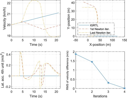
The importance of a good choice of the IGRTL is studied using two different driving manoeuvrers for the nonlinear single-track four-unit and six-axle A-double LCV model. The manoeuvrers are a single-lane change and a U-turn. If the IGRTL are far from the nonlinear solution, a single Newton iteration does not provide a solution close to the nonlinear solution.

5.1. Examples of ‘bad’ initial guesses

A simple linearisation is a linearisation around zero steering inputs and a constant (or zero) braking and propulsion forces. Examples are shown in Figures 2 and 3. In these figures, the IGRTL comprises the vehicle states when the vehicle drives straight, i.e. with no steering input. This means that no information about the manoeuvrer was used to generate the IGRTL. The convergence is reached if the root mean square (RMS) of the velocity difference between the two successive iterations is less than 0.1 $\frac{\mathrm{m}}{\mathrm{s}}$. We selected these convergence criteria because the error of a lower level driver model for controlling the speed is more than 0.1 $\frac{\mathrm{m}}{\mathrm{s}}$ [64]. It is observed from Figures 2 and 3 that two and four Newton iterations are necessary to obtain the nonlinear solution of the vehicle equation of motion for the single-lane change and U-turn manoeuvrers, respectively, starting from the given linearisation guesses.

Figure 2. A single-lane-change manoeuvrer. Comparison of the different vehicle states (at COG) obtained by the two different solution methods: the nonlinear method (given by the last Newton iteration) and linear method (given by the first Newton iteration). The lower right plot shows the convergence of the linear solution to the nonlinear solution by performing Newton iterations in terms of the RMS of the velocity difference ($\frac{\mathrm{m}}{\mathrm{s}}$) between the two successive Newton iterations. The IGRTL comprises the states of a vehicle that drives straight with zero steering, braking and propulsion inputs.

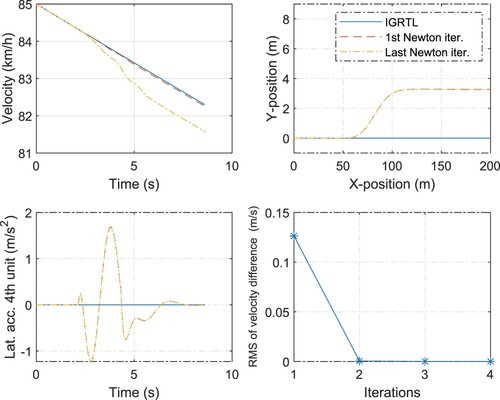
Figure 3. A U-turn manoeuvrer. Comparison of the different vehicle states (at COG) obtained by the two different solution methods: the nonlinear method (given by the last Newton iteration) and linear method (given by the first Newton iteration). The lower right plot shows the convergence of the linear solution to the nonlinear solution in terms of the RMS of the velocity difference ($\frac{\mathrm{m}}{\mathrm{s}}$) between the two successive Newton iterations. The IGRTL comprises the states of a vehicle that drives straight. The propulsion input $F_{\mathrm{xw}12=20}$ kN is the same for all the cases.

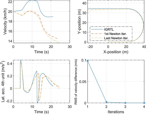
5.2. Examples of ‘good’ initial guesses

If the selected IGRTL is close to the nonlinear solution then the solution of the linearised problem, i.e. the solution obtained after the first Newton iteration, is relatively close to the nonlinear solution, satisfying the convergence criteria, as seen in Figures 4 and 5. The IGRTL comprises the states of a vehicle driving in a sample manoeuvrer rather than in the straight road driving. Moreover, the IGRTL does not need to be ‘so close’ to the nonlinear solution in order to reach the convergence by a single Newton iteration. As observed from the figures, the velocity of the IGRTL is different from the nonlinear solution. In addition, the IGRTL can be generated with the different inputs than those used in the modelled vehicle. If the difference in the inputs is not ‘large’ then the linearised model can result in a solution very close to that of the nonlinear model, as shown in Figures 6 and 7, where the modelled vehicle brakes during the manoeuvrer.

Figure 4. A single-lane-change manoeuvrer. Comparison of the different vehicle states (at COG) obtained by the two different solution methods: the nonlinear method (given by the last Newton iteration) and linear method (given by the first Newton iteration). The IGRTL comprises the states of a vehicle that drives in a sample (or guessed) single-lane-change manoeuvrer with no braking and propulsion. The reference vehicle used for generating IGRTL and the vehicle simulated by performing Newton iterations have the same steering inputs but different velocities.

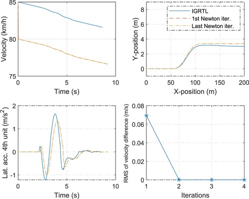
Figure 5. A U-turn manoeuvrer. Comparison of the different vehicle states (at COG) obtained by the two different solution methods: the nonlinear method (given by the last Newton iteration) and linear method (given by the first Newton iteration). The IGRTL comprises the states of a vehicle that drives in a sample (or guessed) U-turn manoeuvrer. The steering and propulsion inputs are the same in the reference vehicle used for generating IGRTL and in the vehicle simulated by performing Newton iterations, but they have different velocities.

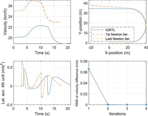
Figure 6. A single-lane-change manoeuvrer. Comparison of the different vehicle states (at COG) obtained by the two different solution methods: the nonlinear method (given by the last Newton iteration) and linear method (given by the first Newton iteration). The IGRTL comprises the states of a vehicle that drives in a sample (or guessed) single-lane-change manoeuvrer with no braking and propulsion. The reference vehicle used for generating IGRTL and the vehicle simulated by performing Newton iterations have the same steering inputs. However, the vehicle was simulated by performing Newton iterations brakes in some axles.

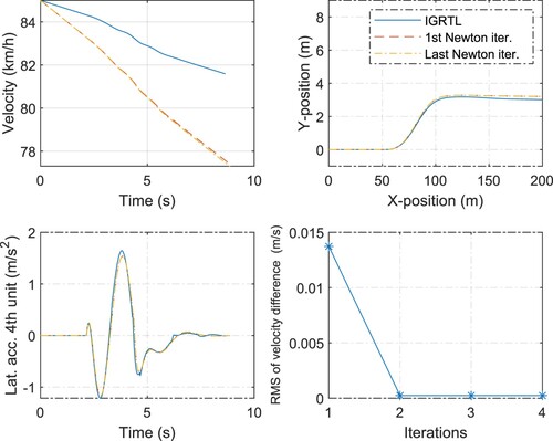
Figure 7. A U-turn manoeuvrer. Comparison of the different vehicle states (at COG) obtained by the two different solution methods: the nonlinear method (given by the last Newton iteration) and linear method (given by the first Newton iteration). The IGRTL comprises the states of a vehicle that drives in a sample (or guessed) U-turn manoeuvrer. The steering and propulsion inputs of the reference vehicle used for generating IGRTL and the vehicle simulated by performing Newton iterations are the same, but they have different velocities. However, the vehicle simulated by performing Newton iterations brakes in some axles.

Therefore, according to the above discussion, MPC controllers can be designed by using the linearised system of equations of motion of the articulated vehicles with no need of sequential iterations of the linearised system, if a ‘good’ IGRTL is selected. How ‘good’ depends on the manoeuvrer, driving cycle and the controlled inputs. For instance, if a representative driving cycle is known, the reference state trajectories that is used for linearising the nonlinear system of equations, i.e. IGRTL, can be generated by solving the nonlinear equations only once off-line, for the given driving cycle, and by using a simple control law. Then, an advanced MPC controller can be designed for improving the control law by using the linearised system of equations. Some deviation from the linearisation reference states-inputs, caused by, e.g. disturbances, does not invalidate the linearised equations.

6. Trajectory-following and off-tracking minimisation of LCVs by using NMPC and LTV-MPC

6.1. NMPC formulation

Off-tracking is a maximum deviation of the path of the vehicle units (or axles) compared to the path of the first unit (or the first axle). It is one of the measures for the evaluation and standardisation of LCVs performance on the road [20,65,66]. Minimisation of the off-tracking is an application of the optimal control problem defined in (10). We define the stage cost function in the space domain as (14) $\begin{array}{rl}& L(x(s),u(s),s)=\sum _{i=1}^{n_{\mathrm{u}}}((X_i(x(s),s)-X_{\mathrm{des}i}(s){)}^T{H}_{\mathrm{X}}(X_i(x(s),s)-X_{\mathrm{des}i}(s))\\ & +(Y_i(x(s),s)-Y_{\mathrm{des}i}(s){)}^T{H}_{\mathrm{Y}}(Y_i(x(s),s)-Y_{\mathrm{des}i}(s))),\end{array}$(14) with a generalisation that the stage cost also includes the deviation cost of the first unit from its own path, where $n_{\mathrm{u}}$ is the number of vehicle units, $[X_i,Y_i]$ are the global coordinates of unit i COG, $[X_{\mathrm{des}i},Y_{\mathrm{des}i}]$ are the global coordinates of the desired path of COGs, and $H_{\mathrm{X}}$ and $H_{\mathrm{Y}}$ are the weighting matrices. The objective is to reduce the distance between the trajectory of all the units and the given desired trajectory. We assumed that the desired trajectory of the first unit is known either from the road, or by simulating the nonlinear vehicle motion using a simple driver model for controlling the steering of the first axle, and for a specific manoeuvrer. Therefore, given the desired trajectory of the COG of the first unit $[X_{\mathrm{des}1},Y_{\mathrm{des}1}]$, the desired trajectories of COGs of the other units can be defined as (15) $\begin{array}{rl}& X_{\mathrm{des}i}(s)=X_{\mathrm{des}1}(s_i),i=2,\dots ,n_{\mathrm{u}}\\ & Y_{\mathrm{des}i}(s)=Y_{\mathrm{des}1}(s_i),i=2,\dots ,n_{\mathrm{u}},\end{array}$(15) where (16) $s_i=s+\sum _{l=1}^{i-1}{x}_{\mathrm{c}l2}-\sum _{l=2}^i{x}_{\mathrm{c}l1},i=2,\dots ,n_{\mathrm{u}},$(16) where $x_{\mathrm{c}l1}$ and $x_{\mathrm{c}l2}$ are the vehicle unit local x-coordinates of the front and rear coupling points relative to the unit's COG, respectively.

Moreover, $[X_i,Y_i]$ are nonlinear functions of states. These must be linearised around the IGRTL in order to make the cost function convex and quadratic and suitable for defining the ${\mathrm{QP}}_{\mathrm{NMPC}}$ problem. The IGRTL can be defined using a simple vehicle controller following the desired trajectory.

Let us discretise the space and define (17) ${\overline{y}}^k(x^k,k)=[X_1(x^k,k),Y_1(x^k,k),\dots ,X_{n_u}(x^k,k),Y_{n_u}(x^k,k){]}^T,k=0,\dots ,N,$(17) and (18) ${\overline{y}}_{\mathrm{des}}^k=[X_{\mathrm{des}1}^k,Y_{\mathrm{des}1}^k,\dots ,X_{\mathrm{des}{n}_{\mathrm{u}}}^k,Y_{\mathrm{des}{n}_{\mathrm{u}}}^k{]}^T,k=0,\dots ,N.$(18) The linearisation of ${\overline{y}}^k$ by finding its Jacobian with respect to state $x^k$ evaluated at $x_0^k$ yields (19) ${\overline{y}}_{\mathrm{lin}}^k(x^k,k)={\overline{A}}_0^k{x}^k+{\overline{b}}_0^k.$(19) Then, the state cost function (14(14) $\begin{array}{rl}& L(x(s),u(s),s)=\sum _{i=1}^{n_{\mathrm{u}}}((X_i(x(s),s)-X_{\mathrm{des}i}(s){)}^T{H}_{\mathrm{X}}(X_i(x(s),s)-X_{\mathrm{des}i}(s))\\ & +(Y_i(x(s),s)-Y_{\mathrm{des}i}(s){)}^T{H}_{\mathrm{Y}}(Y_i(x(s),s)-Y_{\mathrm{des}i}(s))),\end{array}$(14) ) can be written as (20) $L(x^k,u^k)=({\overline{A}}_0^k{x}^k+{\overline{b}}_0^k-{\overline{y}}_{\mathrm{des}}^k{)}^{T}H({\overline{A}}_0^k{x}^k+{\overline{b}}_0^k-{\overline{y}}_{\mathrm{des}}^k),$(20) where H is a positive semidefinite weighting matrix. Rearranging the terms and removing the constants yield (21) $L(x^k,u^k)=(x^k{)}^T({\overline{A}}_0^k{)}^{T}H{\overline{A}}_0^k{x}^k-2({\overline{y}}_{\mathrm{des}}^k-{\overline{b}}_0^k{)}^{T}H{\overline{A}}_0^k{x}^k.$(21) Therefore, the off-tracking minimisation ${\mathrm{QP}}_{\mathrm{NMPC}}$ problem for a single-track A-double with a steerable dolly, where the whole manoeuvrer is considered a single prediction horizon of N discrete stages can be written as follows. (22a) $\begin{array}{rlrl}& \text{find}& & x^{(k+1)},u^k,k=0,\dots ,N-1\\ & \text{to minimise}& & \sum _{k=0}^N((x^k{)}^T({\overline{A}}_0^k{)}^{T}H{\overline{A}}_0^k{x}^k-\\ & & & 2({\overline{y}}_{\mathrm{des}}^k-{\overline{b}}_0^k{)}^{T}H{\overline{A}}_0^k{x}^k),\end{array}$(22a) (22b) $\begin{array}{rlrl}& \text{subject to}& & \mathrm{for}k=0,\dots ,N-1\\ & & & F(y_0^k)+J_F(y^k){|}_{y_0^k}(y^k-y_0^k)=0,\end{array}$(22b) (22c) $\begin{array}{rlrl}& & & y^k=[x^{(k+1)},x^k,u^k{]}^T,\\ & & & y_0^k=[x_0^{(k+1)},x_0^k,u_0^k{]}^T,\\ & & & x_{min}^{k+1}\le x^{k+1}\le x_{max}^{k+1},\end{array}$(22c) (22d) $\begin{array}{rlrl}& & & u_{min}^k\le u^k\le u_{max}^k,\\ & & & x^0={\hat{x}}^0,\end{array}$(22d) where constraint (22b(22b) $\begin{array}{rlrl}& \text{subject to}& & \mathrm{for}k=0,\dots ,N-1\\ & & & F(y_0^k)+J_F(y^k){|}_{y_0^k}(y^k-y_0^k)=0,\end{array}$(22b) ) is for the linearised system dynamics and the same as in (10b(10b) $\begin{array}{rlrl}& \text{subject to}& & \mathrm{for}k=0,\dots ,N-1\\ & & & F(y_0^{ik})+J_F(y^{ik}){|}_{y_0^{ik}}(y^{ik}-y_0^{ik})=0,\end{array}$(10b) ), and constraints (22c(22c) $\begin{array}{rlrl}& & & y^k=[x^{(k+1)},x^k,u^k{]}^T,\\ & & & y_0^k=[x_0^{(k+1)},x_0^k,u_0^k{]}^T,\\ & & & x_{min}^{k+1}\le x^{k+1}\le x_{max}^{k+1},\end{array}$(22c) ) and (22d(22d) $\begin{array}{rlrl}& & & u_{min}^k\le u^k\le u_{max}^k,\\ & & & x^0={\hat{x}}^0,\end{array}$(22d) ) bound the states and inputs.

Furthermore, the states can be solved for the inputs by using constraint (22b(22b) $\begin{array}{rlrl}& \text{subject to}& & \mathrm{for}k=0,\dots ,N-1\\ & & & F(y_0^k)+J_F(y^k){|}_{y_0^k}(y^k-y_0^k)=0,\end{array}$(22b) ). Moreover, cost function and constraints could include terms to penalise or limit the rate of the inputs, as well as the proximity to the road sides and road users, which would change the problem to a motion planning problem rather than the trajectory-tracking. Moreover, to avoid close-to-roll-over situations in high-speed manoeuvrers, where following the desired trajectory would cause a high lateral acceleration, constraints on lateral acceleration can be added for each of the vehicle units [67].

It should be noted that the controller is NMPC which, through nonlinear vehicle model, automatically adjusts to different dynamics and speeds. Moreover, for LTV-MPC, we use different linearised systems for different dynamics and speeds. Therefore, a similar gain matrix (identity matrix in our case) could be used both in low- and high-speed manoeuvrers.

6.2. Results of NMPC and LTV-MPC

The trajectory-following and off-tracking minimisation ${\mathrm{QP}}_{\mathrm{NMPC}}$ (22) was solved for the two manoeuvrers, i.e. the single-lane change and U-turn, by using the NMPC (SQP, Algorithm 1) and LTV-MPC (with off-line determination of IGRTL and Jacobians, Algorithm 2) approaches. The states and inputs were specified according to (2(2) $x=[X_1,Y_1,{\varphi }_1,{\theta }_1,{\theta }_2,{\theta }_3,v_{\mathrm{x}1},v_{\mathrm{y}1},\frac{\mathrm{d}{\varphi }_1}{\mathrm{d}s},\frac{\mathrm{d}{\theta }_1}{\mathrm{d}s},\frac{\mathrm{d}{\theta }_2}{\mathrm{d}s},\frac{\mathrm{d}{\theta }_3}{\mathrm{d}s}],$(2) ) and (3(3) $u=[F_{\mathrm{xw}11},F_{\mathrm{xw}12},F_{\mathrm{xw}21},F_{\mathrm{xw}31},F_{\mathrm{xw}32},F_{\mathrm{xw}41},{\delta }_{11},{\delta }_{31}],$(3) ).

The results are shown in Figures 8–10. These figures show the IGRTL of the velocity and inputs, the input actions obtained by LTV-MPC (with off-line determination of IGRTL and Jacobians, Algorithm 2) and those obtained in NMPC (i.e. the last iteration of the SQP), as well as the desired path and the convergence of the NMPC. In both cases, i.e. for the single-lane chance and U-turn manoeuvrers, the desired path is followed with a good accuracy, while the off-tracking (as well as the rearward amplification) is minimised. The off-tracking is reduced by approximately 20% and 71% in the U-turn and single-lane change manoeuvrers, respectively. In these figures, the dynamic response of the LCV to an input reference trajectory obtained by simulation is also shown where no optimal control is involved referred as non-optimal. The non-optimal solution is used as a baseline for evaluating the performance of the controllers. To illustrate the importance of a ‘good’ initial guess, we solved the NMPC of the single-lane change manoeuvrer by using two different state-input IGRTL. Figure 8 shows the results where the state-input IGRTL are ‘bad’, i.e. they are all zero except for the constant longitudinal speed. This type of linearisation is commonly used in the literature for modelling of the LCVs and building the STL models. Moreover, since the IGRTL is constant in time (or space) the resulted LTV system remains constant in time (or space) which makes LTV-MPC similar to an open-loop linear time-invariant (LTI) MPC where the linearisation was done around the operating point and was kept constant through the horizon. If the NMPC is solved using such a IGRTL, it requires at least two Newton iterations to converge and the input actions generated by the solution of the NMPC differs from that of LTI-MPC. Figure 9 shows the results where the linearisation references, i.e. the IGRTL, are the outputs of a simulation where the inputs were given by a constant nonzero propulsion force and a sine steering of the first axle, started at the beginning of the lane-change manoeuvrer. The IGRTL varies in time (or distance) resulting in an LTV-MPC. It is observed that the states in the IGRTL are close to the final NMPC (SQP) solution so that a single iteration of the SQP satisfies the convergence criteria, and the generated input action are relatively similar to those obtained by solving the LTV-MPC.

Figure 8. A single-lane-change manoeuvrer. The optimal control of the tractor front axle steering ${\delta }_{11}$ and the dolly front axle steering ${\delta }_{31}$ for following the desired trajectory and off-tracking minimisation of all the units obtained using the LTI-MPC and NMPC (SQP) solution methods. All the other inputs are kept constant, i.e. $F_{\mathrm{xw}12}=9$ kN, and the other input forces are zero. ‘Des’ refers to the desired path. All the linearisation state-input trajectories of the IGRTL are zero except for the longitudinal velocity. The NMPC (SQP) converged within two iterations. The solutions of the LTI-MPC are different from that of the NMPC (SQP). The non-optimal (non-opt) paths are obtained by simulating the LCV using a sine-steering input of the first axle ${\delta }_{11}$ similar to that obtained by the NMPC, where no optimal control of the other inputs is performed.

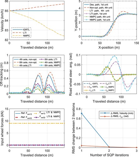
Figure 9. A single-lane-change manoeuvrer. The optimal control of the tractor front axle steering ${\delta }_{11}$ and the dolly front axle steering ${\delta }_{31}$ for following the desired path and off-tracking minimisation of all the units obtained using the LTV-MPC and NMPC (SQP) solution methods. All the other inputs are kept constant, i.e. $F_{\mathrm{xw}12}=F_{\mathrm{xw}12,\mathrm{Ref}}$ and $F_{\mathrm{xw}32}=F_{\mathrm{xw}32,\mathrm{Ref}}$, and the other input forces are zero. ‘Des’ refers to the desired path. The NMPC (SQP) is warm-started with nonzero IGRTL, e.g. a sine steering of ${\delta }_{11,\mathrm{Ref}}$. The NMPC (SQP) converged within a single iteration. The solutions of the LTV-MPC are relatively similar to that of the NMPC (SQP). The non-optimal (non-opt) paths are obtained by simulating the LCV using a sine-steering input of the first axle ${\delta }_{11}$ similar to that obtained by the NMPC, where no optimal control of the other inputs is performed.

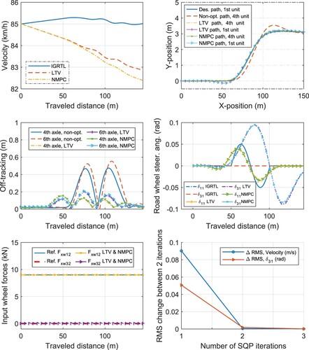
Figure 10. A U-turn manoeuvrer. The optimal control of the tractor front axle steering ${\delta }_{11}$, the dolly front axle steering ${\delta }_{31}$, and propulsion $F_{\mathrm{xw}12}$ and $F_{\mathrm{xw}32}$, whereas the other inputs are kept zero, for desired trajectory-following and off-tracking minimisation of all the units by using the LTV-MPC and NMPC (SQP) solution methods. The second axle of the dolly is equipped with an electric motor. The non-optimal (non-opt) paths are obtained by simulating the LCV using a sine-steering input of the first axle ${\delta }_{11}$ similar to that obtained by the NMPC, where no optimal control of the other inputs is performed.

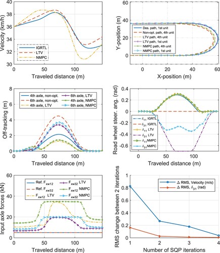
For the U-turn, as shown in Figure 10 the IGRTL is far from the final solution. Therefore, SQP requires at least four sequential iterations to converge, and the LTV-MPC and SQP solutions differ. Moreover, it is observed that the steering of the dolly results in a velocity reduction. The velocity is bounded around the velocity given by the IGRTL by 8% of its value. Therefore, the velocity is kept within the bound by the optimal axles propulsion in the U-turn manoeuvrer. We note that the change of the velocity is not penalised in the cost function. As the result of the optimal control during the U-turn, the dolly steers in the opposite direction compared to the first unit, outward relative to the curve, as illustrated in Figure 11. Furthermore, a controller can be designed to generate a better IGRTL for the U-turn manoeuvrer; this was left for the future studies by the authors.

Figure 11. A-double negotiating the U-turn while the dolly steers outward.

The computation time varies depending on the available computational power and number of discrete steps in the horizon. It takes 0.3 s to solve the quadratic program, if the number of discrete steps is 100 in 100 m horizon. The optimisation solver was Gurobi [61] in the MATLAB platform on a laptop with 2.30 GHz processor. The use of the different solvers on different platforms may reduce the computational time. In addition, on average, generating the Jacobians, i.e. step 2 of Algorithm 1, takes about 20 s. It means that the total computation times of different controllers, in a single-lane change manoeuvrer, are according to the following: LTI-MPC: 0.3 s, LTV-MPC: 0.3 s and NMPC: 40.9 s (after three iterations), assuming that the IGRTL and Jacobians are available in the first iteration.

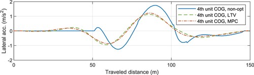
Finally, Figure 12 illustrates the lateral acceleration of the forth vehicle unit of the A-double during high-speed single-lane-change manoeuvrer obtained by different controllers. It can be seen that the lateral acceleration was reduced using LTV and MPC controllers, controlling dolly steering angel, compared to non-steered dolly (non-opt).

Figure 12. Lateral acceleration of the forth vehicle unit COG of the A-double during high-speed single-lane-change manoeuvrer.

7. Conclusion

We proposed a methodology for optimal integrated motion control of LCVs. The vehicle equations of motions were nonlinear and allowed coupled longitudinal and lateral dynamics and combined optimal control of distributed steering, propulsion, and braking in a long prediction horizon. Therefore, the vehicle was able to react optimally prior to reaching a curve in order to increase tracking quality and safety.

We implemented nonlinear and linear MPC for trajectory-following and off-tracking minimisation of an A-double vehicle. We solved the nonlinear MPC problem by sequential quadratic programming, which was unsuitable for the real-time implementation. The RTI approach was not suitable for the real-time implementation either because of the expensive computations needed for linearisation of LCV equations. Alternatively, we converted the nonlinear MPC to a linear time-varying MPC where the linearisation is performed off-line. We showed that the control actions obtained by solving the linear time-varying MPC were relatively close to that generated by sequential quadratic programming if the IGRTL is relatively close to the solution of the nonlinear MPC. Such an IGRTL can either be obtained by performing open-loop simulations or by using a simpler feedback controller than MPC. We also demonstrated that the STL vehicle models are not suitable for such integrated control applications in long prediction horizons.

This work can be extended by defining methods to find ‘good’ linearisation references, including other applications of nonlinear MPC in long combination vehicles such as speed-planning and optimally distributing the propulsion and braking in order to minimise the energy consumption on hilly and curved roads considering the vehicle stability and other road users.

Disclosure statement

No potential conflict of interest was reported by the author(s).

Additional information

Funding

This work was funded by Energimyndigheten [grant number 2015-004985]

Appendices

Appendix 1.

Vehicle modelling

We derived the nonlinear single-track vehicle model in the yaw plane by using the Lagrange equation [19,40,58,68]. A Matlab code for generating the equation of motion of LCVs can be downloaded in [69]. The code and equations are explained in [58] including an experimental validation.

Let ua and sa be binary matrices defining unit axles and steerable axles, respectively, e.g. for the single-track 6-axle vehicle shown in Figure 1: (A1) $\begin{array}{rl}& ua=[1,1;\\ & 1,0;\\ & 1,1;\\ & 1,0],\end{array}$(A1) (A2) $\begin{array}{rl}& sa=[1,0;\\ & 0,0;\\ & 1,0;\\ & 0,0].\end{array}$(A2) Each of the rows of the above matrices provides information about the vehicle units and the their axles; moreover, the total number of rows corresponds to the total number of units $n_{\mathrm{u}}$, e.g. $u{a}_{ij}=1$ and $s{a}_{ij}=1$ means that there is an axle j on unit i that is steerable. The number of columns of the above matrices defines the maximum number of the axles in a unit $n_{\mathrm{a}}$.

The Lagrange equation is given by (A3) $\frac{\mathrm{d}}{\mathrm{d}t}\frac{\mathrm{\partial }T}{\mathrm{\partial }{\dot{q}}_l}-\frac{\mathrm{\partial }T}{\mathrm{\partial }{q}_l}+\frac{\mathrm{\partial }V}{\mathrm{\partial }{q}_l}=Q_l,l=1,\dots ,n_g,$(A3) where T, V, denote the system kinetic and potential energies, $n_g=6$ is the total number of generalised coordinates of the system, and a dot ( $\dot{}$ ) above a variable represents the time derivative. The generalised coordinates q are given by (A4) $q=[X_1,Y_1,{\varphi }_1,{\theta }_1,{\theta }_2,{\theta }_3],$(A4) where $X_1$, $Y_1$ denote the position of the COG of the first unit in global inertia coordinate system, ${\varphi }_1$ and θ denote the global yaw angle of the first unit and articulation angles, respectively. The generalised force $Q_l$ is given by (A5) $Q_l=\sum _{k=1}^{n_{\mathrm{f}}}(F_{\mathrm{X}k}\frac{\mathrm{\partial }{P}_{\mathrm{X}k}}{\mathrm{\partial }{q}_l}+F_{\mathrm{Y}k}\frac{\mathrm{\partial }{P}_{\mathrm{Y}k}}{\mathrm{\partial }{q}_l}),l=1,\dots ,n_g,$(A5) where $n_{\mathrm{f}}$ denotes the total number of force elements, $F_{\mathrm{X}k}$ and $F_{\mathrm{Y}k}$ are their X and Y components and $P_{\mathrm{X}k}$ and $P_{\mathrm{Y}k}$ are their X and Y positions in the global inertia frame.

The potential energy is zero, whereas the kinetic energy is given by (A6) $T=\frac{1}{2}\sum _{i=1}^{n_{\mathrm{u}}}(m_i(v_{\mathrm{X}i}^2+v_{\mathrm{Y}i}^2)+J_i{\dot{\varphi }}_i^2),$(A6) where $m_i$ is the vehicle unit mass, $J_i$ is the vehicle unit yaw moment of inertia, i is the vehicle unit index, ${\varphi }_i$ is the vehicle unit angle in global frame and $v_{\mathrm{X}i}$ and $v_{\mathrm{Y}i}$ are the velocity components of the COG of unit i.

The position of the vehicle units COGs can be determined by using the system kinematics as (A7) $\left[\begin{array}{c}{X}_i\\ Y_i\end{array}\right]=\left[\begin{array}{c}{X}_{i-1}\\ Y_{i-1}\end{array}\right]+\left[\begin{array}{c}{x}_{\mathrm{c}(i-1)2}\cos ({\varphi }_{i-1})-x_{\mathrm{c}i1}\cos ({\varphi }_i)\\ x_{\mathrm{c}(i-1)2}\sin ({\varphi }_{i-1})-x_{\mathrm{c}i1}\sin ({\varphi }_i)\end{array}\right],i=2,\dots ,n_{\mathrm{u}},$(A7) where, (A8) ${\varphi }_i={\varphi }_{i-1}+{\theta }_{i-1},i=2,\dots ,n_{\mathrm{u}},$(A8) and $x_{\mathrm{c}i1}$ and $x_{\mathrm{c}i2}$ are the local positions of the front and rear coupling points. For vehicle dimensions refer to Figure 1 and Table A1. Therefore, the vehicle unit velocities in the global frame are (A9) $v_{\mathrm{X}i}=\frac{\mathrm{d}{X}_i}{\mathrm{d}t},v_{\mathrm{Y}i}=\frac{\mathrm{d}{Y}_i}{\mathrm{d}t}.$(A9) Let M be a matrix for transforming the coordinates in the vehicle unit local frame to the coordinates in the global frame: (A10) $\begin{array}{r}{M}_i=\left[\begin{array}{cc}\cos ({\varphi }_i)& -\sin ({\varphi }_i)\\ \sin ({\varphi }_i)& \cos ({\varphi }_i)\end{array}\right].\end{array}$(A10) Then, the axle global positions are given by (A11) $\left[\begin{array}{c}{X}_{\mathrm{w}ij}\\ Y_{\mathrm{w}ij}\end{array}\right]=\left[\begin{array}{c}{X}_i\\ Y_i\end{array}\right]+M_i\left[\begin{array}{c}{x}_{\mathrm{a}ij}\\ 0\end{array}\right],i=1,\dots ,n_{\mathrm{u}},j=1,\dots ,n_{\mathrm{a}},u{a}_{ij}\ne 0.$(A11) Similarly, the position of the air resistance force is given by (A12) $\left[\begin{array}{c}{X}_{\mathrm{air}}\\ Y_{\mathrm{air}}\end{array}\right]=\left[\begin{array}{c}{X}_1\\ Y_1\end{array}\right]+M_1\left[\begin{array}{c}{x}_{\mathrm{a}11}\\ 0\end{array}\right].$(A12) Therefore, the resulting equation of motion is an implicit system of ODEs in the form (A13) $F(x,\dot{x},u)=0,$(A13) for the state vector $x$ (A14) $x=[X_1,Y_1,{\varphi }_1,v_{\mathrm{X}1},v_{\mathrm{Y}1},\dot{{\varphi }_1},{\theta }_i,\dot{{\theta }_i}],i=1,\dots ,n_{\mathrm{u}}-1,$(A14) and the input vector u that is given by (3(3) $u=[F_{\mathrm{xw}11},F_{\mathrm{xw}12},F_{\mathrm{xw}21},F_{\mathrm{xw}31},F_{\mathrm{xw}32},F_{\mathrm{xw}41},{\delta }_{11},{\delta }_{31}],$(3) ).

However, the state vector defined in (A14(A14) $x=[X_1,Y_1,{\varphi }_1,v_{\mathrm{X}1},v_{\mathrm{Y}1},\dot{{\varphi }_1},{\theta }_i,\dot{{\theta }_i}],i=1,\dots ,n_{\mathrm{u}}-1,$(A14) ) includes velocities $v_{\mathrm{X}1}$ and $v_{\mathrm{Y}1}$ in the global frame. The change of variables from the global frame to the first vehicle unit local frame can be performed using a coordinate transformation described by (A15) $\left[\begin{array}{c}{v}_{\mathrm{x}1}\\ v_{\mathrm{y}1}\end{array}\right]=M_1^{-1}\left[\begin{array}{c}{v}_{\mathrm{X}1}\\ v_{\mathrm{Y}1}\end{array}\right]=\left[\begin{array}{cc}\cos ({\varphi }_1)& \sin ({\varphi }_1)\\ -\sin ({\varphi }_1)& \cos ({\varphi }_1)\end{array}\right]\left[\begin{array}{c}{\dot{X}}_1\\ {\dot{Y}}_1\end{array}\right].$(A15) Therefore, chain rule differentiation must be performed to differentiate the kinetic energy in A3(A3) $\frac{\mathrm{d}}{\mathrm{d}t}\frac{\mathrm{\partial }T}{\mathrm{\partial }{\dot{q}}_l}-\frac{\mathrm{\partial }T}{\mathrm{\partial }{q}_l}+\frac{\mathrm{\partial }V}{\mathrm{\partial }{q}_l}=Q_l,l=1,\dots ,n_g,$(A3) , i.e. (A16) $\begin{array}{rl}\frac{\mathrm{\partial }T}{\mathrm{\partial }{\dot{X}}_1}& =\frac{\mathrm{\partial }T}{\mathrm{\partial }{v}_{\mathrm{x}1}}\frac{\mathrm{\partial }{v}_{\mathrm{x}1}}{\mathrm{\partial }{\dot{X}}_1}+\frac{\mathrm{\partial }T}{\mathrm{\partial }{v}_{\mathrm{y}1}}\frac{\mathrm{\partial }{v}_{\mathrm{y}1}}{\mathrm{\partial }{\dot{X}}_1}=\frac{\mathrm{\partial }T}{\mathrm{\partial }{v}_{\mathrm{x}1}}\cos ({\varphi }_1)-\frac{\mathrm{\partial }T}{\mathrm{\partial }{v}_{\mathrm{y}1}}\sin ({\varphi }_1),\end{array}$(A16) (A17) $\begin{array}{rl}\frac{\mathrm{\partial }T}{\mathrm{\partial }{\dot{Y}}_1}& =\frac{\mathrm{\partial }T}{\mathrm{\partial }{v}_{\mathrm{x}1}}\frac{\mathrm{\partial }{v}_{\mathrm{x}1}}{\mathrm{\partial }{\dot{Y}}_1}+\frac{\mathrm{\partial }T}{\mathrm{\partial }{v}_{\mathrm{y}1}}\frac{\mathrm{\partial }{v}_{\mathrm{y}1}}{\mathrm{\partial }{\dot{Y}}_1}=\frac{\mathrm{\partial }T}{\mathrm{\partial }{v}_{\mathrm{x}1}}\sin ({\varphi }_1)+\frac{\mathrm{\partial }T}{\mathrm{\partial }{v}_{\mathrm{y}1}}\cos ({\varphi }_1),\end{array}$(A17) (A18) $\begin{array}{rl}\frac{\mathrm{\partial }T}{\mathrm{\partial }{\varphi }_1}& =\frac{\mathrm{\partial }T}{\mathrm{\partial }{v}_{\mathrm{x}1}}\frac{\mathrm{\partial }{v}_{\mathrm{x}1}}{\mathrm{\partial }{\varphi }_1}+\frac{\mathrm{\partial }T}{\mathrm{\partial }{v}_{\mathrm{y}1}}\frac{\mathrm{\partial }{v}_{\mathrm{y}1}}{\mathrm{\partial }{\varphi }_1}+\frac{\mathrm{\partial }T}{\mathrm{\partial }g({\varphi }_1)}\frac{\mathrm{\partial }g({\varphi }_1)}{\mathrm{\partial }{\varphi }_1}=\frac{\mathrm{\partial }T}{\mathrm{\partial }{v}_{\mathrm{x}1}}{v}_{\mathrm{y}1}-\frac{\mathrm{\partial }T}{\mathrm{\partial }{v}_{\mathrm{y}1}}{v}_{\mathrm{x}1},\end{array}$(A18) where $\frac{\mathrm{\partial }g({\varphi }_1)}{\mathrm{\partial }{\varphi }_1}=0$.

The new set of states in the first vehicle unit local coordinate system is (A19) $x=[X_1,Y_1,{\varphi }_1,v_{\mathrm{x}1},v_{\mathrm{y}1},\dot{{\varphi }_1},{\theta }_i,\dot{{\theta }_i}],i=1,\dots ,n_{\mathrm{u}}-1.$(A19) Conversion from the time domain to the space domain can be performed by performing the following change of variables that results in the states (2(2) $x=[X_1,Y_1,{\varphi }_1,{\theta }_1,{\theta }_2,{\theta }_3,v_{\mathrm{x}1},v_{\mathrm{y}1},\frac{\mathrm{d}{\varphi }_1}{\mathrm{d}s},\frac{\mathrm{d}{\theta }_1}{\mathrm{d}s},\frac{\mathrm{d}{\theta }_2}{\mathrm{d}s},\frac{\mathrm{d}{\theta }_3}{\mathrm{d}s}],$(2) ) and equations of motion (1(1) $F(x(s),\frac{\mathrm{d}x(s)}{\mathrm{d}s},u(s),s)=0,$(1) ). (A20) $\frac{\mathrm{d}(\cdot )}{\mathrm{d}t}=\frac{\mathrm{d}(\cdot )}{\mathrm{d}s}\frac{\mathrm{d}s}{\mathrm{d}t}\approx v_{\mathrm{x}1}\frac{\mathrm{d}(\cdot )}{\mathrm{d}s},$(A20) and (A21) $\frac{{\mathrm{d}}^2(\cdot )}{\mathrm{d}{t}^2}=\frac{\mathrm{d}}{\mathrm{d}t}\left(\frac{\mathrm{d}(\cdot )}{\mathrm{d}s}\frac{\mathrm{d}s}{\mathrm{d}t}\right)=v_{\mathrm{x}1}^2\frac{{\mathrm{d}}^2(\cdot )}{\mathrm{d}{s}^2}+v_{\mathrm{x}1}\frac{\mathrm{d}{v}_{\mathrm{x}1}}{\mathrm{d}s}\frac{\mathrm{d}(\cdot )}{\mathrm{d}s},$(A21) where $(\cdot )$ represents any variable and where we assumed $\frac{\mathrm{d}s}{\mathrm{d}t}\approx v_{\mathrm{x}1}$.

A.1. tire model

In this section, we removed the axle and unit indices for the sake of brevity. We did not model the tyre longitudinal slip $s_{\mathrm{x}}$. However, the tyre lateral slip is given by (A22) $s_{\mathrm{y}}=\frac{v_{\mathrm{wy}}}{|v_{\mathrm{wx}}|},$(A22) which is the result of the physical derivation of the Brush tyre model [70]. The wheel velocity local components can be calculated according to (A23) $\left[\begin{array}{c}{v}_{\mathrm{wx}}\\ v_{\mathrm{wy}}\end{array}\right]=\left[\begin{array}{cc}\cos (\varphi +\delta )& \sin (\varphi +\delta )\\ -\sin (\varphi +\delta )& \cos (\varphi +\delta )\end{array}\right]\left[\begin{array}{c}\mathrm{d}{X}_{\mathrm{w}}/\mathrm{d}t\\ \mathrm{d}{Y}_{\mathrm{w}}/\mathrm{d}t\end{array}\right].$(A23) The nonlinear tyre model used in this paper is inspired by the Pacejka magic tyre model [71] and was initially reported in project ‘Performance based standards II’ [65]. A modified version of that model [58] reads (A24) $F_{\mathrm{yw}}{|}_{(s_{\mathrm{x}}=0)}=F_{\mathrm{z}}{u}_{\mathrm{y}}\sin \left(C\arctan (\frac{-C_{\mathrm{cy}}}{C{u}_{\mathrm{y}}}\arctan (s_{\mathrm{y}})\right),$(A24) where $F_{\mathrm{z}}$, $C_{\mathrm{cy}}$ and C are the tyre normal force, cornering coefficient and shape factor, respectively. The shape factor is defined as (A25) $C=2(1+\frac{\arcsin (u_2)}{\pi }),$(A25) where $u_2$ is the ratio between the road friction coefficient at a large slip and that at a zero slip, and (A26) $u_{\mathrm{y}}=0.8(1+u_{\mathrm{yg}}\frac{F_{\mathrm{z}}-F_{\mathrm{z}0}}{F_{\mathrm{z}0}}),$(A26) where $F_{\mathrm{z}0}$ is the nominal tyre normal force that in this paper is equal to the axle static load, and $u_{\mathrm{yg}}$ is the maximum lateral force gradient with a value between -0.3 and -0.1. The cornering coefficient $C_{\mathrm{cy}}$ is defined as (A27) $C_{\mathrm{cy}}=C_{\mathrm{cy}0}(1-0.1\frac{F_{\mathrm{z}}-F_{\mathrm{z}0}}{F_{\mathrm{z}0}});$(A27) where $C_{\mathrm{cy}0}$ is the cornering coefficient at the nominal tyre normal force. We tuned the values of the maximum lateral force gradient $u_{\mathrm{yg}}$ and the cornering coefficient $C_{\mathrm{cy}0}$ based on the experimental data [58].

Finally, the combined slip was modelled according to the friction ellipse model [58,70,71] according to (A28) $F_{\mathrm{yw}}=\sqrt{1-{\left(\frac{F_{\mathrm{xw}}}{e\mu F_{\mathrm{z}}}\right)}^2}{F}_{\mathrm{yw}}{|}_{(s_{\mathrm{x}}=0)}$(A28) where e is a scaling factor defining the shape of the ellipse; e.g. if e = 1 the model is a friction circle.

Finally, the tyre forces in the global frame can be defined as $\left[\begin{array}{c}{F}_{\mathrm{X}}\\ F_{\mathrm{Y}}\end{array}\right]=\left[\begin{array}{c}\cos (\varphi +\delta )-\sin (\varphi +\delta )\\ \sin (\varphi +\delta )\cos (\varphi +\delta )\end{array}\right]\left[\begin{array}{c}{F}_{\mathrm{xw}}\\ F_{\mathrm{yw}}\end{array}\right],$

A.2. Gravitational force, rolling and air resistance forces

Assuming that the road pitch and banking angles remain constant within a unit length, the gravitational force acting on the COG of unit i is given by (A29) $\begin{array}{rl}{F}_{\mathrm{gx}i}& =m_{i}g\sin ({\lambda }_{\mathrm{p}i}),\end{array}$(A29) (A30) $\begin{array}{rl}{F}_{\mathrm{gy}i}& =m_{i}g\sin ({\lambda }_{\mathrm{b}i}),\end{array}$(A30) where g is gravitational acceleration, the road pitch angle ${\lambda }_{\mathrm{p}i}$ is positive downhill in front of the vehicle unit, and the road banking angle ${\lambda }_{\mathrm{b}i}$ is positive downhill at the left side of the vehicle unit.

The gravitational forces acting on units COGs in the global frame are given by (A31) $\left[\begin{array}{c}{F}_{\mathrm{gX}i}\\ F_{\mathrm{gY}i}\end{array}\right]=\left[\begin{array}{cc}\cos ({\varphi }_{\mathrm{r}i})& -\sin ({\varphi }_{\mathrm{r}i})\\ \sin ({\varphi }_{\mathrm{r}i})& \cos ({\varphi }_{\mathrm{r}i})\end{array}\right]\left[\begin{array}{c}{F}_{\mathrm{gx}i}\\ F_{\mathrm{gy}i}\end{array}\right],$(A31) where ${\varphi }_{\mathrm{r}i}$ is the road yaw angle in the global frame. However, we assumed ${\varphi }_{\mathrm{r}i}={\varphi }_i$.

The rolling resistance forces $F_{\mathrm{wRR}}$ are defined as (A32) $F_{\mathrm{wRR}}=-f_{\mathrm{r}}{F}_{\mathrm{z}}\frac{v_{\mathrm{x}1}}{|v_{\mathrm{x}1}|},$(A32) and in the global coordinates are $\left[\begin{array}{c}{F}_{\mathrm{XRR}}\\ F_{\mathrm{YRR}}\end{array}\right]=\left[\begin{array}{c}\cos ({\varphi }_i+\delta )-\sin ({\varphi }_i+\delta )\\ \sin ({\varphi }_i+\delta )\cos ({\varphi }_i+\delta )\end{array}\right]\left[\begin{array}{c}{F}_{\mathrm{wRR}}\\ 0\end{array}\right],$ where $f_{\mathrm{r}}$ is the rolling resistance coefficient.

Finally, the air resistance force is given by (A33) $\begin{array}{rl}{F}_{\mathrm{x}air}& =-0.5A_{\mathrm{f}}{c}_{\mathrm{d}}{\rho }_{\mathrm{a}}{v}_{\mathrm{x}1}^2\frac{v_{\mathrm{x}1}}{|v_{\mathrm{x}1}|},\end{array}$(A33) (A34) $\begin{array}{rl}\left[\begin{array}{c}{F}_{\mathrm{Xair}}\\ F_{\mathrm{Yair}}\end{array}\right]& =\left[\begin{array}{cc}\cos ({\varphi }_1)& -\sin ({\varphi }_1)\\ \sin ({\varphi }_1)& \cos ({\varphi }_1)\end{array}\right]\left[\begin{array}{c}{F}_{\mathrm{x}air}\\ 0\end{array}\right],\end{array}$(A34) where $A_{\mathrm{f}}$, $c_{\mathrm{d}}$ and ${\rho }_{\mathrm{a}}$ are the vehicle front area, air drag coefficient and air density, respectively.

Appendix 2.

Vehicle parameters

In this paper, g = 9.81 $\frac{\mathrm{m}}{{\mathrm{s}}^2}$, e = 1, $A_{\mathrm{f}}{c}_{\mathrm{d}}{\rho }_{\mathrm{a}}$ = 9.9840 $\frac{\mathrm{N}{\mathrm{s}}^2}{{\mathrm{m}}^2}$, $f_{\mathrm{r}}$ = 0.008, $u_2$ = 0.8; and for each of the tires of the steered axles: $u_{\mathrm{yg}}$ = -0.168, $C_{\mathrm{cy}0}$ =5.33, and for un-steered axles: $u_{\mathrm{yg}}$ = -0.1, $C_{\mathrm{cy}0}$ =12.38. Other parameters are shown in Table A1.

Table A1. Vehicle unit and axle parameters.

Parameter	Unit 1	Unit 2	Unit 3	Unit 4
m (kg)	10,250	22,000	3700	24,300
J (kg m${}^2$)	$0.4671\times {10}^5$	$1.6291\times {10}^5$	$0.0708\times {10}^5$	$3.0895\times {10}^5$
$x_{\mathrm{a}}$ (m)	[1.4992, −2.5858]	[−2.5687, 0]	[0.5499, −1.4501]	[−2.4778, 0]
$x_c$ (m)	[0, −2.2008]	[5.1313, −5.3187]	[3.8999, −0.4001]	[5.4222, 0]
$n_{\mathrm{ta}}$${}^{\ast }$	[2, 8]	[6, 0]	[2, 2]	[6, 0]
μ	[1, 1]	[1, 0]	[1, 1]	[1, 0]

Note: The first vehicle unit has two axles and the other units have a single axle. ‘0’ means that either the quantity is not relevant or the axle does not exist.

${}^{\ast }$ $n_{\mathrm{ta}}$ denotes the number of tires per axle.

Appendix 3.

Abbreviations

Abbreviations used in this paper are provided in Table A2.

Table A2. List of abbreviations.

Abbreviation	Meaning	Abbreviation	Meaning
COG	Centre of gravity	NMPC	Nonlinear model predictive control
DAE	Differential algebraic equation	ODE	Ordinary differential equation
IGRTL	Initial guess of the reference trajectories used for linearisation	QP	Quadratic programme
LCV	Long combination vehicle	RMS	Root mean square
LTI	Linear time-invariant	RTIs	Real-time iterations
LTV-MPC	Linear time-varying model predictive control	SQP	Sequential quadratic programming
MPC	Model predictive control	STL	Single-track linear

References

- European Commission. Road transport: reducing co 2 emissions from vehicles; 2016. Available from: https://ec.europa.eu/clima/policies/transport/vehicles_en.
- Rodrigues VS, Piecyk M, Mason R, et al. The longer and heavier vehicle debate: a review of empirical evidence from Germany. Trans Res Part D: Trans Environ. 2015;40:114–131. doi:10.1016/j.trd.2015.08.003
- Woodrooffe JH, Ash L. Economic efficiency of long combination transport vehicles in Alberta. Edmonton: Woodrooffe & Associates; 2001.
- Ghandriz T, Jacobson B, Laine L, et al. Impact of automated driving systems on road freight transport and electrified propulsion of heavy vehicles. Trans Res Part C: Emerg Technol. 2020;115:102610. doi:10.1016/j.trc.2020.102610
- Ghandriz T, Jacobson B, Laine L, et al. Optimization data on total cost of ownership for conventional and battery electric heavy vehicles driven by humans and by automated driving systems. Data Br. 2020;30:105566. doi:10.1016/j.dib.2020.105566
- Kockum S, Örtlund R, Ekfjorden A, et al. Volvo trucks safety report; 2017. Available from: https://www.volvogroup.com/content/dam/volvo/volvo-group/markets/global/en-en/about-us/traffic-safety/Safety-report-2017.pdf.
- European Commission. Traffic safety basic facts 2018 – heavy goods vehicles and buses; 2018. Available from: https://ec.europa.eu/transport/road_safety/sites/roadsafety/files/pdf/statistics/dacota/bfs20xx_hgvs.pdf.
- Christidis P, Leduc G. Longer and heavier vehicles for freight transport. JRC Eur Comm. 2009;1–40. Available from: http://www.eurosfaire.prd.fr/7pc/doc/1245745030_lhv_trucks_jrc52005.pdf.
- Grislis A. Longer combination vehicles and road safety. Transport. 2010;25(3):336–343. doi:10.3846/transport.2010.41
- Lemp JD, Kockelman KM, Unnikrishnan A. Analysis of large truck crash severity using heteroskedastic ordered probit models. Accid Anal Prev. 2011;43(1):370–380. doi:10.1016/j.aap.2010.09.006
- SAE standard. Taxonomy and definitions for terms related to on-road motor vehicle automated driving systems. Vol. 3016, SAE Standard J. 2016. p. 1–16.
- Alessandrini A, Campagna A, Delle Site P, et al. Automated vehicles and the rethinking of mobility and cities. Transp Res Proc. 2015;5:145–160. doi:10.1016/j.trpro.2015.01.002
- Anderson JM, Nidhi K, Stanley KD, et al. Autonomous vehicle technology: a guide for policymakers. Santa Monica (CA): Rand Corporation; 2014.
- Chan CY. Advancements, prospects, and impacts of automated driving systems. Int J Transp Sci Technol. 2017;6(3):208–216. doi:10.1016/j.ijtst.2017.07.008
- Kalra N, Paddock SM. Driving to safety: how many miles of driving would it take to demonstrate autonomous vehicle reliability?. Transp Res Part A Policy Pract. 2016;94:182–193. doi:10.1016/j.tra.2016.09.010
- Trigell AS, Rothhämel M, Pauwelussen J, et al. Advanced vehicle dynamics of heavy trucks with the perspective of road safety. Veh Syst Dyn. 2017;55(10):1572–1617.
- Paden B, Čáp M, Yong SZ, et al. A survey of motion planning and control techniques for self-driving urban vehicles. IEEE Trans Intell Veh. 2016;1(1):33–55.
- van Duijkeren N, Keviczky T, Nilsson P, et al. Real-time nmpc for semi-automated highway driving of long heavy vehicle combinations. IFAC-PapersOnLine. 2015;48(23):39–46.
- Luijten M. Lateral dynamic behaviour of articulated commercial vehicles. Eindhoven University of Technology; 2010. Available from: http://www.mate.tue.nl/mate/pdfs/12050.pdf.
- ISO14791 I. Road vehicles-heavy commercial vehicle combinations and articulated buses-lateral stability test methods. Tech. rep; 2002.
- He Y, Islam MM, Webster TD. An integrated design method for articulated heavy vehicles with active trailer steering systems. SAE Int J Passeng Cars-Mech Syst. 2010;3(2010-01-0092):158–174. doi:10.4271/2010-01-0092
- Islam MM, Ding X, He Y. A closed-loop dynamic simulation-based design method for articulated heavy vehicles with active trailer steering systems. Veh Syst Dyn. 2012;50(5):675–697. doi:10.1080/00423114.2011.622904
- Diehl M, Findeisen R, Allgöwer F, et al. Nominal stability of real-time iteration scheme for nonlinear model predictive control. IEE Proc Control Theory Appl. 2005;152(3):296–308. doi:10.1049/ip-cta:20040008
- Gros S, Zanon M, Quirynen R, et al. From linear to nonlinear mpc: bridging the gap via the real-time iteration. Int J Control. 2020;93(1):62–80.
- Falcone P, Tseng HE, Asgari J, et al. Integrated braking and steering model predictive control approach in autonomous vehicles. IFAC Proc Vol. 2007;40(10):273–278.
- Falcone P, Tufo M, Borrelli F, et al. A linear time varying model predictive control approach to the integrated vehicle dynamics control problem in autonomous systems. In: 2007 46th IEEE Conference on Decision and Control; IEEE; 2007. p. 2980–2985.
- Falcone P, Borrelli F, Tseng HE, et al. Linear time-varying model predictive control and its application to active steering systems: stability analysis and experimental validation. Int J Robust Nonlinear Control IFAC-Affiliated J. 2008;18(8):862–875.
- Yuan H, Gao Y, Gordon TJ. Vehicle optimal road departure prevention via model predictive control. Proc Inst Mech Eng Part D: J Aut Eng. 2017;231(7):952–962. doi:10.1177/0954407017701286
- Zhang Y, Khajepour A, Ataei M. A universal and reconfigurable stability control methodology for articulated vehicles with any configurations. IEEE Trans Veh Technol. 2020;69(4):3748–3759. doi:10.1109/TVT.2020.2973082
- Kraaijenhagen B, van der Zweep C, Lischke A, et al. Aerodynamic and flexible trucks for next generation of long distance road transport (aeroflex). International Forum For Road Transport technology (IFRTT); 2018. Available from: https://elib.dlr.de/122283/.
- Deng W, Kang X. Parametric study on vehicle-trailer dynamics for stability control. SAE Trans. 2003;112:1411–1419.
- Hac A, Fulk D, Chen H. Stability and control considerations of vehicle-trailer combination. SAE Int J Passeng Cars-Mech Syst. 2008;1(2008-01-1228):925–937. doi:10.4271/2008-01-1228
- Rouchon P, Fliess M, Lévine J, et al. Flatness, motion planning and trailer systems. In: Proceedings of 32nd IEEE Conference on Decision and Control; IEEE; 1993. p. 2700–2705. Available from: https://doi.org/10.1109/CDC.1993.325686
- Van de Molengraft-Luijten M, Besselink IJ, Verschuren R, et al. Analysis of the lateral dynamic behaviour of articulated commercial vehicles. Veh Syst Dyn. 2012;50(sup1):169–189. doi:10.1080/00423114.2012.676650
- Sampson DJM. Active roll control of articulated heavy vehicles [dissertation]. University of Cambridge, UK; 2000. Available from: http://www.sampson.id.au/david/work/phd.pdf.
- Morrison G, Cebon D. Combined emergency braking and turning of articulated heavy vehicles. Veh Syst Dyn. 2017;55(5):725–749. doi:10.1080/00423114.2016.1278077
- Wang Q, He Y. A study on single lane-change manoeuvres for determining rearward amplification of multi-trailer articulated heavy vehicles with active trailer steering systems. Veh Syst Dyn. 2016;54(1):102–123. doi:10.1080/00423114.2015.1123280
- Islam MM, He Y, Zhu S, et al. A comparative study of multi-trailer articulated heavy-vehicle models. Proc Inst Mech Eng Part D: J Aut Eng. 2015;229(9):1200–1228. doi:10.1177/0954407014557053
- Sundström P, Jacobson B, Laine L. Vectorized single-track model in modelica for articulated vehicles with arbitrary number of units and axles. In: Modelica conference 2014, Lund: Sweden; 2014. Available from: http://publications.lib.chalmers.se/records/fulltext/190501/local_190501.pdf.
- Nilsson P, Tagesson K. Single-track models of an a-double heavy vehicle combination. Chalmers University of Technology; 2014. Available from: http://publications.lib.chalmers.se/records/fulltext/192958/local_192958.pdf.
- Kharrazi S, Lidberg M, Roebuck R, et al. Implementation of active steering on longer combination vehicles for enhanced lateral performance. Veh Syst Dyn. 2012;50(12):1949–1970. doi:10.1080/00423114.2012.708422
- Kharrazi S, Lidberg M, Fredriksson J. A generic controller for improving lateral performance of heavy vehicle combinations. Proc Inst Mech Eng Part D: J Aut Eng. 2013;227(5):619–642. doi:10.1177/0954407012454616
- Roebuck R, Odhams A, Tagesson K, et al. Implementation of trailer steering control on a multi-unit vehicle at high speeds. J Dyn Syst Meas Control. 2014;136(2):021016. doi:10.1115/1.4025815
- Rangavajhula K, Tsao HSJ. Active trailer steering control of an articulated system with a tractor and three full trailers for tractor-track following. Int J Heavy Veh Syst. 2007;14(3):271–293. doi:10.1504/IJHVS.2007.015604
- Ghilardelli F, Lini G, Piazzi A. Path generation using η4-splines for a truck and trailer vehicle. IEEE Trans Autom Sci Eng. 2013;11(1):187–203. 10.1109/TASE.2013.2266962
- Nilsson P, Laine L, Jacobson B, et al. Driver model based automated driving of long vehicle combinations in emulated highway traffic. In: 2015 IEEE 18th International Conference on Intelligent Transportation Systems; IEEE; 2015. p. 361–368. Available from: https://doi.org/10.1109/ITSC.2015.68
- Nilsson P, Laine L, Van Duijkeren N, et al. Automated highway lane changes of long vehicle combinations: A specific comparison between driver model based control and non-linear model predictive control. In: 2015 International Symposium on Innovations in Intelligent SysTems and Applications (INISTA); IEEE; 2015. p. 1–8. https://doi.org/10.1109/INISTA.2015.7276790
- Kati MS. On robust steering based lateral control of longer and heavier commercial vehicles. Chalmers University of Technology; 2018. Available from: https://research.chalmers.se/en/publication/507376.
- Fancher P, Winkler C, Ervin R, et al. Using braking to control the lateral motions of full trailers. Veh Syst Dyn. 1998;29(S1):462–478. doi:10.1080/00423119808969579
- MacAdam C, Hagan M. A simple differential brake control algorithm for attenuating rearward amplification in doubles and triples combination vehicles. Veh Syst Dyn. 2002;37(sup1):234–245. doi:10.1080/00423114.2002.11666235
- Bin Y, Shim T, Feng N, et al. Path tracking control for backing-up tractor-trailer system via model predictive control. In: 2012 24th Chinese Control and Decision Conference (CCDC); IEEE; 2012. p. 198–203. https://doi.org/10.1109/CCDC.2012.6242930
- Gutjahr B, Gröll L, Werling M. Lateral vehicle trajectory optimization using constrained linear time-varying mpc. IEEE Trans Intell Transp Syst. 2016;18(6):1586–1595. doi:10.1109/TITS.2016.2614705
- Lima PF. Optimization-based motion planning and model predictive control for autonomous driving: With experimental evaluation on a heavy-duty construction truck [dissertation]. KTH Royal Institute of Technology; 2018. Available from: https://www.diva-portal.org/smash/record.jsf?pid=diva2%3A1241535&dswid=2778.
- Sastry S. Nonlinear systems: analysis, stability, and control. Springer Science & Business Media; 2013.
- Lima PF, Mårtensson J, Wahlberg B. Stability conditions for linear time-varying model predictive control in autonomous driving. In: 2017 IEEE 56th Annual Conference on Decision and Control (CDC); IEEE; 2017. p. 2775–2782. Available from: https://doi.org/10.1109/CDC.2017.8264062
- Bock HG, Diehl M, Kostina E, et al. Constrained optimal feedback control of systems governed by large differential algebraic equations. In: Real-time pde-constrained optimization. SIAM; 2007. p. 3–24.
- Bock HG, Diehl M, Kühl P, et al. Numerical methods for efficient and fast nonlinear model predictive control. In: Assessment and future directions of nonlinear model predictive control. Springer; 2007. p. 163–179. Available from: https://doi.org/10.1007/978-3-540-72699-9_13
- Ghandriz T, Jacobson B, Nilsson P, et al. Computationally efficient nonlinear one- and two-track models for multitrailer road vehicles. IEEE Access. 2020;1–22. doi:10.1109/ACCESS.2020.3037035
- Ghandriz T, Jacobson B, Murgovski N, et al. Real-time predictive energy management of hybrid electric heavy vehicles by sequential programming. IEEE Trans Veh Technol. 2021;70(5):4113–4128. doi:10.1109/TVT.2021.3069414
- Andersson JA, Gillis J, Horn G, et al. Casadi: a software framework for nonlinear optimization and optimal control. Math Program Comput. 2019;11(1):1–36.
- Gurobi Optimization L. Gurobi optimizer reference manual ; 2020. Available from: http://www.gurobi.com.
- Nocedal J, Wright S. Numerical optimization. Springer Science & Business Media; 2006.
- Eich-Soellner E, Führer C. Numerical methods in multibody dynamics. Vol. 45. Stuttgart: Teubner; 1998.
- Zhu M, Chen H, Xiong G. A model predictive speed tracking control approach for autonomous ground vehicles. Mech Syst Signal Process. 2017;87:138–152.
- Performance Based Standards II project [https://www.chalmers.se/en/projects/Pages/Performance-Based-Standards-II.aspx]; 2018.
- Kharrazi S, Karlsson R, Sandin J, et al. Performance based standards for high capacity transports in Sweden, FIFFI project 2013-03881, report 1: Review of existing regulations and literature. 2015. Available from: http://www.diva-portal.org/smash/record.jsf?pid=diva2%3A1168835&dswid=-5021.
- Ghandriz T. Transportation mission-based optimization of heavy combination road vehicles and distributed propulsion, including predictive energy and motion control Doctoral thesis, no 4882. Chalmers University of Technology; 2020. Available from: https://research.chalmers.se/en/publication/520358.
- Shabana AA. Dynamics of multibody systems. Cambridge: Cambridge University Press; 2003.
- Ghandriz T. Multitrailer vehicle simulation: Generation and integration of differential equations ; 2020. Available from: https://doi.org/10.5281/zenodo.4248263
- Jacobson B. Vehicle dynamics compendium. Chalmers University of Technology; 2019. Available from: https://research.chalmers.se/en/publication/513850.
- Pacejka H. Tire and vehicle dynamics. Elsevier; 2005.