A low computation-cost locomotion control for underwater snake robot based on Monte Carlo model predictive control and curvature derivative control

ABSTRACT

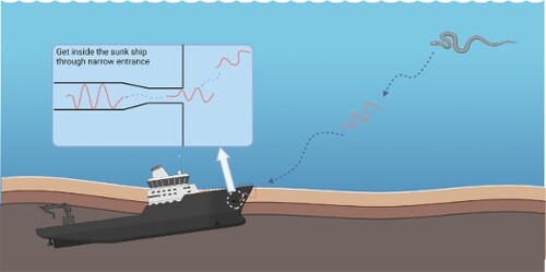
This work studies the application of a sample-based model Monte Carlo Model Predictive Control (MCMPC) to address discontinuous events, such as collisions. The inclusion of contact dynamics in the prediction steps of MCMPC renders it advantageous for the operation of underwater snake robots in restricted environments during rescue missions. The Curvature Derivative Control (CDC) method is employed for the purpose of controlling the joints, with the exception of the head joint. The snake robot body demonstrates adaptability to various environments with the assistance of the CDC. Results obtained from the simulation demonstrate that the snake robot is capable of autonomously navigating from its beginning position outside the region to a pipe as the entrance in order to get inside. The robot successfully traverses through various internal structures within the pipe and ultimately reaches the intended destination, guided by a predetermined cost function of MCMPC. By using the capabilities of CUDA GPU parallel computing, the computational time is substantially lowered.

GRAPHICAL ABSTRACT

KEYWORDS:

• Snake robot
• Monte Carlo method
• model predictive control

1. Introduction

Nature and wild creatures are a great source of inspiration for researchers and engineers. The snake robot, which draws inspiration from nature, was selected because it has a large number of degrees of freedom (DOFs), allowing it to perform a variety of duties, including search and rescue operations. These working settings are typically characterized by severe environmental danger as well as operational space limits, such as inner pipes and sunken ships, that may be too small and unreachable for humans and regular-sized robots. Hirose's [1] work of the first snake robot marked the beginning of the study on snake robots. Although the snake robot's redundancy might be useful for optimization tasks, it also makes control challenging.

Due to the complicated, constrained, and hazardous underwater working environment, the necessity for underwater exploration and observation has grown significantly in recent years. The underwater snake robot is more adaptable, more capable of access and intervention than traditional underwater robots like autonomous underwater vehicles (AUVs) and remotely operated underwater vehicles (ROVs) [2–6]. First proposed in [2], the dynamic model of an underwater snake robot incorporates hydrodynamics with both linear and nonlinear drag forces, additional mass force, and the influence of the ocean current [6]. However, the model is only examined in two dimensions and is predicated on the idea that the robot is neutrally buoyant, meaning that gravity and buoyancy force cancel each other out.

The benefits of the snake body's unique structure make it better suited for search and rescue operations, particularly in confined areas [7]. Certain impediments in a congested environment could be hard or pointless for snake robots to navigate. Using the contact force or propulsion force between the snake links and the barriers, the snake has been observed to move forward by the help of contact forces in such kind of scenario [5,8]. These types of movement are described as obstacle-aided movement. The snake robot would provide other types of mobility in other difficult terrain and restricted environments [7].

1.1. Locomotion patterns of snake robot

Snake robots are capable of functioning in an extensive range of environments, including subterranean, rocky, and confined spaces, among others. The snake exhibits a variety of gait patterns in response to environmental alterations. The snake robot's locomotion in the underwater environment is governed by a lateral undulation [5,9].

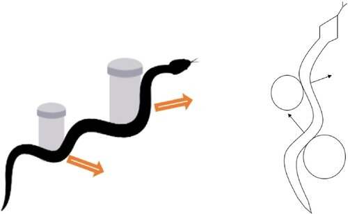
The slender body structure enables snakes to traverse extremely complex and confined spaces while avoiding environmental interference. Snakes exhibit environmental adaptation through the utilization of diverse body shapes while traversing different locations, including maneuvering through pipelines and navigating obstacles [10,11]. Snakes propel themselves forward more efficiently in nature by utilizing external propulsion forces generated by contact with mass-specific objects, such as boulders and stones. This type of reaction force is typical at the interfaces where the link and the obstruction make contact. As illustrated in Figure 1, the propulsion forces of the snake robot are generated through contact with the obstacles, which aid in its more efficient forward motion. The initial proposal to apply the reaction force across obstructions in the construction of a wheeled snake robot appeared in [12]. As obstacle-aided dynamics of the snake robot, this method of generating contact force and friction by pressing the snake body against the obstacles was described in [13]. The authors of [8] proposed a hybrid dynamic model for a planer robot's contact with obstacles. The friction between the obstacle and the snake body was simulated using a coulomb friction model, while the contact force was calculated as a linear complementarity problem(LCP).

Figure 1. A simple schematic of the obstacle-aided locomotion.

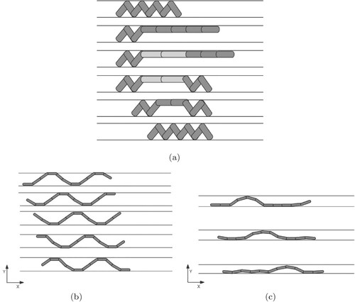
When traversing a confined space, such as a pipe, the snake robot's links will utilize friction to propel itself forward due to the contact pressure between the pipe's surfaces and the robot. The mentioned self-locking phenomenon is implemented in [14] for concertina movement optimization during ascent through a vertical conduit and actuator torque. The result demonstrates that the quantity of connections in contact with the surface also exerts an impact. A greater number of contact linkages requires less torque. Shapiro et al. [15] introduced a frictional compliance model to enable the snake robot to maintain stability and prevent slippage while ascending between two walls. This was accomplished by utilizing the frictional contact produced by the robot's body and the surrounding environment. The author demonstrates in [16] how a change in pipe diameter during pipe inspection operations affects the inspection performance of pipe robots. A sinusoidal gait pattern is intentionally programmed into the snake robot to facilitate movement control and enable it to adapt to its various surroundings. Ivan et al. [17] introduced a travelling wave resembling a trapezium to describe the motion of a snake robot through a pipe. In contrast to the concertina locomotion employed by snakes to traverse confined spaces, rectilinear locomotion is achieved when traversing extremely narrow environments. Figure 2 merely illustrates the concertina locomotion and rectilinear locomotion executed by the snake robot as it traverses the pipe.

Figure 2. Various kinds of locomotion for the snake to move through narrow space. (a) Concertina locomotion of snake (b) Trapezium-like travelling wave locomotion (c) Rectilinear locomotion of the snake.

1.2. Control method of snake robot

Previous research has established a predetermined gait pattern for underwater snake robots, allowing the robot to simply execute the intended locomotion throughout its operations [18]. However, in order to adapt to the various environment and the extreme complexity and unpredictability of the explored space, the snake robot must produce a variety of movements. In recent times, model predictive control (MPC) has been implemented in snake robot control. MPC is an optimal control method that applies the optimal input to the system after solving a finite-horizon optimization problem. In [19], Economic model predictive control (EMPC) is utilized for the control of a simplified snake robot model, The results demonstrate that the snake robot generates a variety of patterns without requiring a predefined gait pattern, and Economic MPC shows better performance in energy consumption and forward moving speed. Evan et al. [20] show the efficacy of using Economic MPC for obstacle-aided snake locomotion. A continuous compliant contact model was proposed. The resulting gait patterns were undulatory and the snake robot used the anisotropic ground friction to move forward. Nevertheless, the simulations require between 5 and 200 s to compute each optimal input, and no effort was made to reduce this duration.

Different from the gradient-based MPC, sample-based MPC does not require gradient information so that discontinuities can be incorporated directly into the MPC prediction steps. Monte Carlo model predictive control (MCMPC), a type of sample-based MPC, was utilized for the underwater snake robot [21]. By introducing the contact dynamics into the system, we demonstrate that the robot is capable of traversing environments with multiple obstacles and generates obstacle-aided locomotion. MATLAB 2021b was used for simulation and each control cycle requires an extremely long computation time. Consequently, CUDA, which uses GPU parallel computing is utilized to reduce time consumption.

The objective of this study is to examine the impact of incorporating MCMPC and CDC on the locomotion of snake robots under various scenarios. This work makes a contribution by conducting assessments on the advantages of employing proposed control methods as control systems for the snake robot. The utilization of these control approaches enables the snake robot to navigate through diverse pipe systems characterized by varying and changing widths. This study introduces the evaluation of the effectiveness of the suggested control approach through the assessment of computation time and generated optimal locomotion of snake robot. This is achieved by including contact dynamics into the prediction step of MCMPC.

The paper is organized as follows, the dynamic model of the snake robot and the hydrodynamics incorporated into the system are illustrated in Section 2. A brief introduction of the primary procedure of how MCMPC works is introduced in Section 3. This study also give a brief introduce of Curvature Derivative Control (CDC) and highlights the benefits of combining these two control methods. The simulation environment and results are presented in Section 4. Subsequently, in Section 5, the conclusions of the study and future research objectives are outlined.

2. Dynamic model of snake robot

This section presents the complex model of the underwater snake robot's system dynamics. Initially, the mathematical model of the snake robot, which incorporates various hydrodynamics, is presented in [2]. Following this, a transformation is applied to the dynamic model to make it CUDA-compatible for utilization in GPU parallel computation. In conclusion, the model of the associated contact force and contact detection are presented. Table 1 shows the related definitions of the mathematical symbols for this study.

Table 1. Definations of mathematical symbols.

Symbol	Description
$n_{\mathrm{link}}$	The total number of links of the snake robot
l	The half length of the link, total length is thus $2l$
m	The mass of each link
${\varphi }_i$	The ith joint angle
${\theta }_i$	The ith link angle
$x_i,y_i$	Center of mass of the ith link in global coordinate
$p_x,p_y$	Center of mass of the snake robot in global coordinate
${\lambda }_1$	Coefficient of the added mass force
${\lambda }_2,{\lambda }_3$	Coefficients of the drag force
${\alpha }_i$	The direction parameter determines the side of contact with the pipe
$k_{\mathrm{msd}},d_{\mathrm{msd}}$	The spring and damping coefficients
${\text{R}}_{{\text{L}}_{\text{i}}}^{\text{global}}$	The rotation matrix from the link frame to the global frame

2.1. Kinematics of the underwater snake robot

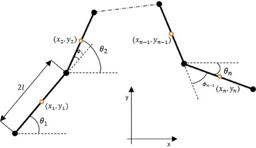
The complex dynamic model of the underwater snake robot is introduced in [6]. Figure 3 shows the structure of the robot which contains $n_{\mathrm{link}}$ links, and the distance between the endpoint and the center of mass (CM) of each link $i\in 1,\dots ,n_{\mathrm{link}}$ is l so that the total length of one link is $2l$. The mass of each link is maintained the same at m. The CM position is utilized to represent the x-y coordinates of each link as $x_i$ and $y_i$ in the global frame. The CM of the whole robot ${\mathrm{P}}_{\mathrm{CM}}\in {\mathbb{R}}^2$ is given by (1) $\begin{array}{r}{\mathrm{P}}_{\mathrm{CM}}=\left[\begin{array}{c}{p}_x\\ p_y\end{array}\right]=\left[\begin{array}{c}\frac{1}{n_{\mathrm{link}}m}\sum _{i=1}^{n_{\mathrm{link}}}m{x}_i\\ \frac{1}{n_{\mathrm{link}}m}\sum _{i=1}^{n_{\mathrm{link}}}m{y}_i\end{array}\right],\end{array}$(1) Moreover, the state variables are specified as $\mathbf{x}=[{\theta }^T,{\mathrm{P}}_{\mathrm{CM}}^T,{\dot{\theta }}^T,{\dot{\mathrm{P}}}_{\mathrm{CM}}^T{]}^T\in {\mathbb{R}}^{2n+4}$ where $\theta \in {\mathbb{R}}^n$ represents the link angle which is defined as the angle formed by each link with respect to the global x-axis. This 2-dimensional model is proposed under the assumption that the snake robot moves in a virtual horizontal and flat plane, and the whole snake body is fully submerged. The robot has $n_{\mathrm{link}}+2$ degrees of freedom which contain the x−y position in the plane, $n_{\mathrm{link}}-1$ joint coordinates, and the orientation, respectively.

Figure 3. Kinematic model of the underwater snake robot.

Hydrodynamics are represented in a simplistic manner in the modelling due to the complexity [2]. The total hydrodynamic forces include ocean current, linear and nonlinear drag forces, and added mass forces, as these types of forces significantly contribute to the propulsion of underwater movements [22]. Several assumptions regarding the dynamic model of the underwater snake robot are presented.

• The fluid is viscid, incompressible, and irrotational in the inertia frame.

• The gravity and the buoyancy cancels each other.

• The current expressed in the inertia frame is contact and irrotational.

It is presumed that the velocity on any part of the link is represented by the relative velocity of the center of mass of each link. The Reynolds number of the surrounding environment estimates to be between ${10}^4$ to ${10}^5$. The representation of the fluid forces acting on each link is shown as (2) $\begin{array}{r}\left[\begin{array}{c}{\mathbf{f}}_{\mathbf{x}}\\ {\mathbf{f}}_{\mathbf{y}}\end{array}\right]=\left[\begin{array}{c}{\mathbf{f}}_{{\mathbf{A}}_{\mathbf{x}}}\\ {\mathbf{f}}_{{\mathbf{A}}_{\mathbf{y}}}\end{array}\right]+\left[\begin{array}{c}{\mathbf{f}}_{{\mathbf{D}}_{\mathbf{x}}}^{\mathbf{I}}\\ {\mathbf{f}}_{{\mathbf{D}}_{\mathbf{y}}}^{\mathbf{I}}\end{array}\right]+\left[\begin{array}{c}{\mathbf{f}}_{{\mathbf{D}}_{\mathbf{x}}}^{\mathbf{II}}\\ {\mathbf{f}}_{{\mathbf{D}}_{\mathbf{y}}}^{\mathbf{II}}\end{array}\right]\end{array}$(2) where ${\mathbf{f}}_{{\mathbf{A}}_{\mathbf{x}}},{\mathbf{f}}_{{\mathbf{A}}_{\mathbf{y}}}$ represents the added mass force. The vector ${\mathbf{f}}_{{\mathbf{D}}_{\mathbf{x}}}^{\mathbf{I}},{\mathbf{f}}_{{\mathbf{D}}_{\mathbf{y}}}^{\mathbf{I}}$ and ${\mathbf{f}}_{{\mathbf{D}}_{\mathbf{x}}}^{\mathbf{II}},{\mathbf{f}}_{{\mathbf{D}}_{\mathbf{y}}}^{\mathbf{II}}$ show the linear and nonlinear drag forces, respectively. As introduced in [2], the added mass force is expressed as (3) $\begin{array}{rl}\left[\begin{array}{c}{\mathbf{f}}_{{\mathbf{A}}_{\mathbf{x}}}\\ {\mathbf{f}}_{{\mathbf{A}}_{\mathbf{y}}}\end{array}\right]& =-\left[\begin{array}{cc}{\mu }_n({\mathbf{S}}_{\theta }{)}^2& -{\mu }_n{\mathbf{S}}_{\theta }{\mathbf{C}}_{\theta }\\ -{\mu }_n{\mathbf{S}}_{\theta }{\mathbf{C}}_{\theta }& {\mu }_n({\mathbf{C}}_{\theta }{)}^2\end{array}\right]\left[\begin{array}{c}\ddot{\mathbf{X}}\\ \ddot{\mathbf{Y}}\end{array}\right]\\ & -\left[\begin{array}{cc}-{\mu }_n{\mathbf{S}}_{\theta }{\mathbf{C}}_{\theta }& -{\mu }_n({\mathbf{S}}_{\theta }{)}^2\\ {\mu }_n({\mathbf{C}}_{\theta }{)}^2& {\mu }_n{\mathbf{S}}_{\theta }{\mathbf{C}}_{\theta }\end{array}\right]\left[\begin{array}{c}{\mathbf{V}}_x^a\\ {\mathbf{V}}_y^a\end{array}\right]\dot{\theta }\end{array}$(3) where ${\mathbf{S}}_{\theta }=\mathrm{diag}(\sin \theta ),{\mathbf{C}}_{\theta }=\mathrm{diag}(\cos \theta )\in {\mathbb{R}}^{n\times n}$, ${\mu }_n$ is added mass parameter and ${\mathbf{V}}_x^a,{\mathbf{V}}_y^a\in {\mathbb{R}}^{n\times n}$ represent the current velocity in the inertial frame. The linear and nonlinear drag forces are shown as, (4) $\begin{array}{rl}& \left[\begin{array}{c}{\mathbf{f}}_{{\mathbf{D}}_{\mathbf{x}}}^{\mathbf{I}}\\ {\mathbf{f}}_{\mathbf{Dy}}^{\mathbf{I}}\end{array}\right]=-\left[\begin{array}{cc}{c}_t{\mathbf{C}}_{\theta }& -c_n{\mathbf{S}}_{\theta }\\ c_t{\mathbf{S}}_{\theta }& c_n{\mathbf{C}}_{\theta }\end{array}\right]\left[\begin{array}{c}{\mathbf{V}}_{{\mathbf{r}}_{\mathbf{x}}}\\ {\mathbf{V}}_{{\mathbf{r}}_{\mathbf{y}}}\end{array}\right]\end{array}$(4) (5) $\begin{array}{rl}& \left[\begin{array}{c}{\mathbf{f}}_{{\mathbf{D}}_{\mathbf{x}}}^{\mathbf{II}}\\ {\mathbf{f}}_{{\mathbf{D}}_{\mathbf{y}}}^{\mathbf{II}}\end{array}\right]=-\left[\begin{array}{cc}{c}_t{\mathbf{C}}_{\theta }& -c_n{\mathbf{S}}_{\theta }\\ c_t{\mathbf{S}}_{\theta }& c_n{\mathbf{C}}_{\theta }\end{array}\right]\mathrm{diag}\left(\mathrm{sgn}\left(\left[\begin{array}{c}{\mathbf{V}}_{{\mathbf{r}}_{\mathbf{x}}}\\ {\mathbf{V}}_{{\mathbf{r}}_{\mathbf{y}}}\end{array}\right]\right)\right)\\ & \phantom{\left[\begin{array}{c}{\mathbf{f}}_{{\mathbf{D}}_{\mathbf{x}}}^{\mathbf{II}}\\ {\mathbf{f}}_{{\mathbf{D}}_{\mathbf{y}}}^{\mathbf{II}}\end{array}\right]=}\times \left[\begin{array}{c}{\mathbf{V}}_{{\mathbf{r}}_{\mathbf{x}}}^{\mathbf{2}}\\ {\mathbf{V}}_{{\mathbf{r}}_{\mathbf{y}}}^{\mathbf{2}}\end{array}\right]\end{array}$(5) where the relative velocities are shown as, (6) $\begin{array}{r}\left[\begin{array}{c}{\mathbf{V}}_{{\mathbf{r}}_{\mathbf{x}}}\\ {\mathbf{V}}_{{\mathbf{r}}_{\mathbf{y}}}\end{array}\right]=\left[\begin{array}{cc}{\mathbf{C}}_{\theta }& {\mathbf{S}}_{\theta }\\ -{\mathbf{S}}_{\theta }& {\mathbf{C}}_{\theta }\end{array}\right]\left[\begin{array}{c}\dot{\mathbf{X}}-{\mathbf{V}}_{\mathbf{x}}\\ \dot{\mathbf{Y}}-{\mathbf{V}}_{\mathbf{y}}\end{array}\right]\end{array}$(6) The fluid torques that have an impact on all links are given by, (7) $\begin{array}{r}\tau =-{\mathrm{\Lambda }}_1\ddot{\theta }-{\mathrm{\Lambda }}_2\dot{\theta }-{\mathrm{\Lambda }}_3\dot{\theta }\left|\begin{array}{c}\dot{\theta }\end{array}\right|\end{array}$(7) where the ${\mathrm{\Lambda }}_1={\lambda }_1{\mathbf{I}}_n,{\mathrm{\Lambda }}_2={\lambda }_2{\mathbf{I}}_n,{\mathrm{\Lambda }}_3={\lambda }_3{\mathbf{I}}_n$. The definitions of the related coefficients can be found in [2,6] for more details. The drag force parameters are caused by the difference in the pressure from each side of the link. The added mass influence is caused by the surrounding water which is carried by the link body when it is moving underwater.

The ocean current can be described as the velocity vector and is added to the link speed. Additional fluid forces are mathematically represented as functions of relative velocities in [2]. Contact force between the obstacle and the link is described as a Linear complementarity problem(LCP) and is solved by the Lemke method [8]. Due to the complexity, the calculation of system dynamics in each prediction phase is time-consuming making real-time implementation impossible.

To decrease the computational expense, the GPU parallel computation is implemented using CUDA. The calculation of contact forces and original dynamic systems are too complex to execute, resulting in a large computation time. The dynamic model of a 10-link snake robot are consequently recalculated using MotionGenesis. The external forces that act on each link including hydrodynamics and contact forces are designed as changeable variables act on each link in system dynamics. After compiling the code by MotionGenesis, a simple version of the dynamics is given in C code used as dynamics of the snake robot for parallel computation.

2.2. Contact dynamics

As previously mentioned, contact conditions will occur between the robot and the surroundings as it traverses a restricted area. MCMPC is applied to address this type of discontinuous situation. In this section, the contact dynamic model and contact detection are presented.

It is supposed that the contact force between the robot and the pipe occurs at the moment the joint initially makes contact with pipe surface. The associated forces influence the joints of the snake robot rather than the CM of the link.

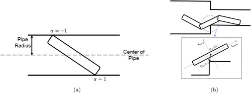
The conditions for determining contact situation are shown in Figure 4. The normal force acts on contact joint i in the y direction of local frame is determined by the distance between joint i and the center of pipe with same x coordinate. When the distance exceeds the radius of pipe, it is assumed that the contact is established. The contact parameter ${\alpha }_i$ is equal to $-1$ when the joint touches the upper side and 1 when having contact with the down side. After a collision takes place, the collision force is computed using a mass-spring-damper system, (8) $\begin{array}{rl}& F_{N,i}={\alpha }_i|(-k_{\mathrm{msd}}(D_i-R_p)-d_{\mathrm{msd}}{v}_i)|\end{array}$(8) (9) $\begin{array}{rl}& \{\begin{array}{ll}{\alpha }_i=-1,& \mathrm{if}{D}_i=y_{\mathrm{joint},i}-C_p>0\\ {\alpha }_i=1,& \mathrm{if}{D}_i=y_{\mathrm{joint},i}-C_p<=0\end{array}\end{array}$(9) where $D_i$ is the difference between the y-component $y_{\mathrm{joint},i}$ of joint i in the global frame and y coordinate of the related pipe center $C_p$ aligned to x axis, $R_p$ represents the pipe radius. $k_{\mathrm{msd}}$ and $d_{\mathrm{msd}}$ are the spring and damping coefficients. $v_i$ is the related velocity of joint i in the y-axis of the global frame.

An instance of discontinuous diameter change in the pipe, as illustrated in (b) of Figure 4, can result in the link establishing contact between the robot and the corner. It is assumed that contact force operates on the CM of the associated link. In the y-coordinate of the local frame, the distance from the corner point to the CM of the link is computed using the vector from link i to the corner. (10) $\begin{array}{r}{\mathrm{Distance}}_i=[0,1]({\text{R}}_{{\text{L}}_{\text{i}}}^{\text{global}}{)}^T{a}_i\end{array}$(10) where $a_i\in {\mathbb{R}}^2$ represents the vector from link i to the closest corner in the global frame, it is then transformed into the local frame by the rotation matrix and the y-component of this vector is extracted. In this research, the thickness of the link is not considered so the link i is assumed to have contact with the corner if the absolute value of ${\mathrm{Distance}}_i$ is smaller than 0.01 m.

Figure 4. Method of determine the contact direction of the related link body. (a) Contact happened at each joint (b) Contact occurs on the body of the link.

The friction force along the x-axis in the local frame between snake body and the pipe is incorporated into the system dynamics when the link makes contact with the pipe. It is demonstrated in [14] that the snake robot utilizes friction force to maintain its stability and resist the weight of the robot, which is supported by wall friction. Furthermore, the research demonstrates that the friction coefficient's value significantly influences the snake robot's locomotion. In the aquatic environment, the snake could propel itself forward using the friction force against the ocean current. Sliding friction in the tangential direction of local frame is computed as: (11) $\begin{array}{r}{f}_i=-{\mu }_f\mathrm{sgn}(v_{t,i})\left|\begin{array}{c}{F}_{N,i}\end{array}\right|\end{array}$(11) where ${\mu }_f$ is the friction coefficient, respectively. $v_{t,i}$ represents the tangential velocity in the local x coordinates.

3. Control method

In this section, the proposed control method will be introduced. First, four main stages of the Monte Carlo Model Predictive Control are presented. Once the new control input for the head joint has been generated, the joint angle is transmitted along the snake body using the Curvature Derivative Control. This work employs GPU parallel computing as opposed to CPU parallel computing, the distinction and benefit are also discussed in this section.

In [19,20], the Economic MPC is used for the control of the snake robot. This type of gradient-based MPC utilizes the gradient information of cost function to solve the optimization problem. MCMPC is a sample-based MPC that calculates the optimal input through random sampling, eliminating the requirement for gradient information. This provides the benefit that MCMPC can manage discontinuous situations in the prediction step through forward simulation, whereas gradient-based MPC faces challenges in this regard when employing backward simulation.

3.1. Monte carlo model predictive control

The procedure of MCMPC is proposed in detail in [23]. This kind of sample-based MPC takes the advantage of GPU parallel computing and is able to deal with huge amounts of threads in the same time. MCMPC is employed to manage contacts for various types of robotics, including collisions for the inverted pendulum swing up control on a cart in [24]. MCMPC is also used to control the quadcopter while considering collision with wall [25] and the trajectory generation of CM for Biped Robot taking contact with walls and constraints of ZMP into account [26].

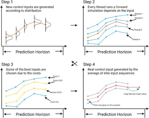
Figure 5 shows the four main procedures of MCMPC as:

1. At the outset of each control cycle, Monte Carlo random sampling is utilized to generate the control input sequences based on weighted mean(orange line) of previous step.

2. Every individual thread(blue lines) in the parallel computing framework executes a forward simulation of the dynamic system utilizing the control inputs that were produced in the preceding phase.

3. Following the calculation of the cost value of each thread, the elite samples(yellow lines) are selected according to the cost.

4. Depending on the input sequences of these elite samples(grey lines), the weighted mean(red line) is utilized for the next control loop.

The input sequence generated at each control loop is represented as $u_k^n=\{u_{k|1}^n,u_{k|2}^n,\dots ,u_{k|i}^n,\dots ,u_{k|N}^n\}$, where N is prediction horizon, n represents the index of threads, k is the number of control cycle of MCMPC which means the time, and i is the prediction step. The normal distribution $\mathcal{N}$ of Monte Carlo sampling is generated with weighted mean $u_{k-1}^{\ast }$ and standard deviation ${\sigma }_{k-1}$ as, (12) $\begin{array}{r}{u}_{\{k|i\}}^n\sim \mathcal{N}(u_{\{k-1|i+1\}}^{\ast },{\sigma }_{k-1}^2)\end{array}$(12) In this study, the value of standard deviation is held constant. However, it may be subject to variation if the increase of dynamic uncertainty is taken into account. Following the generation of the specified number of input sequences, forward simulation of each sequence is executed concurrently on each thread of GPU. The simulation is based on the state equation of the controlled system as, (13) $\begin{array}{r}{x}_{\{k|i\}}^n=f(x_{\{k|i-1\}}^n,u_{\{k|i\}}^n)\end{array}$(13) where x is the state variables. The designed cost function is then calculated using these state variables in order to determine which elites have the lowest cost value. Once all forward simulations have been completed, the elite samples are selected according to a certain rate. These samples are then utilized in the computation of the weighted average of the actual input sequence. (14) $\begin{array}{r}{u}_{\{k|i\}}^{\ast }=\frac{\sum _{q=1}^{Q_t}{u}_{\{k|i\}}^q{e}^{-\frac{L_k^q}{\lambda }}}{\sum _{q=1}^{Q_t}{e}^{-\frac{L_k^q}{\lambda }}}\end{array}$(14) where $L_k^q$ represents value of the cost function of q-th thread among elite threads during k-th control cycle, $Q_t$ is the number of chosen threads, q is the q-th thread among elite threads and λ is constant parameter, if $\lambda \to 0$, estimated optimal input matches real optimal input based on Pincus theorem [27]. The first step of optimal input sequence is applied to the real system. Therefore, optimal control laws for the prediction of next control cycle are described as, (15) $\begin{array}{r}{u}_{\{k|2\}}^{\ast },u_{\{k|3\}}^{\ast },\dots ,u_{\{k|N\}}^{\ast },u_{\{k|N\}}^{\ast }\end{array}$(15) The N+1 mean value for the prediction of next cycle is not estimated and it is expected that control inputs are usually continuous. Thus, it is simply coped as the same value as the Nth optimal control law.

Figure 5. The main procedures of MCMPC: Random input sequences are generated based on the weighted mean(the orange line) from previous step; Every thread(blue lines) runs a forward simulation based on the input sequences; Elite samples are chosen depend on the cost value(yellow lines are threads with small costs while blue ones are threads with high costs); The weighted mean(red line) is then calculated based on the elite threads(grey lines).

For MCMPC, constraints are established for both state variables and control inputs. For the head joint, the random inputs generated by MCMPC will be evaluated and set within a specified range to satisfy the input constraint. This constraint is straightforward to establish, as the generated value will be replaced with the constraint value when it surpasses the up and down limitations. In the event that the state deviates significantly from the specified limits of MCMPC, a substantial value will be appended to the cost. This augmentation serves the purpose of excluding threads that surpass the limit from the elite sample selection process.

For previous study [21], the parallel computation was devised in MATLAB. PARFOR function, which utilizes an eight-core CPU to execute programme calculations, was implemented. As previously stated, this methodology would result in an extended computation duration in comparison to gradient-based MPC. Research focusing on gradient-based MPC indicates that real-time implementation is not yet feasible due to its long computation time. Instead of MATLAB, CUDA is utilized in this work. The evidence demonstrates in the results section will show the contributions on the reduce of computation time.

3.2. Curvature derivative control

Following the generation of the head joint input by MCMPC, the other joints are controlled using Curvature Derivative Control (CDC). CDC is a type of control method that determines the ideal moment of bending while taking into account energy consumption of the associated joint torques. This method is proposed and utilized for the locomotion of snake robot in [28,29]. The joint torque is calculated according to the following equation: (16) $\begin{array}{r}{\tau }^{\ast }(s)=-\frac{\mathrm{m\alpha }}{{\int }_0^{L_{\mathrm{cdc}}}⟨{\kappa }^{\prime }(s),{\kappa }^{\prime }(s)⟩\mathrm{d}s}{\kappa }^{\prime }(s)\end{array}$(16) where ${\kappa }^{\prime }(s)\in \mathbb{R}$ signifies the curvatures with arclength s, ${\tau }^{\ast }(s)$ represents the bending moment distribution, α denotes the longitudinal acceleration, and $L_{\mathrm{cdc}}$ is the length of body curve. Following this, the articulated model is derived from the continuum model, with the joint torque replacing the bending moment and the curvature being substituted with the joint angle. The calculation of control inputs for joints, excluding the head joint, is as follows: (17) $\begin{array}{r}{\tau }_i=k_c({\varphi }_{i+1}-{\varphi }_i)-k_{\mathrm{cd}}{\dot{\varphi }}_i\end{array}$(17) where $k_c$ and $k_{\mathrm{cd}}$ are control gains with given constant values, ${\varphi }_i$ and $\dot{{\varphi }_i}$ represent the related joint angle and the joint velocity.

By employing this control method, the external environment's effect on one link can be transferred to the adjacent link, thereby adapting the snake's body to the varied surroundings. In addition to merely transmitting the joint angle to subsequent joints, propulsion forces that operate on preceding components can also be transferred to the succeeding link. It is important to note, however, that this method of control operates under the assumption that the snake robot body does not experience any side slip. Such conditions can be maintained for an underwater environment. In [29], Figure 10 in the paper illustrates the relationship between epaxial muscle activity and curvature, as observed in the behaviors of an actual snake.

Furthermore, it is demonstrated that advanced locomotion can be generated using CDC even in the absence of knowledge regarding the wall's geometry. This implies that snake robot consistently selects the most advantageous portion of contact area to facilitate its forward motion. This phenomenon is also observed when the robot is in motion within a restricted environment.

4. Simulation setup and related results

In this section, setups of the simulation environment are introduced also with parameters for MCMPC. Simulation results are shown under different initial conditions and analyzed at the end of this section. The control method is implemented in the CUDA v12.0. All the experiments are tested on the laptop with 11th Gen Intel(R) Core(TM) i7-11800H CPU and NVIDIA GeForce RTX 3060 Laptop GPU.

4.1. Simulation environment

The top $1\mathrm{\%}$ of random inputs are chosen as the elite threads. The prediction horizon is set to N=100 with a sampling time of $T_s=0.1$ s. Constraints of MCMPC for control input and individual joint angles are denoted as $|{\varphi }_i|\le 1.04$. Constraint for CDC is $|u_i|\le 0.5$ with $K_c=0.5$ and $K_{\mathrm{cd}}=1.5$, respectively. The snake robot consists of 10 links with total link length $l_{\mathrm{all}}=1.4$ m, total mass $m_{\mathrm{all}}=1$ kg, and Parameters for hydrodynamics are set as $\rho =1000$ $\mathrm{kg}/{\mathrm{m}}^3$, $C_M=0.5$, $C_f=0.03$, $C_A=1$ and $C_D=2$. Current values are established in accordance with the experimental conditions. The parameters of the MCMPC, CDC, and the initial conditions of CUDA are shown in Table 2.

Table 2. Parameters for MCMPC.

Name	Meaning	Value
Prediction Horizon	Time interval of the prediction of MCMPC	10s
Prediction Steps	Number of predictions for one horizon	100
Number of Samples	Total samples for random sampling of MCMPC	8640
Number of Iterations	Times of repetition for each control loop	1
${\sigma }^2$	Variance of normal distribution for input sequence	0.1
Input Constraints	Constraints for inputs generated by MCMPC	$-1.04<u_i<1.04$

The cost function includes a position error of the CM and the destination with control inputs is given by (18) $\begin{array}{rl}{L}^n& =\sum _{i=1}^N{x}_{\{k|i\}}^{T}Q{x}_{\{k|i\}}+u_{\{k|i\}}^{T}R{u}_{\{k|i\}}\end{array}$(18) (19) $\begin{array}{rl}{x}_{\{k|i\}}& =\left[\begin{array}{c}{p}_x\\ p_y\end{array}\right]-\left[\begin{array}{c}{D}_x\\ D_y\end{array}\right]\end{array}$(19) where $D_x,D_y$ are the coordinates of the final destination, $Q=\left[\begin{array}{cc}10& 0\\ 0& 50\end{array}\right]$ and R=0.5. The values of Q are chosen for the performance of snake robot. y component is greater than x component in this study, as it is presumed that the robot will initially dive priorly in y direction and then proceed towards the entrance of along x direction. This provides the robot with additional space to adjust the proper angle of entry (large weight converges faster).

4.2. Simulation results

In this study, various pipe configurations are examined in order to validate the capability of the proposed control method to accommodate pipes with varying diameters and structures. The robot will identify the pipe as the entrance to access the interior and reach the destination. The initial position of the head joint of the robot is (0,0) with zero initial states.

The vertical alignment of the wall serving as the exterior surface of the sunken ship is established at an x-coordinate of -5. The entrance locations remain consistent across all experiments. The time progression is indicated by the varying shades of the lines in each of the resultant representations in Figures 6–9, 11. This suggests that the initial condition of the robot at the start of the experiment is denoted by light-colored lines, while the state after a specific length has passed is represented by dark-colored lines, respectively.

Figure 6. Results of snake robot moving through a pipe with continuous change of the diameter. (a) Pipe with decreasing diameter (b) Pipe with increasing diameter.

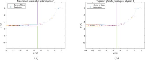
Figure 7. Results of snake robot moving through a pipe with discontinuous change of the diameter. (a) Pipe with decreasing diameter (b) Pipe with increasing diameter.

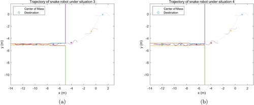
Figure 8. Results of snake robot moving through a pipe with a bend. (a) Pipe with a turn structure.

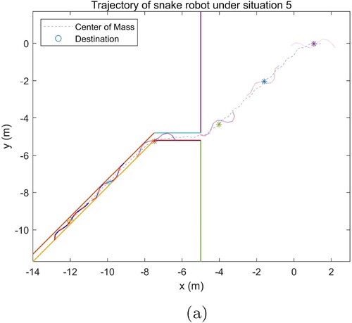
Figure 9. Results of snake robot moving through a pipe with MCMPC and with a given joint reference both in 60 s (a) Locomotion with MCMPC for the head joint (b) Locomotion with given reference for the head joint.

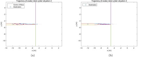
Figure 10. Success rate of entering the pipe for MCMPC with and without the contact dynamic during prediction steps. (a) The number of samples for generating the random input sequences of MCMPC.

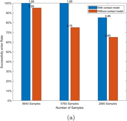
Figure 11. Results of MCMPC with and without contact model during prediction steps under situation 5 both in 90 s (a) Locomotion with contact model (b) Locomotion without contact model.

4.3. Continuously change of pipe diameter

As a simulation scenario, a pipe with a continuously changing radius is initially evaluated. The pipe initially holds a radius of 0.2 m. However, after deviating by -7.5 m, its diameter gradually reduces to 0.1 m and keeps constant after x=−10. In the second experiment, which is designed to examine the inverse circumstance, the pipe's radius begins at 0.1 m and gradually increases to 0.2 m. The simulation configurations for both investigations are identical.

The results in Figure 6 are illustrated. The snake-like robot, as depicted in the figure, advances from its initial position toward the entrance. Without a given reference, MCMPC and CDC generate the snake robot's locomotion pattern at random, and the robot is capable of adjusting the amplitude of the moving wave as it traverses different environments. Once the robot reaches the entrance of the pipe, it proceeds inside and executes a travelling wave locomotion resembling a trapezium, as a result of its physical constraints. Assuming that the ocean current occurs only along the global x-axis within the pipe, its velocity is held constant at 0.1 m/sec for the shorter sections and 0.2 m/sec for the larger sections. In addition, the results demonstrate that the snake robot is adaptable to both scenarios, as its locomotion amplitude would vary in accordance with the pipe's diameter.

4.4. Discontinuous change of pipe diameter

The pipe's discontinuous section is subsequently examined by the snake robot. The initial conditions for the robot are identical to those of the preceding tests. In the first simulation of this section, the pipe's diameter is initialized at 0.4 m between coordinates x=−5 and x=−7,5. It then stabilizes at 0.2 m thereafter. The pipe's center is located at y=−5. The second simulation examines the opposite scenario. The ocean current is maintained at the same velocity of 0.1 m/sec for thinner pipe segments and 0.2 m/sec for the remaining pipe segments. The link body and the stage may come into contact due to the discontinuous connection between the two sections of the pipes. As previously stated, the system dynamics takes into account this type of contact situation, and the associated contact force exerts an influence on the link's center of mass.

Figure 7 shows the related results. The initial conditions for both simulations are identical. In both scenarios, the robot executes smooth locomotion in order to approach the tunnel's entrance. Throughout operation, the robot's locomotion varies in response to the physical limitations of its surroundings, demonstrating its adaptability to different environments. Even after reaching the final destination, the robot continues to generate slowly movements in order to maintain stable in the face of current influence.

4.5. Pipe with a bend structure

Another situation of the pipe is that it is bent at the point where it meets the horizontal section. Figure 8 shows the simulation result. The pipe is characterized by a flat part with a diameter of 0.4 m, a turn occurring at the point where x=−7.5, and a degree of ${45}^{\circ }$. Likewise, the diameter is altered to 0.28 m, respectively. The ocean current exerts an influence on the y-axis of the inclined parts, causing a change of 0.1 m/sec in both the x and y coordinates. The result shows that the snake robot successfully enters the pipe. When it comes to the bending part, the locomotion of the robot also changes to pass through the bend.

Additionally, the result indicates that the snake robot generates propulsion force by pressing its body against the blue portion of the pipe, thereby enabling it to move forward in the same direction as the pipe. This type of propulsion facilitated by contact exhibits the same characteristics as obstacle-assisted locomotion.

It is worth noting that the snake robot, with the assistance of the CDC, would select the essential parts from each side of the pipe in order to produce advanced locomotion in each of these scenarios. An instance of this characteristic is also noted in the study [29], where the CDC is applied to regulate a snake robot within a constricted, twisting environment.

4.6. Efficiency of MCMPC

This section provides an analysis of the benefits associated with employing MCMPC for the head joint. To demonstrate the efficacy of MCMPC, the head joint of the snake robot is referenced with a sinusoidal input for comparison. The remaining joints are controlled by CDC in the same manner as the proposed method. Pipes with continually varying diameters are tested.

The robot is configured to begin its trajectory at the entry of the pipe. Both experiments simulate the performance of 60-second results. The following specifies the input reference for the head joint: (20) $\begin{array}{r}{u}_{\mathrm{ref}}=1.04\sin (2.2t_{\mathrm{ref}})\end{array}$(20) where $t_{\mathrm{ref}}$ represents the simulation time. The frequency and the amplitude are set the same as for the MCMPC.

Figure 9 illustrates results of the associated experiment. Both snake robots demonstrate the capacity to advance in response to a pipe diameter change. Due to the fixed reference, the snake robot was unable to change its locomotion in case (b). This results in increased extra contact with the pipe, thereby impeding the velocity of motion. In contrast, the snake robot shown in (a) is more adaptable across environments and can therefore travel further in the same amount of time due to the assistance of MCMPC.

For comparisons of both control methods, the efficiency of MCMPC is demonstrated above. However, comparing results of ‘with and without CDC’ is difficult. It is challenging to set up each joint as control input for MCMPC. Because the computation becomes more complicated as the quantity of inputs increases and amplifies with the complexity of dimensions. Consequently, CDC is utilized for all simulations.

4.7. Benefits of contact model

This section demonstrates the impact of incorporating the contact model into the MCMPC prediction stages. In the prediction stages, two MCMPC prediction models are evaluated both with and without the contact dynamic. Failure to incorporate the contact dynamic into the prediction stages of MCMPC would result in the robot failing to anticipate a collision prior to its occurrence. The robot starts from the initial position of (0,0) in order for it to move in proximity to the destination. The entrance portion of the pipe is configured with a diameter of 0.2 m, which is marginally inadequate for the snake robot to traverse. The investigations are simulated using three different sample amounts for MCMPC: 8640, 5760, and 2880, with each scenario being executed 20 times.

Figure 10 illustrates experimental results associated with the given variable.

An increased quantity of samples results in enhanced efficacy of the robot, enabling it to enter the pipe. The circumstance in which the robot is unable to enter is due to a trajectory change caused by the head of the robot colliding with the wall. Based on the results of the experiment, MCMPC with contact model successfully entered the tube for both 8640 and 5760 samples. However, the possibility of without contact model decreased from 0.95 to 0.75, suggesting that the robot's failure probability may be higher in the absence of contact model. With a reduced number of samples (2880), both models experience a failure condition due to the diminished likelihood of diverse gait patterns. Performance is invariably enhanced when contact model is incorporated into MCMPC prediction stages. It is noteworthy to remark that the computation time for MCMPC remains almost the same whether the contact model is utilized or not.

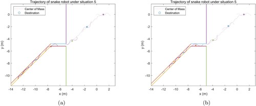
Figure 11 shows experiment results of two situations with 8640 samples. All of the snake robots manage to traverse the pipe's entrance successfully. However, collisions occur once the robots enter the pipe, and it is observed that the model of the robot without contact makes needless contact with the pipe. Without contact information detected during the prediction phase of MCMPC, the head link of the robot would collide with the pipe. Consequently, the contact model-equipped robot arrives at the designated location within 90 s of simulation time, whereas another robot is still en route to the same destination. The robot without contact model depicted in (b) continues to advance along the pipe's narrow structure with the assistance of the CDC and reaches its destination in 120 s.

4.8. Computational cost

In previous research [20,21], the computational time for either MCMPC in MATLAB or Economic MPC required a substantial amount of time to calculate. As mentioned in [20], the computation of individual optimal inputs in the simulations requires a time interval of 5 to 200 s. The desktop computer executes the simulation using C code generated on a virtual machine. The main difference between the dynamic model of the snake robot and the one investigated in this work is that the former operates on land, whereas the latter operates underwater. Additionally, it is noted that no attempt is made to decrease the computation time in [20]. In our previous work [21] realizing MCMPC and CDC for the obstacle-aided locomotion for the underwater snake robot. The computation of a single input sequence requires between 30 and 60 s and is performed in MATLAB 2021b utilizing CPU parallel computing. The program operates on the identical laptop as this study.

GPU parallel computing is accomplished with CUDA, the calculation time for each control cycle of each input sequence is displayed in Table 3. The calculation time is significantly impacted by the number of samples, as it determines the complexity of MCMPC. By utilizing GPU parallel computation, each control input sequence is generated within the control cycle of 0.1 s. The time required decreases as the number of threads decreases. However, it is evident from the results that as the number of samples increases, so does the success rate of obtaining complete performance for the locomotion of the snake robot. The 2880-thread based snake robot might be unable to reach the intended location.

Table 3. Computation time for each control method.

Control Method	Time consumed for each optimal input
Economic MPC	between 5 and 200 s
MCMPC(CPU parallel computing)	between 30 and 60 s (4000 threads)
MCMPC(GPU parallel computing)
8640 Threads	Average 0.098 s
5760 Threads	Average 0.056 s
2880 Threads	Average 0.033 s

5. Conclusions and future works

The present study introduced sample-based Monte Carlo Model Predictive Control and Curvature Derivative Control as control strategies for a two-dimensional underwater snake robot. By utilizing MCMPC and CDC, the snake robot achieves more efficient locomotion in response to different kinds of environment result in a better performance than a given fixed reference. Through the implementation of GPU parallel computing, the time for the Monte Carlo random sampling procedure is drastically decreased compared to previous methods.

Simulation results show that by incorporating contact dynamics into the MCMPC prediction stages, the robot is capable of successfully passing the pipe through the entrance while the robot is located external to the wall initially. The snake robot is designed to exhibit adaptive mobility in order to navigate through diverse settings, such as varied pipe constructions with varying geometric constraints, and successfully reach its desired goal. The robot also possesses the capability to maintain stability in the presence of a current.

Nevertheless, proposed control approach fails to perform concertina locomotion in confined spaces. Because rest of snake's body merely amplifies the motion produced by the head. In [30], Tegotae-based control was utilized with CDC to generate autonomous gait pattern that achieved both concertina locomotion and scaffold-based locomotion. This kind of advantage will be considered to improve the performance in the future. Future works will also entail separate control of snake body components to achieve numerous objectives. As an example, MCMPC generates control inputs at the head and middle joint, allowing one part of the body to grasp the object while the other part propels the robot forward. Furthermore, design and implementation of the proposed method to an actual snake robot are future plans.

Disclosure statement

No potential conflict of interest was reported by the author(s).

Additional information

Funding

This work was supported by JSPS KAKENHI [grant number 23K03896].

Notes on contributors

Yiping Qiu

Yiping Qiu received the B.E. from Yangzhou University in 2018. He received the MSc Advanced Control and Systems Engineering from The University of Manchester, in 2019. He is currently a Ph.D. candidate in the Graduate School of Science and Technology, University of Tsukuba. His research interests include the Model predictive control for underwater snake robot.

Hisashi Date

Hisashi Date received the M.E. and Ph.D. degrees from Tokyo Institute of Technology in 2000 and 2003, respectively. From 2003 to 2013, he was Research Associate in the Department of Computer Science, National Defense Academy. From 2013 to 2015, he was Lecturer in the same department. From 2005 to 2006, he was a visiting associate at the Department of Mechanical Engineering, California Institute of Technology. Since 2015, he has been Associate Professor at the Institute of Systems and Information Engineering, University of Tsukuba. His current research interests are in nonlinear model predictive control and autonomous robots.

References

- Hirose S. Snake-like locomotors and manipulators. Biologically Inspired Robots. 1993.
- Kelasidi E, Pettersen KY, Gravdahl JT, et al. Modeling of underwater snake robots. In: 2014 IEEE International Conference on Robotics and Automation (ICRA); IEEE; 2014. p. 4540–4547.
- Boyer F, Porez M, Khalil W. Macro-continuous computed torque algorithm for a three-dimensional eel-like robot. IEEE Trans Robot. 2006;22(4):763–775. doi: 10.1109/TRO.2006.875492
- Khalil W, Gallot G, Boyer F. Dynamic modeling and simulation of a 3-d serial EEL-like robot. IEEE Trans Syst, Man, Cyber, Part C (Appl Rev). 2007;37(6):1259–1268. doi: 10.1109/TSMCC.2007.905831
- Liljebäck P, Pettersen KY, Stavdahl Ø, et al. Snake robots: modelling, mechatronics, and control. London: Springer; 2013.
- Pettersen KY. Snake robots. Annu Rev Control. 2017;44:19–44. doi: 10.1016/j.arcontrol.2017.09.006
- Liu J, Tong Y, Liu J. Review of snake robots in constrained environments. Rob Auton Syst. 2021;141:103785. doi: 10.1016/j.robot.2021.103785
- Liljeback P, Pettersen KY, Stavdahl Ø, et al. Hybrid modelling and control of obstacle-aided snake robot locomotion. IEEE Trans Robot. 2010;26(5):781–799. doi: 10.1109/TRO.2010.2056211
- Kelasidi E, Pettersen KY, Gravdahl JT, et al. Modeling and propulsion methods of underwater snake robots. In: 2017 IEEE Conference on Control Technology and Applications (CCTA); IEEE; 2017. p. 819–826.
- Kano T, Ishiguro A. Obstacles are beneficial to me! Scaffold-based locomotion of a snake-like robot using decentralized control. In: 2013 IEEE/RSJ International Conference on Intelligent Robots and Systems; IEEE; 2013. p. 3273–3278.
- Inazawa M, Takemori T, Tanaka M, et al. Motion design for a snake robot negotiating complicated pipe structures of a constant diameter. In: 2020 IEEE International Conference on Robotics and Automation (ICRA); IEEE; 2020. p. 8073–8079.
- Hirose S, Umetani Y. Kinematic control of active cord mechanism with tactile sensors. Trans Soc Instru Control Eng. 1976;12(5):543–547. doi: 10.9746/sicetr1965.12.543
- Nakajima M, Tanaka M, Tanaka K, et al. Motion control of a snake robot moving between two non-parallel planes. Adv Robot. 2018;32(10):559–573. doi: 10.1080/01691864.2018.1458653
- Barazandeh F, Bahr B, Moradi A. How self-locking reduces actuators torque in climbing snake robots. In: 2007 IEEE/ASME international conference on advanced intelligent mechatronics; IEEE; 2007. p. 1–6.
- Shapiro A, Greenfield A, Choset H. Frictional compliance model development and experiments for snake robot climbing. In: Proceedings 2007 IEEE International Conference on Robotics and Automation; IEEE; 2007. p. 574–579.
- Kuwada A, Wakimoto S, Suzumori K, et al. Automatic pipe negotiation control for snake-like robot. In: 2008 IEEE/ASME International Conference on Advanced Intelligent Mechatronics; IEEE; 2008. p. 558–563.
- Virgala I, Kelemen M, Prada E, et al. A snake robot for locomotion in a pipe using trapezium-like travelling wave. Mech Mach Theory. 2021;158:104221. doi: 10.1016/j.mechmachtheory.2020.104221
- Kelasidi E, Liljeback P, Pettersen KY, et al. Innovation in underwater robots: biologically inspired swimming snake robots. IEEE Robot Automat Magaz. 2016;23(1):44–62. doi: 10.1109/MRA.2015.2506121
- Nonhoff M, Köhler PN, Kohl AM, et al. Economic model predictive control for snake robot locomotion. In: 2019 IEEE 58th Conference on Decision and Control (CDC); IEEE; 2019. p. 8329–8334.
- Müller E, Köhler PN, Pettersen KY, et al. Economic model predictive control for obstacle-aided snake robot locomotion. IFAC-PapersOnLine. 2020;53(2):9702–9708. doi: 10.1016/j.ifacol.2020.12.2622
- Qiu Y, Date H. Obstacle-aided locomotion for underwater snake robot using monte carlo model predictive control and curvature derivative control. In: 2023 62nd Annual Conference of the Society of Instrument and Control Engineers (SICE); IEEE; 2023. p. 690–695.
- Jordan CE. Coupling internal and external mechanics to predict swimming behavior: a general approach. Am Zool. 1996;36(6):710–722. doi: 10.1093/icb/36.6.710
- Ohyama S, Date H. Parallelized nonlinear model predictive control on gpu. In: 2017 11th Asian Control Conference (ASCC); IEEE; 2017. p. 1620–1625.
- Nakatani S, Date H. Swing up control of inverted pendulum on a cart with collision by monte carlo model predictive control. In: 2019 58th Annual Conference of the Society of Instrument and Control Engineers of Japan (SICE); IEEE; 2019. p. 1050–1055.
- Kato M, Date H, Nakatani S, et al. Control of quadcopter considering collision with wall utilizing monte carlo model predictive control. Trans Soc Instrum Control Eng. 2021;57(9):379–390. doi: 10.9746/sicetr.57.379
- Ando H, Nakatani S, Date H. Trajectory generation of center of mass for biped robot by monte carlo model predictive control considering upper body contact with walls and constraints of zmp. Trans Soc Instru Control Eng. 2023;59(3):162–175. doi: 10.9746/sicetr.59.162
- Pincus M. -A closed form solution of certain programming problems. Oper Res. 1968;16(3):690–694. doi: 10.1287/opre.16.3.690
- Date H, Takita Y. Control of 3d snake-like locomotive mechanism based on continuum modeling. In: International Design Engineering Technical Conferences and Computers and Information in Engineering Conference; Vol. 47438; 2005. p. 1351–1359.
- Date H, Takita Y. Adaptive locomotion of a snake like robot based on curvature derivatives. In: 2007 IEEE/RSJ International Conference on Intelligent Robots and Systems; IEEE; 2007. p. 3554–3559.
- Kano T, Yoshizawa R, Ishiguro A. Tegotae-based decentralised control scheme for autonomous Gait transition of snake-like robots. Bioinspir Biomim. 2017;12(4):046009. doi: 10.1088/1748-3190/aa7725